1. Introduction
With the rapid development of computer vision technology, multi-view stereo (MVS) has become a highly prominent field of interest. Research in MVS aims to reconstruct three-dimensional information of a scene from multiple perspective images with known camera parameters, playing a crucial role in various domains such as virtual reality, augmented reality, and visual effects in the film industry.
In existing MVS methods, traditional methods based on geometric context [
1,
2,
3,
4,
5] have achieved good reconstruction results in texture-rich areas, especially in terms of accuracy. However, challenges persist in reconstructing the three-dimensional information of the scene from images in areas with low texture, image occlusions, variations in radiance, or non-Lambertian surfaces. To address this issue, some researchers [
6] have employed deep learning techniques, utilizing Convolutional Neural Network (CNN) to extract image features. They perform robust feature matching within the field of view of the reference camera to construct a cost volume representing the geometric information of the scene. Subsequently, they employ a 3D U-Net network for regularization to regress depth maps. Finally, the scene’s three-dimensional information is reconstructed through depth maps fusion. While this approach enhances the overall quality of reconstructing scenes, it encounters challenges in challenging areas with low texture or non-Lambertian surfaces, where features at the same 3D position exhibit significant differences between different views. Incorrect feature matching results in the construction of the flawed cost volume by the network, leading to poor completeness in the final reconstruction. This is due to traditional CNN having fixed receptive field sizes, which limit feature extraction networks to capture only local features, hindering the perception of global contextual information. The lack of global contextual information often causes the network to exhibit local ambiguities in challenging regions, thus reducing matching robustness. Recent studies have employed self-attention mechanism [
7,
8] to capture crucial information for cost volume computation by considering context similarity and spatial proximity. This has improved matching robustness and enhanced the ability of the cost volume to represent scene geometry information. However, there remains significant potential for enhancing the reconstruction quality, especially in challenging areas.
Recently, the Neural Radiance Field (NeRF) [
9] rendering technique has made significant advancements in the fields of computer vision and computer graphics. NeRF models view-dependent photometric effects using differentiable volume rendering, enabling it to reconstruct implicit 3D geometric scenes. Additionally, it learns volume density, which can be interpreted as depth, allowing it to explicitly represent the reconstructed geometric scene information through indirectly rendering depth. Subsequent works [
10,
11,
12,
13,
14,
15] have focused on accelerating its rendering speed and implicitly learning the 3D scene’s geometry with a strong generalization capability by inputting a few views and combining them with the MVS network to synthesize higher-quality novel views or more accurate depth maps. However, these efforts have primarily advanced the development of the Neural Radiance Field while overlooking the quality of point cloud reconstruction by the MVS network. Therefore, our method leverages the precise neural volume rendering of the Neural Radiance Field to build 3D geometric information about the scene. This approach enables the rendering of depth, even in challenging areas with low texture or non-Lambertian surfaces, allowing the MVS network to learn rich scene geometry information beyond the cost volume that represents scene geometry. This overcomes issues arising from rough depth maps due to incorrect matching in the network, ultimately enhancing the quality of the reconstructed point cloud.
In conclusion, we propose an end-to-end MVS network based on attention mechanism and neural volume rendering. By combining dilated convolution and attention mechanism during feature extraction, we extract rich feature information. This allows the network to achieve reliable feature matching in challenging regions. Leveraging the capacity of neural volume rendering to resolve scene geometry information, our approach mitigates the impact of the flawed cost volume arising from incorrect feature matching. Our method exhibits high completeness in reconstructing point clouds on the competitive DTU dataset concerning indoor objects and demonstrates robust performance on the Tanks and Temples dataset, which pertains to outdoor scenes. It outperforms many learning-based MVS networks, thus advancing 3D reconstruction based on MVS networks in crucial domains such as virtual reality, augmented reality, autonomous driving, and other significant applications.
In summary, our primary contributions can be outlined as follows:
We introduce a multi-scale feature extraction module based on triple dilated convolution and attention mechanism. This module increases the receptive field without adding model parameters, capturing dependencies between features to acquire global context information and enhance the representation of features in challenging regions;
We establish a neural volume rendering network using multi-view semantic features and neural encoding volume. The network is iteratively optimized through the rendering reference view loss, enabling the precise decoding of the geometric appearance information represented by the radiance field. We introduce the depth consistency loss to maintain geometric consistency between the MVS network and the neural volume rendering network, mitigating the impact of the flawed cost volume;
Our approach demonstrates state-of-the-art results on the DTU dataset and the Tanks and Temples dataset.
The remaining structure of this paper is as follows. In
Section 2, we present an overview of related work related to learning-based MVS networks and neural volume rendering. Subsequently, in
Section 3, we delve into the various components of our proposed MVS network based on attention mechanism and neural volume rendering.
Section 4 reports an extensive set of experimental results on the DTU dataset and the Tanks and Temples dataset, supplemented by ablation experiments to validate the effectiveness of the proposed modules. Finally, in
Section 5, we offer the conclusion of the article.
3. Methods
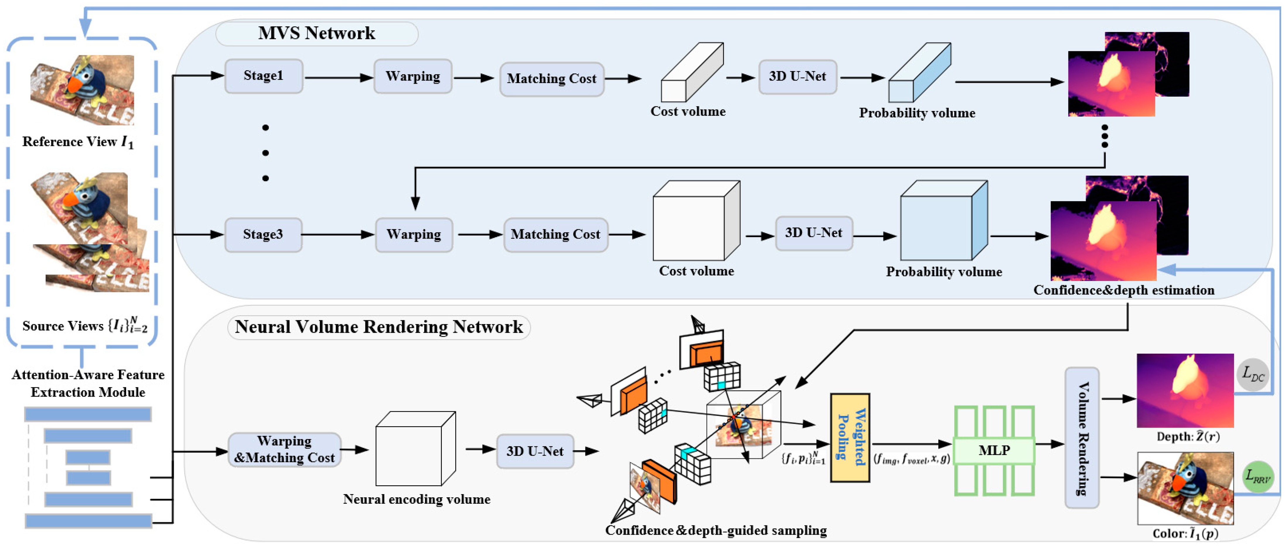
In this section, we elucidate the overall architecture of the proposed method, as illustrated in
Figure 1. This architecture primarily comprises the MVS network and the neural volume rendering network. Specifically, in the feature extraction stage, we introduce the attention-aware feature extraction module. This module combines dilated convolution with attention mechanism to extract more comprehensive feature information. The MVS network progressively constructs a probability volume in a coarse-to-fine manner to estimate the depth maps and confidence maps. Subsequently, we design a novel neural volume rendering network.
The multi-layer perceptron (MLP) network uses multi-view 2D feature along with the 3D neural encoding volume containing geometric-aware information as the mapping condition. Additionally, we adopt a uniform sampling strategy guided by depth maps and confidence maps to focus the scene sampling on the estimated depth surface region. Finally, we apply the rendering reference view loss to precisely resolve the geometric shape of the scene from the radiance field. We also introduce the depth consistency loss to ensure geometric consistency between the MVS network and the neural volume rendering network. It is noteworthy that the proposed network architecture functions as a universal framework for training the MVS network, making it applicable to any learning-based MVS network. The two networks provide mutual supervision and are simultaneously optimized.
3.1. Attention-Aware Feature Extraction Module
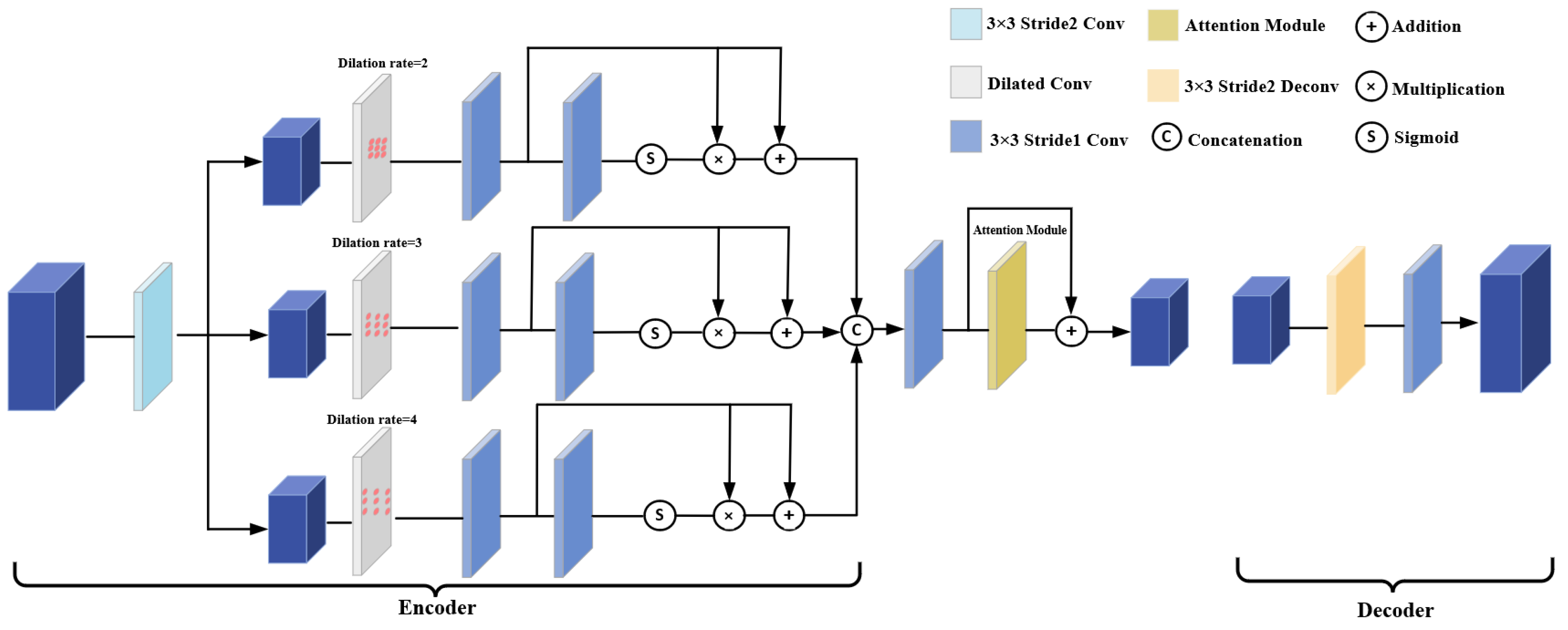
We propose the attention-aware feature extraction module. This module exhibits resemblances to a 2D U-Net, featuring elementary units that encompass both an encoder and a decoder, complete with skip connections. The encoder forms a network composed of dilated convolutional layers and an attention module, as depicted in
Figure 2. In the encoder section, the features are initially subsampled using a convolutional layer with a stride of 2. Subsequently, dilated convolutional layers with 3 × 3 kernel are employed to expand the receptive field of the input features. To address potential information correlation issues associated with the use of dilated convolution, we adopt a strategy similar to that of [
23], where feature maps are passed through a residual network structure with Sigmoid function after undergoing dilated convolutional layer with different dilation rate. To create the final feature map, the three fine-grained features are combined and run through a convolutional layer with an attention module. A convolutional layer and deconvolutional layer with 3 × 3 kernel make up the decoder. When provided with a reference image
and source images
at a resolution of
captured from different viewpoints, the attention-aware feature extraction module outputs three different scales of features, denoted as
, where
represents the
-th stage.
Figure 3 provides a visual representation of the attention module’s architectural design. The features, which have undergone triple dilated convolution, are input into two convolutional layers with 3 × 3 kernel. Each of these layers goes through Group Normalization (GN) and a ReLU activation function. Subsequently, we incorporate a LayerScale-based local attention layer [
24]. The operational details of this local attention layer are elucidated in
Figure 4, illustrating the mapping of queries and a collection of key-value pairs to generate an output, with pixel outputs computed via Softmax operation.
In this equation,
and
represent the queries, keys, and values, respectively, with the matrices
composed of learnable parameters. Here,
denotes a local region with a 3 × 3 input size. To address the issue of permutation equivariance resulting from the lack of encoded positional information, we introduce relative positional embeddings by incorporating learnable parameters into the keys, as described in [
25]. The relative distance vector
is partitioned along the dimensions, with half of the dimension of the output channel allocated for encoding the row direction and the remaining half for encoding the column direction. Furthermore, the features
, produced by the attention layer, need to be multiplied by the learned diagonal matrix weights within the network.
where
to
are learnable weights.
3.2. Cost Volume Construction
Subsequently, we perform adaptive depth hypothesis sampling using
layers of depth hypothesis planes
. Based on these assumptions, we construct feature volumes
, which are constructed by differential warping 2D source views features to the reference view. Under the depth plane hypothesis
, the warping between a pixel
in the reference view and its corresponding pixel
in the
-th source view is defined as follows:
where
and
are the intrinsic matrix of the
-th source camera and the reference camera, respectively,
and
represent the rotation and translation between the two views.
Subsequently, we consolidate multiple feature volumes
into a 3D cost volume
using the variance-based aggregation strategy. Then, the cost volume is then regularized into a depth probability volume using a 3D U-Net. We determine the probability
on a specified depth plane
for the pixel
in the reference view. Following this, we calculate the estimated depth value
for the pixel
using the method outlined below:
3.3. Neural Volume Rendering Network
To further alleviate the issue of incorrect feature matching in MVS caused by significant differences in 3D location of features between adjacent views, we introduced a neural volume rendering network. This network is trained in a self-supervised manner to learn the scene geometry, providing the network with rich scene geometry information. This addition helps mitigate the impact of the flawed cost volume generated by incorrect matching issues in the MVS network.
3.3.1. Scene Representation Based on Multi-View Features and Neural Encoding Volume
Our network extracts potential 2D feature vectors from the encoded contextual information of the source views. These multi-view 2D features provide additional semantic information about the scene, addressing 3D geometric ambiguity and enhancing the network’s ability to handle occlusion. Inspired by PixelNeRF [
13], we project 3D points from arbitrary space into the input multi-view images. For N different views
, each having its corresponding extrinsic matrix
concerning the target reference image and intrinsic matrix
. To acquire the color
and volume density
of the 3D point, we begin by converting its 3D position
, and its reference view direction
, into the coordinate system of each view, leading to the 3D point
. Subsequently, we project this point onto the corresponding pixel and feature maps and employ bilinear interpolation to sample its pixel
, and feature vector
:
where
represents the projection of the 3D point
’s reference view direction onto the respective observation directions of the multi-view images.
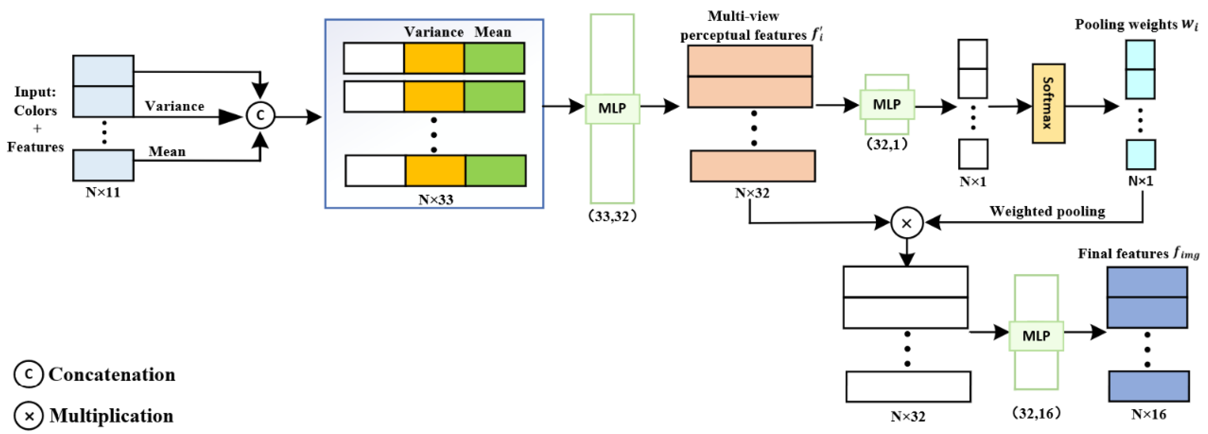
We utilize a weighted pooling operator, denoted as
, to aggregate the multi-view feature vectors, as illustrated in
Figure 5. Initially, we combine the feature vector
with the pixel information
to create a two-dimensional feature vector. Subsequently, we compute the mean
and variance
of the two-dimensional feature vector to capture both local and global information. Then, the two-dimensional feature vector is concatenated with
and
fed into our specially designed lightweight MLP, extracting the multi-view perceptual features, denoted as
, and the pooling weights, denoted as
. Finally, by applying a Softmax operation to the weight vector, we perform a weighted pooling operation on the multi-view perceptual features, resulting in the final feature vector
:
Subsequently, following the same approach as in RC-MVSNet [
22], we performed trilinear interpolation on the 3D neural encoding volume constructed using MVS, resulting in voxel-aligned three-dimensional feature voxel denoted as
. We then passed the weighted pooled final feature vector
and the three-dimensional feature voxel
through an MLP network to obtain RGB color
and volume density
at 3D sampling points in the reference view direction.
where, the position encoding function
aids in the network’s ability to recover high-frequency depth information.
3.3.2. Confidence and Depth-Guided Sampling for Volume Rendering
In the reference view
, each pixel
corresponds to a ray defined in the world coordinate system. The 3D point associated with the pixel
along this ray originating at a distance
from the origin
can be represented as
. To render the color
at the pixel
, rays are uniformly sampled at
discrete sample distances
within the original NeRF near and far planes
. The radiance field
at the 3D point is then queried:
Due to the uniform sampling probability within a sampling range in the original NeRF, the points may not be concentrated on the surface of the object, leading to a decrease in the quality of the rendered reference view. Therefore, for pixel , we propose to sample candidate points under the guidance of the prior range defined by the depth estimation value and its confidence from the MVS network.
We define the standard deviation
as the degree of confidence for pixel
with depth estimation value
:
The potential location of the object surface corresponding to each pixel should be confined within the interval defined by the depth estimation value
and the standard deviation
, represented as
:
Confidence and depth range
contain valuable signals to guide sampling along rays, thus, for rendering the color of a 3D point
in the geometric scene, we replaced the coarse network used for hierarchical sampling in the original NeRF. We distribute half of the sampled points between the near plane
and the far plane
. The second half of the sampled points are extracted within the range of the confidence and depth prior
. This ensures both the network’s generalization capability and model convergence.
Figure 6 presents a comparison between the two sampling methods.
Next, we render the predicted colors and volume density values
for each sampling point into the predicted reference pixel:
where
represents the cumulative transmittance along the ray
, and
is the distance between adjacent samples.
Our objective is to precisely deduce the depth value corresponding to the reference view from the radiance field. Therefore, we achieve the depth value for pixel
by performing a density integral along the rays in the direction of the reference view.
3.4. Loss Function
Within the neural volume rendering network, following the methodology established in the original NeRF, we introduce the rendering reference view loss. This loss function utilizes mean squared error to quantify the disparity between the color of volume rendering along rays from the reference view and the color of the corresponding ground truth reference view. By optimizing the pixel values of the rendered reference view
, we enhance the implicit geometric representation capability of the 3D scene.
To ensure geometric consistency between the two networks, we propose the depth consistency loss. This loss function employs
loss to minimize the difference between the rendered depth and the estimated depth from the MVS network, while also minimizing the difference between the rendered depth and the ground truth depth.
Within the MVS network, we utilize the
loss as the training loss, quantifying the divergence between the ground truth depth and the estimated depth.
In the end, the overall training loss function for the end-to-end network is given by the following:
4. Experiments
We comprehensively present the performance of our proposed method through a series of experiments. Additionally, we perform ablation experiments to validate the efficacy of our proposed attention-aware feature extraction module, loss functions, and the confidence and depth-guided sampling strategy.
4.1. Datasets
We conducted model training and evaluation using the DTU dataset [
26] and the Tanks and Temples dataset [
27]. The DTU dataset comprises 124 scenes captured from 49 distinct viewpoints, covering a range of 7 diverse lighting conditions, and collected using a robotic arm in indoor environments. We assess the reconstructed point cloud using three measurement criteria: Accuracy, Completeness, and Overall.
Accuracy represents the average distance between the reconstructed point cloud and the ground truth point cloud, calculated by the Formula (20). Completeness indicates the number of surfaces from the ground truth point cloud that are captured in the reconstructed point cloud within the same world coordinates, computed using Formula (22). Overall is the average of Accuracy and Completeness, calculated as per Formula (23).
where
denotes the reconstructed point cloud,
represents the ground truth point cloud, and
signifies the shortest distance from a point in the reconstructed point cloud to the ground truth point cloud.
where
represents the shortest distance from a point in the ground truth point cloud to the reconstructed point cloud.
The Tanks and Temples dataset, on the other hand, captures complicated real-world sceneries with 8 intermediate subsets and 6 advanced subsets.
We utilize the F-score as the evaluation metric for the Tanks and Temples dataset. The F-score takes into account the precision
and recall
of the reconstructed point cloud, with precision defined as in Equation (20) and recall as in Equation (22). The F-score is calculated according to the formula in Equation (24).
4.2. End-to-End Training Details
We fixed the number of input images at
and resized the original images to a resolution of 512 × 640 pixels during the training phase. We divided the MVS network into three stages, with each stage taking input images at 1/16, 1/4, and 1 of the original resolution, respectively. We assumed the same number of plane sweep depths and depth intervals as [
17]. Specifically, for the three stages, we assumed 48, 32, and 8 plane sweep depths and depth intervals of 4, 2, and 1, respectively. In the neural volume rendering network, we set the number of ray samples to 1024. We used the Adam optimizer with
= 0.8,
= 0.2,
= 1,
= 0.01 and
= 1. The training process comprised 16 epochs, commencing with an initial learning rate of 0.0001. This learning rate was halved at the 10th, 12th, and 14th epoch. Our method was trained with a batch size of 2 using 2 Nvidia GTX 3090ti GPUs.
4.3. Experimental Results
4.3.1. Results on DTU Dataset
Our model was assessed with 5 neighboring views (
) and input images at a resolution of 1152 × 864 pixels. We conducted a comparative analysis between our outcomes and those obtained from various traditional techniques as well as cutting-edge learning-based approaches. The quantitative evaluation results are presented in
Table 1. Our method excelled in terms of completeness, exhibiting a significant 27% improvement compared to CVP-MVSNet [
28]. Moreover, our approach outperformed existing advanced methods in terms of overall reconstruction quality. In addition to quantitative analysis,
Figure 7 provides visual qualitative results of the reconstructed point clouds. Our model generated more complete point clouds with finer texture details in challenging regions characterized by weak textures and lighting reflections compared to CasMVSNet [
17] and UCS-Net [
29].
4.3.2. Results on Tanks and Temples Dataset
We conducted assessments using input images at a resolution of 1920 × 1080 and a neighboring view count set to
5.
Table 2 presents quantitative results for the intermediate subset. Our method demonstrates superior performance across most intermediate subsets, underscoring its effectiveness and generalization capability.
Figure 8 offers illustrative qualitative visualizations of the 3D point clouds reconstructed, highlighting the robust reconstruction capabilities of our algorithm.
Figure 9 showcases qualitative results for the “Train” and “Horse” scenes within the intermediate subset. Our method excels in producing more precise and comprehensive points, particularly in regions with low-texture attributes or non-Lambertian surfaces. In the more complex advanced subsets, as delineated in
Table 3, our approach performs better than previous advanced learning-based approaches in the scene “Ballroom” and scene “Palace”.
4.4. Ablation Study
We conducted four comparative experiments on the DTU evaluation dataset. We investigated the impact of different loss functions and the attention-aware feature extraction module on the reconstruction results. Additionally, we examined the impact of varying dilation rates in the attention-aware feature extraction module on the reconstruction results. We also assessed the influence of confidence and depth-guided sampling strategy under different view counts on the reconstruction results. Finally, we evaluated the network’s performance when varying the number of rays used for sampling.
4.4.1. Influence of Attention-Aware Feature Extraction Module and Different Loss Functions
We have discussed the impact of the attention-aware feature extraction module and different loss functions on the final reconstruction of point clouds and the associated effects on model parameters, inference time, and memory usage during testing, building upon the baseline model CasMVSNet. The outcomes are displayed in
Table 4, clearly illustrating that the attention-aware feature extraction module along with the two loss functions significantly enhances the integrity of the point cloud reconstruction. When these components are combined with the baseline CasMVSNet model, the improvement in point cloud reconstruction is most prominent in terms of integrity assessment, while maintaining a high overall evaluation level. Our proposed model, during the evaluation process on the test dataset, bypasses the neural volume rendering network. Instead, it utilizes the MVS network to estimate depth maps based on the learned feature weights. As a result, a minor increase in the number of parameters, inference time, and memory usage over the baseline model is introduced to enhance the completeness and overall quality of the reconstructed point clouds. We also visualize the influence of these components on the reconstruction results, as shown in
Figure 10. By adding the neural volume rendering network and incorporating rendering reference view loss and depth consistency loss to the baseline CasMVSNet, the neural volume rendering network learns additional scene geometry information beyond the cost volume representing scene geometry. This leads to an enhancement in the completeness of the reconstructed point cloud. Additionally, the inclusion of the attention-aware feature extraction module extracts rich feature information to mitigate feature-matching errors, resulting in improved reconstruction results for point clouds in regions with weak texture and non-Lambertian surfaces.
4.4.2. Impact of Different Dilation Rates in the Attention-Aware Feature Extraction Module
Table 5 presents the influence of different dilation rates in the attention-aware feature extraction module on the reconstruction results. When the dilation rates of the three dilated convolutions are set to 2, 3, and 4, the overall quality of point cloud reconstruction is the best. However, as the dilation rate increase, the continuity of extracted feature information decreases, resulting in reduced information coherence, and consequently, the overall quality of point cloud reconstruction by the network deteriorates.
4.4.3. Effect of Confidence and Depth-guided Sampling Strategy under Different Numbers of Input Views
Table 6 demonstrates the impact of sampling within the confidence and depth prior range on the reconstruction results under varying numbers of views. The point cloud reconstruction achieves the best overall quality when the number of views is set to 4. Therefore, we adopted this view count for other ablation analyses. Furthermore, the confidence and depth-guided sampling strategy concentrates on collecting points near the object’s surface. This allows the network to accurately construct the geometric shape of the neural radiance field, thereby mitigating the impact of the flawed cost volume on the network. Consequently, the point cloud reconstruction exhibits an overall improvement in performance.
4.4.4. Performance of Sampling with Varying Numbers of Rays
During volume rendering, we quantitatively assessed the impact of varying the number of sampled rays on point cloud reconstruction results. As shown in
Table 7, we conducted experiments with four different sampling quantities. The point cloud reconstruction achieved the best accuracy and completeness evaluation results when the number of sampled rays reached 1024.


