
Automated Facial Emotion Recognition Using the Pelican Optimization Algorithm with a Deep Convolutional Neural Network
 , ,
, ,
Abstract
:1. Introduction
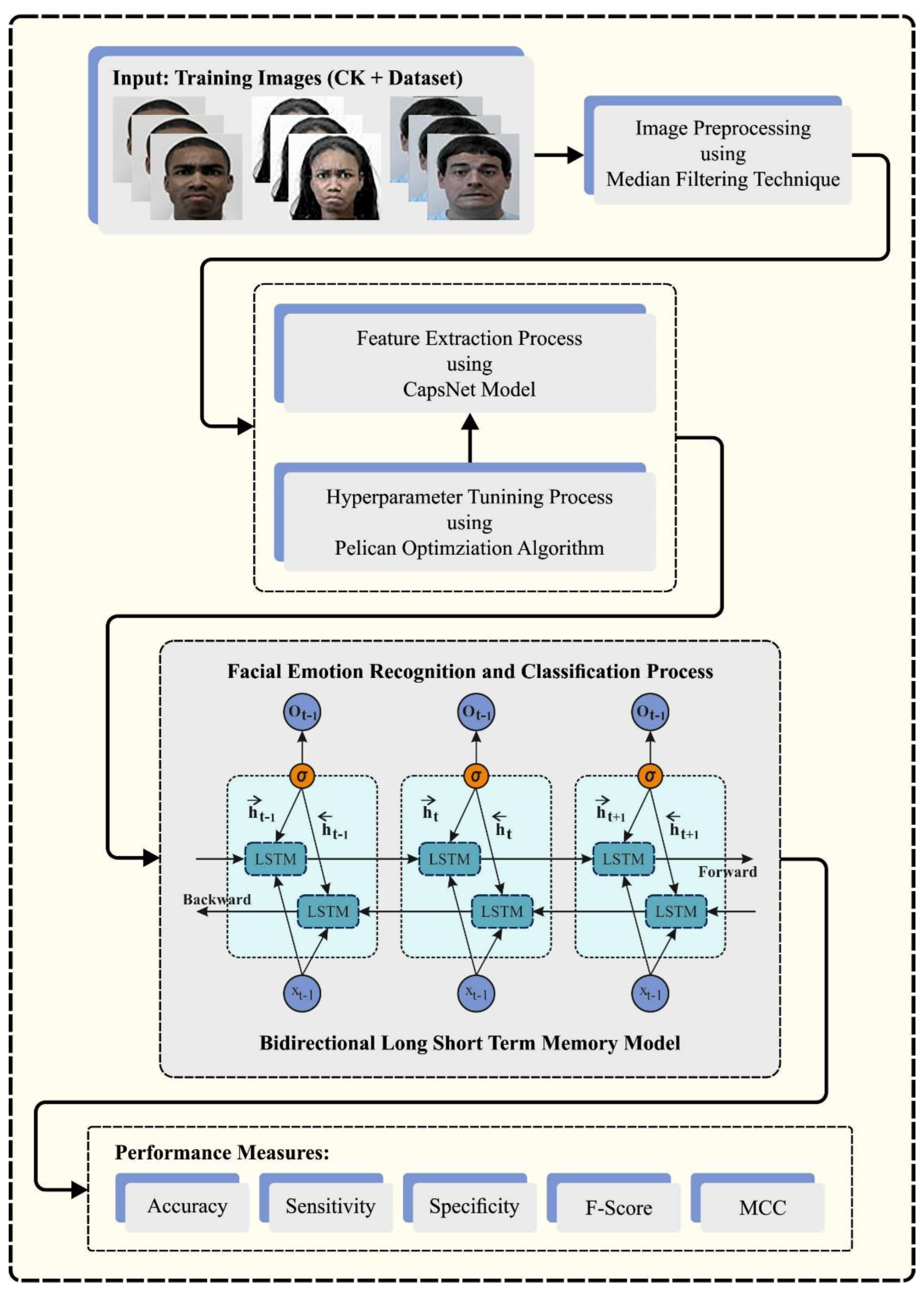
- An AFER-POADCNN technique comprising MF-based preprocessing, a CapsNet feature extractor, POA-based hyperparameter tuning, and BiLSTM classification has been developed for FER. To the best of our knowledge, the AFER-POADCNN technique has never existed in the literature;
- The CapsNet model has been employed for feature extraction, allowing for the capture of intricate and nuanced facial expressions;
- The POA is presented to tune the hyperparameters of the capsule network, enhancing the model’s adaptability and generalization to different emotions and diverse populations;
- The BiLSTM model applied for emotion classification ensures the robust detection and categorization of various facial emotions.
2. Literature Review
3. The Proposed Model
3.1. Image Preprocessing
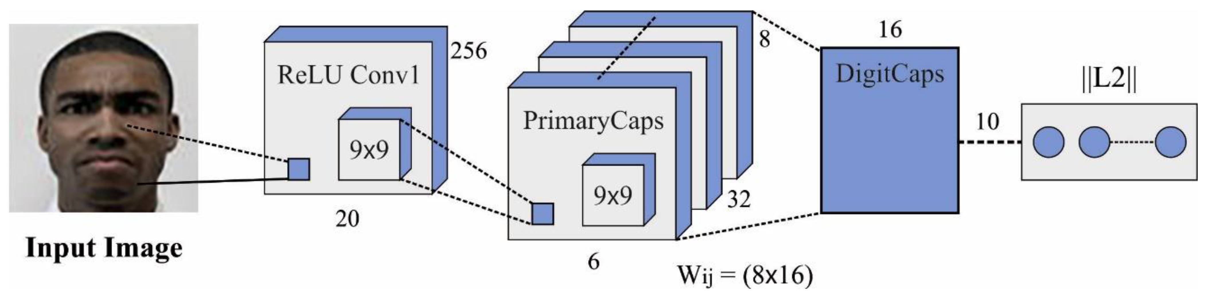
3.2. Feature Extraction
3.3. Hyperparameter Tuning
- 1.
- Exploration Stage (Moving direction of Bait)
- 2.
- Exploitation Stage (Winging on the Water Surface)
- 3.
- Repetition
3.4. Detection Using the BiLSTM Model
4. Results and Discussion
5. Conclusions
Author Contributions
Funding
Data Availability Statement
Conflicts of Interest
References
- Mukhiddinov, M.; Djuraev, O.; Akhmedov, F.; Mukhamadiyev, A.; Cho, J. Masked Face Emotion Recognition Based on Facial Landmarks and Deep Learning Approaches for Visually Impaired People. Sensors 2023, 23, 1080. [Google Scholar] [CrossRef]
- Gupta, S.; Kumar, P.; Tekchandani, R.K. Facial emotion recognition based real-time learner engagement detection system in online learning context using deep learning models. Multimed. Tools Appl. 2023, 82, 11365–11394. [Google Scholar] [CrossRef]
- Poulose, A.; Reddy, C.S.; Kim, J.H.; Han, D.S. Foreground Extraction Based Facial Emotion Recognition Using Deep Learning Xception Model. In 2021 Twelfth International Conference on Ubiquitous and Future Networks (ICUFN), Jeju Island, Republic of Korea, 17–20 August 2021; IEEE: New York, NY, USA, 2021; pp. 356–360. [Google Scholar]
- Gaddam, D.K.R.; Ansari, M.D.; Vuppala, S.; Gunjan, V.K.; Sati, M.M. Human facial emotion detection using deep learning. In Lecture Notes in Electrical Engineering, Proceedings of the ICDSMLA 2020: 2nd International Conference on Data Science, Machine Learning and Applications, Pune, India, 21–22 November 2020; Springer: Singapore, 2021; pp. 1417–1427. [Google Scholar]
- Hossain, S.; Umer, S.; Rout, R.K.; Tanveer, M. Fine-grained image analysis for facial expression recognition using deep convolutional neural networks with bilinear pooling. Appl. Soft Comput. 2023, 134, 109997. [Google Scholar] [CrossRef]
- Chaudhari, A.; Bhatt, C.; Krishna, A.; Travieso-González, C.M. Facial emotion recognition with inter-modality-attention-transformer-based self-supervised learning. Electronics 2023, 12, 288. [Google Scholar] [CrossRef]
- Sabour, S.; Frosst, N.; Hinton, G.E. Dynamic routing between capsules. In Advances in Neural Information Processing Systems 30, Proceedings of the Annual Conference on Neural Information Processing Systems, Long Beach, CA, USA, 4–9 December 2017; Neural Information Processing Systems Foundation, Inc. (NeurIPS): San Diego, CA, USA, 2017; pp. 3856–3866. [Google Scholar]
- Chen, H.; Wang, T.; Chen, T.; Deng, W. Hyperspectral image classification based on fusing S3-PCA, 2D-SSA and random patch network. Remote Sens. 2023, 15, 3402. [Google Scholar] [CrossRef]
- Duan, Z.; Song, P.; Yang, C.; Deng, L.; Jiang, Y.; Deng, F.; Jiang, X.; Chen, Y.; Yang, G.; Ma, Y.; et al. The impact of hyperglycaemic crisis episodes on long-term outcomes for inpatients presenting with acute organ injury: A prospective, multicentre follow-up study. Front. Endocrinol. 2022, 13, 1057089. [Google Scholar] [CrossRef]
- Bharti, S.K.; Varadhaganapathy, S.; Gupta, R.K.; Shukla, P.K.; Bouye, M.; Hingaa, S.K.; Mahmoud, A. Text-Based Emotion Recognition Using Deep Learning Approach. Comput. Intell. Neurosci. 2022, 2022, 2645381. [Google Scholar] [CrossRef]
- Lasri, I.; Riadsolh, A.; Elbelkacemi, M. Facial emotion recognition of deaf and hard-of-hearing students for engagement detection using deep learning. Educ. Inf. Technol. 2023, 28, 4069–4092. [Google Scholar] [CrossRef]
- Khattak, A.; Asghar, M.Z.; Ali, M.; Batool, U. An efficient deep learning technique for facial emotion recognition. Multimed. Tools Appl. 2022, 81, 1649–1683. [Google Scholar] [CrossRef]
- Durga, B.K.; Rajesh, V.; Jagannadham, S.; Kumar, P.S.; Rashed, A.N.Z.; Saikumar, K. Deep Learning-Based Micro Facial Expression Recognition Using an Adaptive Tiefes FCNN Model. Trait. Signal 2023, 40, 1035–1043. [Google Scholar] [CrossRef]
- Arora, T.K.; Chaubey, P.K.; Raman, M.S.; Kumar, B.; Nagesh, Y.; Anjani, P.K.; Ahmed, H.M.S.; Hashmi, A.; Balamuralitharan, S.; Debtera, B. Optimal facial feature-based emotional recognition using a deep learning algorithm. Comput. Intell. Neurosci. 2022, 2022, 8379202. [Google Scholar]
- Sarvakar, K.; Senkamalavalli, R.; Raghavendra, S.; Kumar, J.S.; Manjunath, R.; Jaiswal, S. Facial emotion recognition using convolutional neural networks. Mater. Today Proc. 2023, 80, 3560–3564. [Google Scholar] [CrossRef]
- Said, Y.; Barr, M. Human emotion recognition based on facial expressions via deep learning on high-resolution images. Multimed. Tools Appl. 2021, 80, 25241–25253. [Google Scholar] [CrossRef]
- Umer, S.; Rout, R.K.; Pero, C.; Nappi, M. Facial expression recognition with trade-offs between data augmentation and deep learning features. J. Ambient Intell. Humaniz. Comput. 2022, 13, 721–735. [Google Scholar] [CrossRef]
- Talaat, F.M. Real-time facial emotion recognition system among children with autism based on deep learning and IoT. Neural Comput. Appl. 2023, 35, 12717–12728. [Google Scholar] [CrossRef]
- Chowdary, M.K.; Nguyen, T.N.; Hemanth, D.J. Deep learning-based facial emotion recognition for human–computer interaction applications. Neural Comput. Appl. 2023, 35, 23311–23328. [Google Scholar] [CrossRef]
- Saeed, S.; Shah, A.A.; Ehsan, M.K.; Amirzada, M.R.; Mahmood, A.; Mezgebo, T. Automated facial expression recognition framework using deep learning. J. Healthc. Eng. 2022, 2022, 5707930. [Google Scholar] [CrossRef]
- Sikkandar, H.; Thiyagarajan, R. Deep learning-based facial expression recognition using improved Cat Swarm Optimization. J. Ambient Intell. Humaniz. Comput. 2021, 12, 3037–3053. [Google Scholar] [CrossRef]
- Helaly, R.; Messaoud, S.; Bouaafia, S.; Hajjaji, M.A.; Mtibaa, A. DTL-I-ResNet18: Facial emotion recognition based on deep transfer learning and improved ResNet18. Signal Image Video Process. 2023, 17, 2731–2744. [Google Scholar] [CrossRef]
- Thuseethan, S.; Rajasegarar, S.; Yearwood, J. Deep3DCANN: A Deep 3DCNN-ANN framework for spontaneous micro-expression recognition. Inf. Sci. 2023, 630, 341–355. [Google Scholar] [CrossRef]
- Kansizoglou, I.; Bampis, L.; Gasteratos, A. An active learning paradigm for online audio-visual emotion recognition. IEEE Trans. Affect. Comput. 2019, 13, 756–768. [Google Scholar] [CrossRef]
- Li, Y.; Gao, Y.; Chen, B.; Zhang, Z.; Lu, G.; Zhang, D. Self-supervised exclusive-inclusive interactive learning for multi-label facial expression recognition in the wild. IEEE Trans. Circuits Syst. Video Technol. 2021, 32, 3190–3202. [Google Scholar] [CrossRef]
- Kansizoglou, I.; Misirlis, E.; Tsintotas, K.; Gasteratos, A. Continuous emotion recognition for long-term behaviour modelling through recurrent neural networks. Technologies 2022, 10, 59. [Google Scholar] [CrossRef]
- Kumar, A.; Patel, V.K. Classification and identification of disease in potato leaf using hierarchical-based deep learning convolutional neural network. Multimed. Tools Appl. 2023, 82, 31101–31127. [Google Scholar] [CrossRef]
- Guo, X.; Ghadimi, N. Optimal Design of the Proton-Exchange Membrane Fuel Cell Connected to the Network Utilizing an Improved Version of the Metaheuristic Algorithm. Sustainability 2023, 15, 13877. [Google Scholar] [CrossRef]
- Nie, Q.; Wan, D.; Wang, R. CNN-BiLSTM water level prediction method with an attention mechanism. J. Phys. Conf. Ser. 2021, 2078, 012032. [Google Scholar] [CrossRef]
- Available online: http://www.jeffcohn.net/Resources/ (accessed on 14 July 2023).
- AlEisa, H.N.; Alrowais, F.; Negm, N.; Almalki, N.; Khalid, M.; Marzouk, R.; Alnfiai, M.M.; Mohammed, G.P.; Alneil, A.A. Henry Gas Solubility Optimization with Deep Learning Based Facial Emotion Recognition for Human-Computer Interface. IEEE Access 2023, 11, 62233–62241. [Google Scholar] [CrossRef]


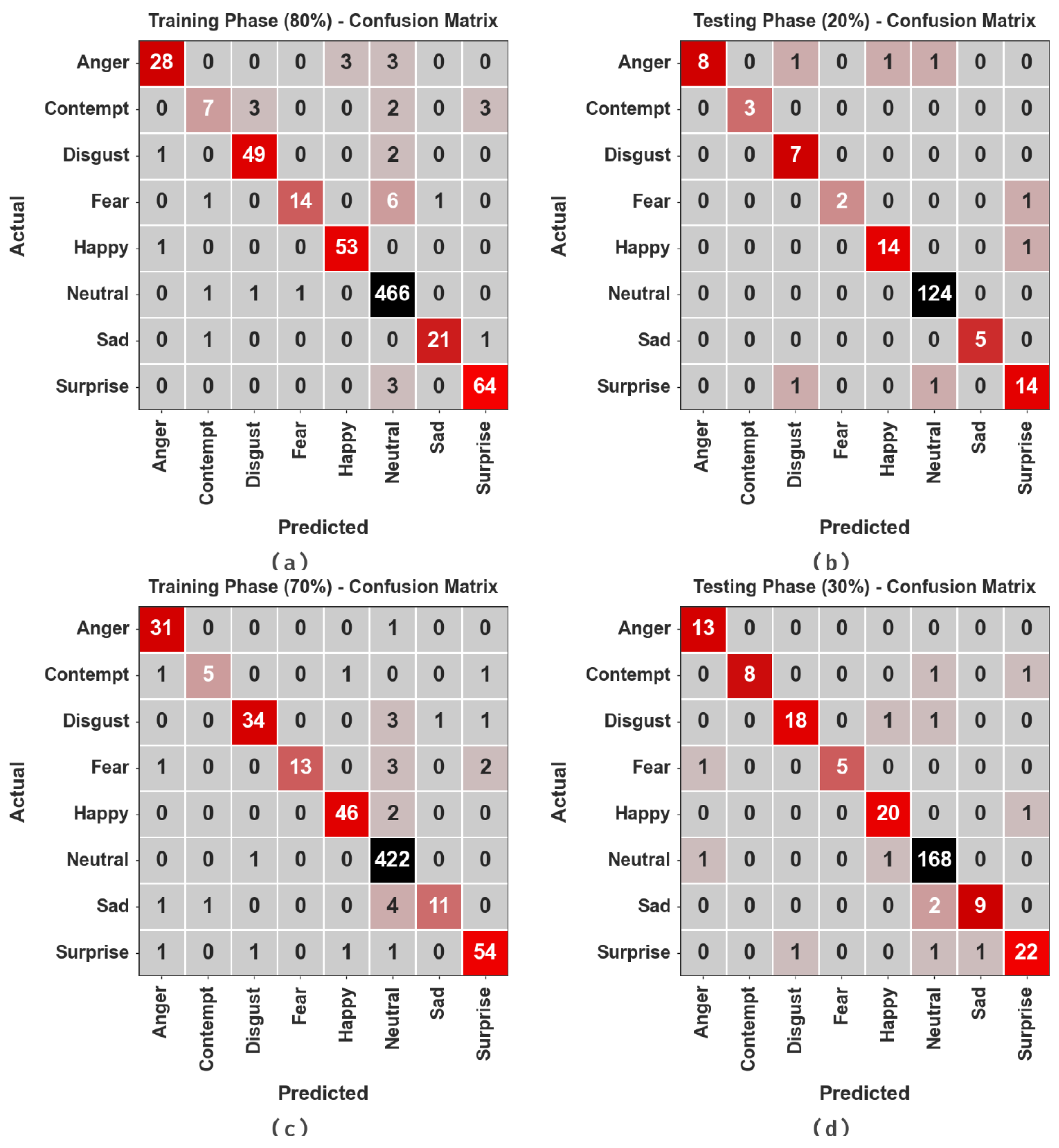
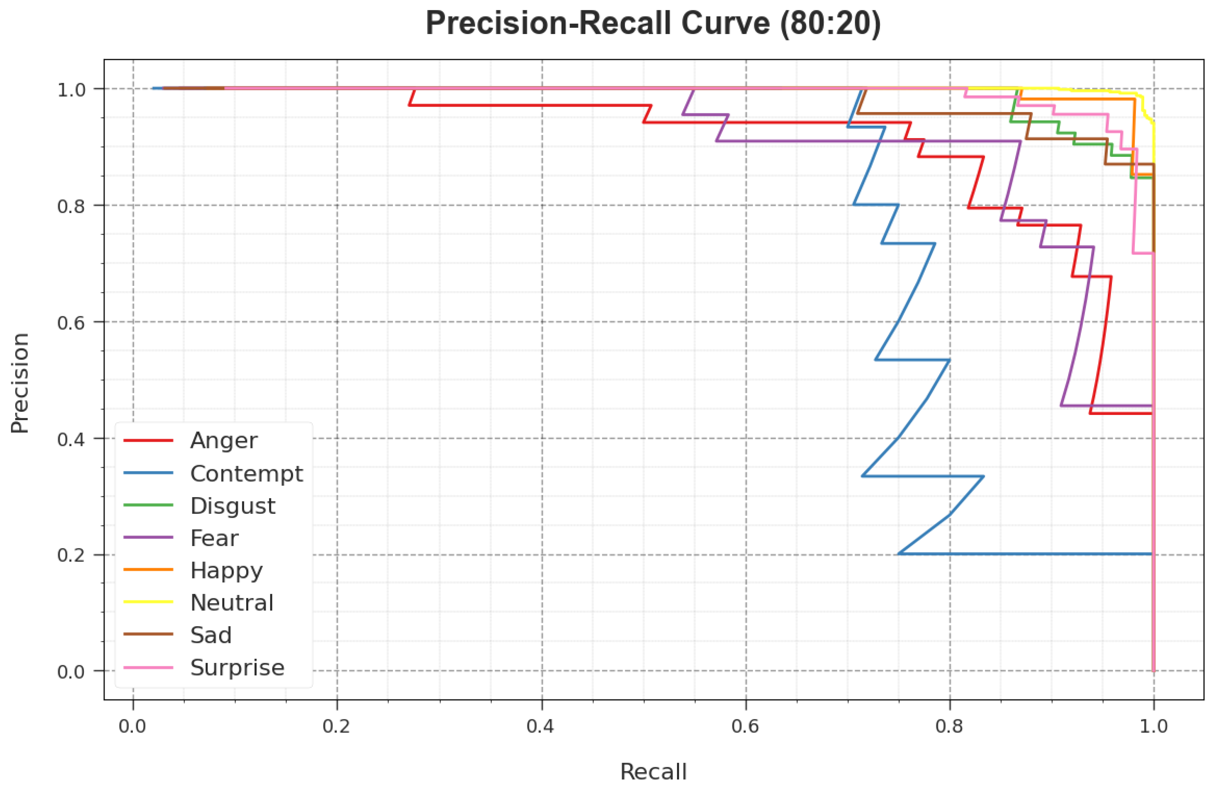
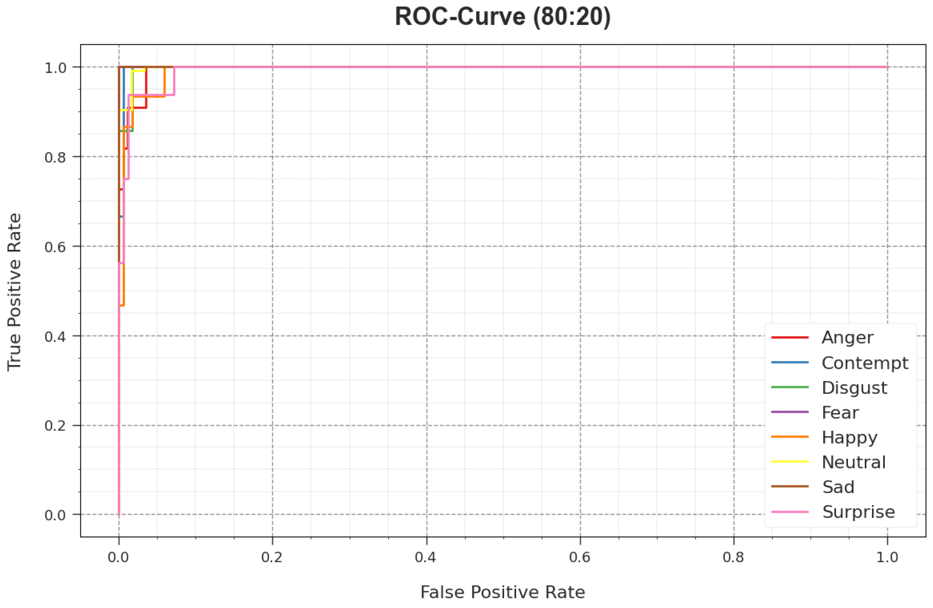
| Classes | No. of Samples |
|---|---|
| Anger | 45 |
| Contempt | 18 |
| Disgust | 59 |
| Fear | 25 |
| Happy | 69 |
| Neutral | 593 |
| Sad | 28 |
| Surprise | 83 |
| Total No. of Sample Images | 920 |
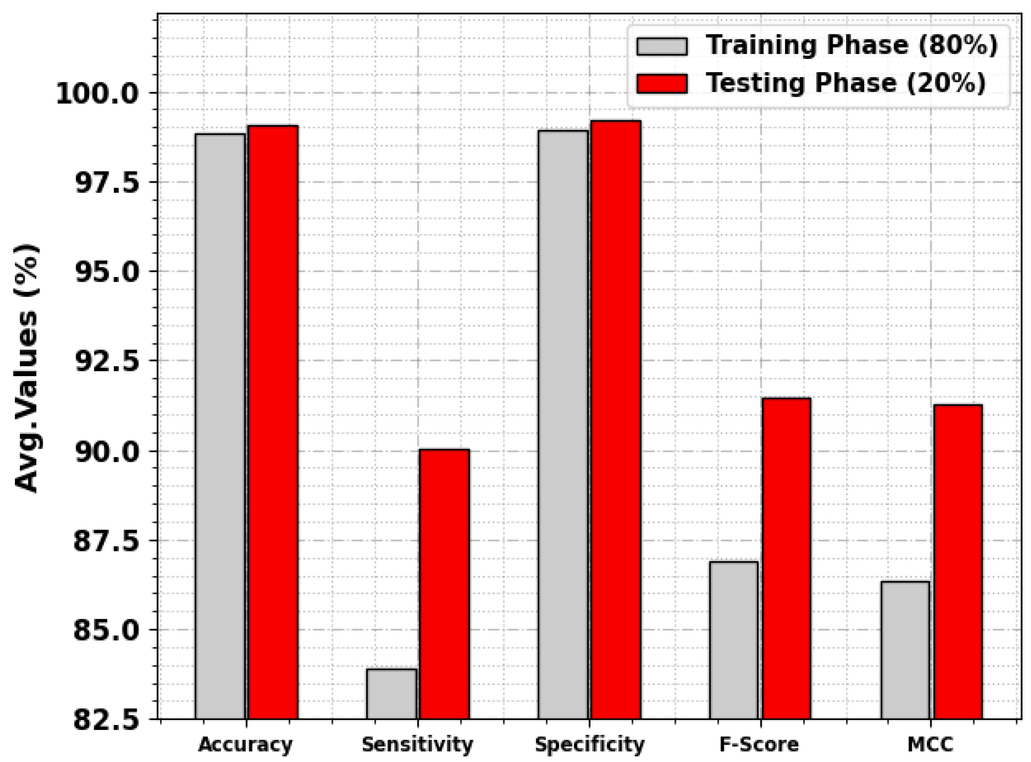
| Classes | MCC | ||||
|---|---|---|---|---|---|
| TR Phase (80%) | |||||
| Anger | 98.91 | 82.35 | 99.72 | 87.50 | 87.12 |
| Contempt | 98.51 | 46.67 | 99.58 | 56.00 | 56.45 |
| Disgust | 99.05 | 94.23 | 99.42 | 93.33 | 92.83 |
| Fear | 98.78 | 63.64 | 99.86 | 75.68 | 76.52 |
| Happy | 99.46 | 98.15 | 99.56 | 96.36 | 96.09 |
| Neutral | 97.42 | 99.36 | 94.01 | 98.00 | 94.43 |
| Sad | 99.59 | 91.30 | 99.86 | 93.33 | 93.15 |
| Surprise | 99.05 | 95.52 | 99.40 | 94.81 | 94.29 |
| Average | 98.85 | 83.90 | 98.93 | 86.88 | 86.36 |
| TS Phase (20%) | |||||
| Anger | 98.37 | 72.73 | 100.00 | 84.21 | 84.55 |
| Contempt | 100.00 | 100.00 | 100.00 | 100.00 | 100.00 |
| Disgust | 98.91 | 100.00 | 98.87 | 87.50 | 87.69 |
| Fear | 99.46 | 66.67 | 100.00 | 80.00 | 81.43 |
| Happy | 98.91 | 93.33 | 99.41 | 93.33 | 92.74 |
| Neutral | 98.91 | 100.00 | 96.67 | 99.20 | 97.54 |
| Sad | 100.00 | 100.00 | 100.00 | 100.00 | 100.00 |
| Surprise | 97.83 | 87.50 | 98.81 | 87.50 | 86.31 |
| Average | 99.05 | 90.03 | 99.22 | 91.47 | 91.28 |
| Classes | MCC | ||||
|---|---|---|---|---|---|
| TR Phase (70%) | |||||
| Anger | 99.22 | 96.88 | 99.35 | 92.54 | 92.23 |
| Contempt | 99.38 | 62.50 | 99.84 | 71.43 | 71.87 |
| Disgust | 98.91 | 87.18 | 99.67 | 90.67 | 90.17 |
| Fear | 99.07 | 68.42 | 100.00 | 81.25 | 82.32 |
| Happy | 99.38 | 95.83 | 99.66 | 95.83 | 95.50 |
| Neutral | 97.67 | 99.76 | 93.67 | 98.25 | 94.86 |
| Sad | 98.91 | 64.71 | 99.84 | 75.86 | 76.52 |
| Surprise | 98.76 | 93.10 | 99.32 | 93.10 | 92.42 |
| Average | 98.91 | 83.55 | 98.92 | 87.37 | 86.99 |
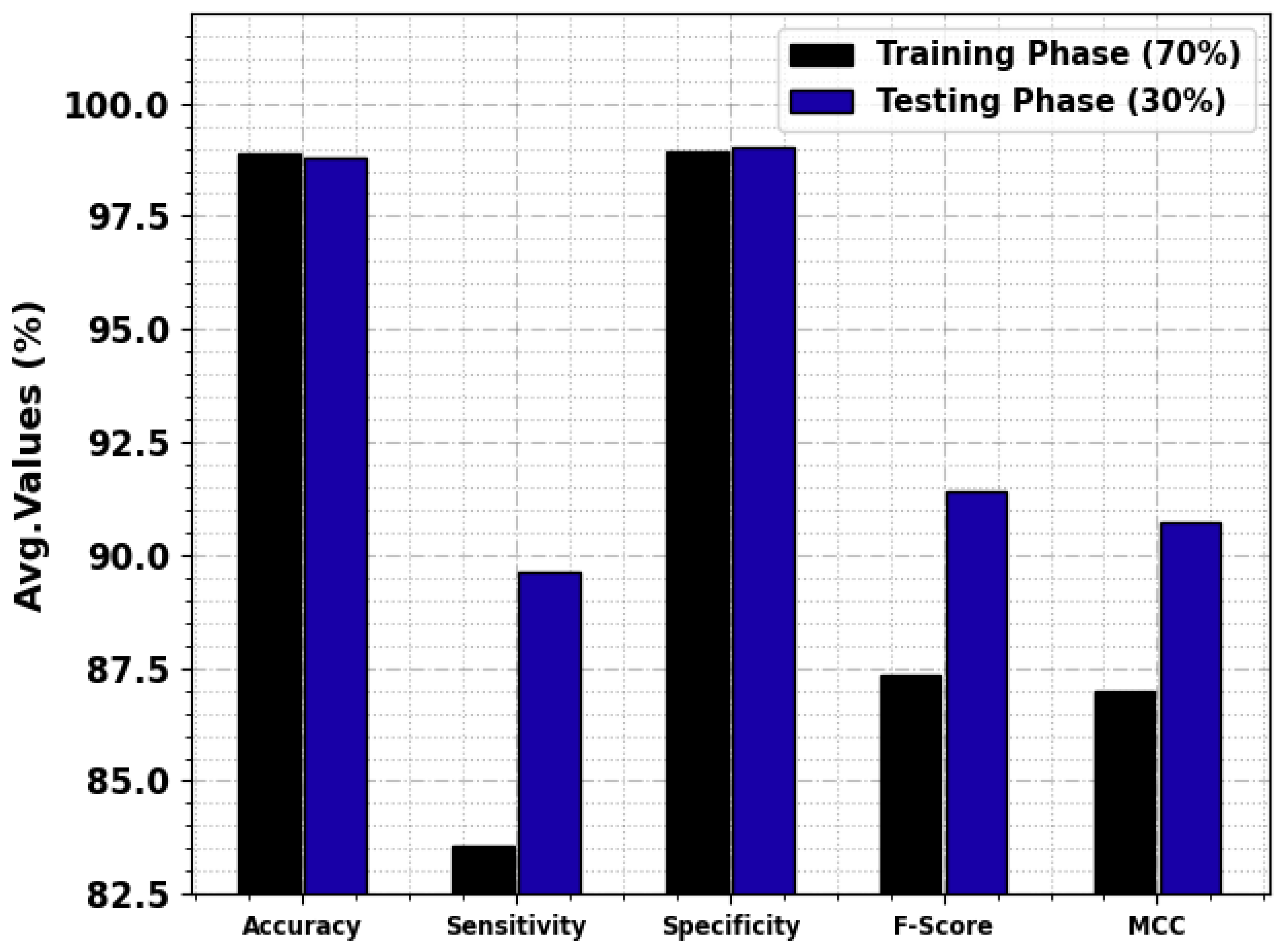
| TS Phase (30%) | |||||
| Anger | 99.28 | 100.00 | 99.24 | 92.86 | 92.74 |
| Contempt | 99.28 | 80.00 | 100.00 | 88.89 | 89.11 |
| Disgust | 98.91 | 90.00 | 99.61 | 92.31 | 91.76 |
| Fear | 99.64 | 83.33 | 100.00 | 90.91 | 91.12 |
| Happy | 98.91 | 95.24 | 99.22 | 93.02 | 92.46 |
| Neutral | 97.46 | 98.82 | 95.28 | 97.96 | 94.64 |
| Sad | 98.91 | 81.82 | 99.62 | 85.71 | 85.26 |
| Surprise | 98.19 | 88.00 | 99.20 | 89.80 | 88.82 |
| Average | 98.82 | 89.65 | 99.02 | 91.43 | 90.74 |
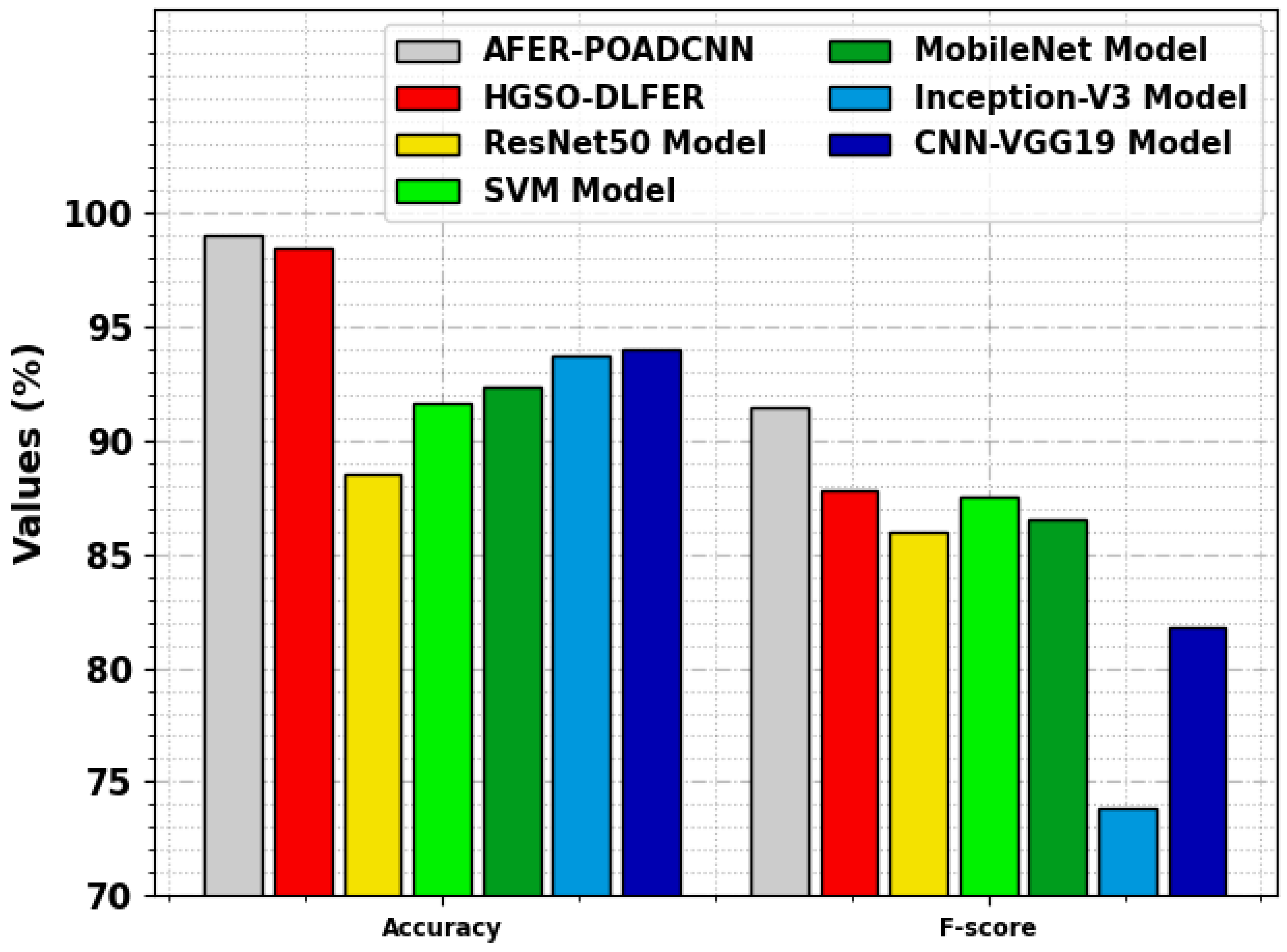
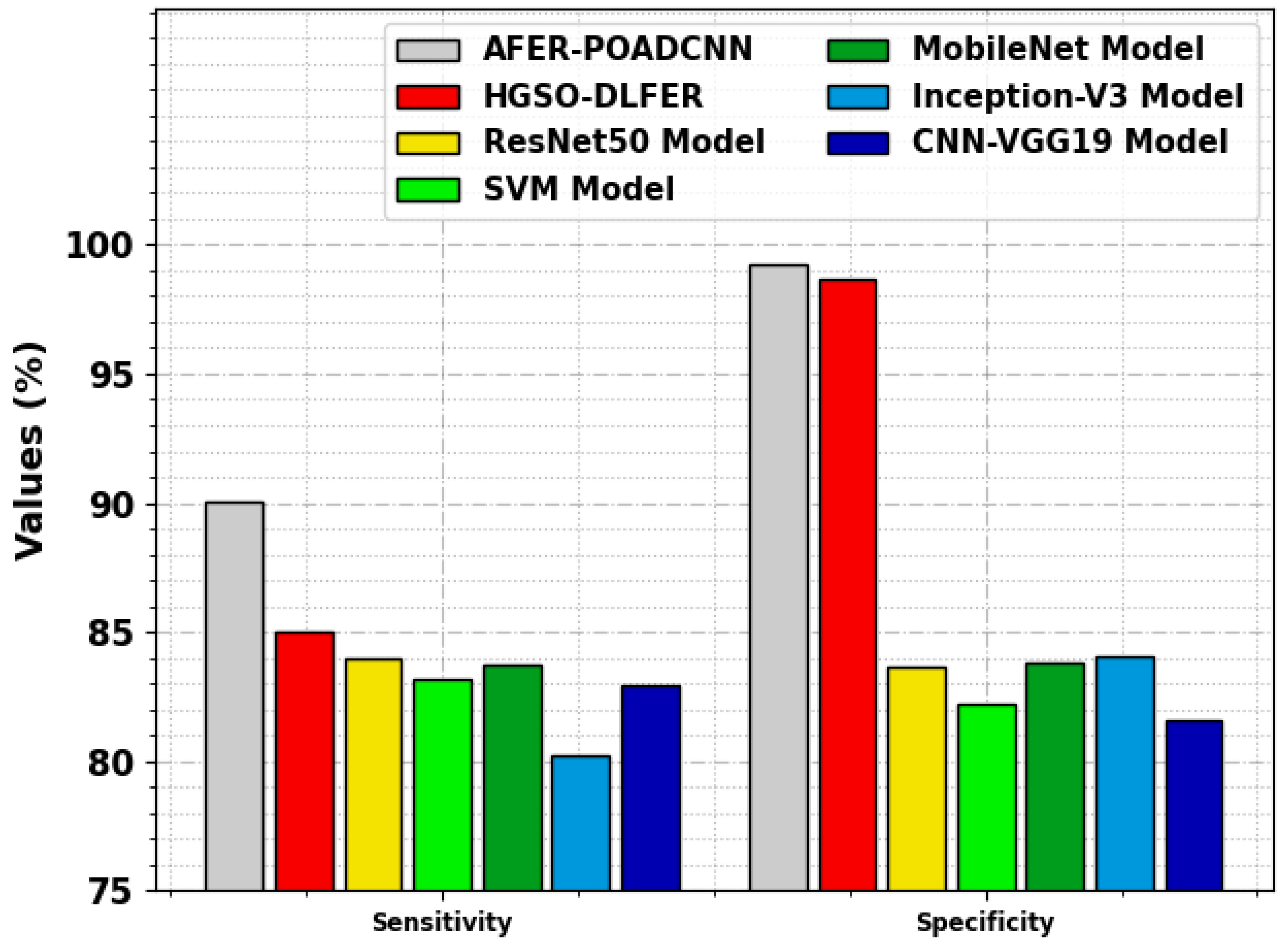
| Methods | ||||
|---|---|---|---|---|
| AFER-POADCNN | 90.03 | 99.22 | 99.05 | 91.47 |
| HGSO-DLFER | 84.99 | 98.65 | 98.45 | 87.78 |
| ResNet50 | 83.96 | 83.65 | 88.54 | 85.99 |
| SVM | 83.17 | 82.18 | 91.64 | 87.55 |
| MobileNet | 83.74 | 83.81 | 92.32 | 86.52 |
| Inception-V3 | 80.23 | 84.06 | 93.74 | 73.82 |
| CNN-VGG19 | 82.95 | 81.59 | 94.03 | 81.75 |
Disclaimer/Publisher’s Note: The statements, opinions and data contained in all publications are solely those of the individual author(s) and contributor(s) and not of MDPI and/or the editor(s). MDPI and/or the editor(s) disclaim responsibility for any injury to people or property resulting from any ideas, methods, instructions or products referred to in the content. |
© 2023 by the authors. Licensee MDPI, Basel, Switzerland. This article is an open access article distributed under the terms and conditions of the Creative Commons Attribution (CC BY) license (https://creativecommons.org/licenses/by/4.0/).
Share and Cite
Alonazi, M.; Alshahrani, H.J.; Alotaibi, F.A.; Maray, M.; Alghamdi, M.; Sayed, A. Automated Facial Emotion Recognition Using the Pelican Optimization Algorithm with a Deep Convolutional Neural Network. Electronics 2023, 12, 4608. https://doi.org/10.3390/electronics12224608
Alonazi M, Alshahrani HJ, Alotaibi FA, Maray M, Alghamdi M, Sayed A. Automated Facial Emotion Recognition Using the Pelican Optimization Algorithm with a Deep Convolutional Neural Network. Electronics. 2023; 12(22):4608. https://doi.org/10.3390/electronics12224608
Chicago/Turabian StyleAlonazi, Mohammed, Hala J. Alshahrani, Faiz Abdullah Alotaibi, Mohammed Maray, Mohammed Alghamdi, and Ahmed Sayed. 2023. "Automated Facial Emotion Recognition Using the Pelican Optimization Algorithm with a Deep Convolutional Neural Network" Electronics 12, no. 22: 4608. https://doi.org/10.3390/electronics12224608
APA StyleAlonazi, M., Alshahrani, H. J., Alotaibi, F. A., Maray, M., Alghamdi, M., & Sayed, A. (2023). Automated Facial Emotion Recognition Using the Pelican Optimization Algorithm with a Deep Convolutional Neural Network. Electronics, 12(22), 4608. https://doi.org/10.3390/electronics12224608