Article

Enhancing Multi-Objective Optimization with Automatic Construction of Parallel Algorithm Portfolios

1
School of Mechanical Engineering, University of Science and Technology Beijing, Beijing 100083, China
2
Beijing Key Laboratory of Research and Application for Robotic Intelligence of Hand-Eye-Brain Interaction, Beijing 100190, China
3
Centre for Frontier AI Research, Agency for Science, Technology and Research, Singapore 138632, Singapore
4
Department of Computer Science and Engineering, Southern University of Science and Technology, Shenzhen 518055, China
*
Author to whom correspondence should be addressed.
Electronics 2023, 12(22), 4639; https://doi.org/10.3390/electronics12224639
Submission received: 9 October 2023 / Revised: 8 November 2023 / Accepted: 9 November 2023 / Published: 13 November 2023
(This article belongs to the Section Artificial Intelligence)

Abstract

:
It has been widely observed that there exists no universal best Multi-Objective Evolutionary Algorithm (MOEA) dominating all other MOEAs on all possible Multi-Objective Optimization Problems (MOPs). In this work, we advocate using the Parallel Algorithm Portfolio (PAP), which runs multiple MOEAs independently in parallel and gets the best out of them, to combine the advantages of different MOEAs. Since the manual construction of PAPs is non-trivial and tedious, we propose to automatically construct high-performance PAPs for solving MOPs. Specifically, we first propose a variant of PAPs, namely MOEAs/PAP, which can better determine the output solution set for MOPs than conventional PAPs. Then, we present an automatic construction approach for MOEAs/PAP with a novel performance metric for evaluating the performance of MOEAs across multiple MOPs. Finally, we use the proposed approach to construct an MOEAs/PAP based on a training set of MOPs and an algorithm configuration space defined by several variants of NSGA-II. Experimental results show that the automatically constructed MOEAs/PAP can even rival the state-of-the-art multi-operator-based MOEAs designed by human experts, demonstrating the huge potential of the automatic construction of PAPs in multi-objective optimization.

1. Introduction

Multi-Objective Optimization Problems (MOPs) are a class of classical optimization problems, which widely exist in many real-world applications such as finance [1], vehicle routing [2], and adversarial attack [3]. Multi-Objective Evolutionary Algorithms (MOEAs), as a kind of algorithm for solving MOPs, have attracted great attention over the past few decades and have shown a good performance [4,5,6,7,8,9,10]. Generally, MOEAs follow the generational framework where a population of solutions evolve from one generation to the next. In the evolution process, evolutionary operators (e.g., mutation and crossover) are used to generate offspring through the parents, while environmental selection operators are used to select elite individuals for the next-generation evolution.
Despite the tremendous success achieved by MOEAs, it has been widely observed [11,12,13,14] that there exists no universal best MOEA that dominates over all other MOEAs on all possible MOPs. Instead, different MOEAs are good at solving different MOPs due to their abilities on exploitation and exploration [15]. For example, MOEAs equipped with polynomial-based mutation (PM) [16] are good at searching in a local area, while those using simulated binary crossover (SBX) [17] and differential evolution (DE) [18,19] are capable of exploring the search space globally. Hence, in order to achieve a better overall performance for a diverse range of MOPs, it is natural and intuitive to combine the advantages of different MOEAs. One notable series of research efforts following this idea are multi-operator-based MOEAs [11,12,13,14], which adaptively allocate computational resources to MOEAs equipped with different operators when solving a MOP.
Apart from multi-operator-based MOEAs, and from a more general perspective of problem solving, there is an effective technique that exploits the complementarity between different algorithms by including them into a so-called algorithm portfolio (AP). To utilize an AP to solve a problem, Tang et al. [20,21] proposed a simple but effective strategy, called a parallel algorithm portfolio (PAP), that runs all member algorithms in the portfolio independently in parallel to obtain multiple solutions. Then, the best solution will be taken as the final output of the PAP. Although a PAP would consume more computational resources than a single algorithm, it has three important advantages. First, PAPs are easy-to-implement because they do not necessarily require any resource allocation since each member algorithm is simply assigned with the same amount of resource. Second, the performance of a PAP on any problem is the best performance achieved among its member algorithms on the problem. In other words, a PAP could achieve a much better overall performance than any of its member algorithms. Third, considering the tremendous growth of parallel computing architectures [22] (e.g., multi-core CPUs) over the last few decades, leveraging parallelism has become very important in designing effective solvers for hard optimization problems [23,24,25,26,27]. PAPs employ parallel solution strategies and thus allow for the use of modern computing facilities in an extremely simple way.
It is conceivable that any PAP’s effectiveness relies heavily on the diversity and complementarity among its member algorithms. In other words, the manual construction of high-quality PAPs is generally a challenging task, requiring domain experts (with a deep understanding of both algorithms and problems) to explore the vast design space of PAPs, which cannot be carried out manually with ease [28,29,30]. As an alternative, Tang and Liu [25,26] proposed a general framework, called automatic construction of PAPs, that seeks to automatically build PAPs by selecting the member algorithms from an algorithm configuration space, with the goal of optimizing the performance of the resulting PAP on a given problem set (called training set). Such a framework has been shown to be effective in building high-performance PAPs for combinatorial problems such as the Boolean Satisfiability Problem (SAT) [25], the Traveling Salesman Problem (TSP) [27,31], and the Vehicle Routing Problem (VRP) [26].
However, to the best of our knowledge, the potential of the automatic construction of PAPs has not been investigated in the area of multi-objective optimization. Considering its excellent performance on the above-mentioned problems and the practical significance of MOPs, studying how to utilize it to solve MOPs is thus valuable. In this work, we focus on automatically building PAPs for continuous MOPs. On the other hand, as a general framework, appropriately instantiating automatic PAP construction for a specific problem domain is non-trivial. Specifically, it requires careful designs of the algorithm configuration space and the performance metrics used in the construction process [26].
The main contributions of this work can be summarized as follows.
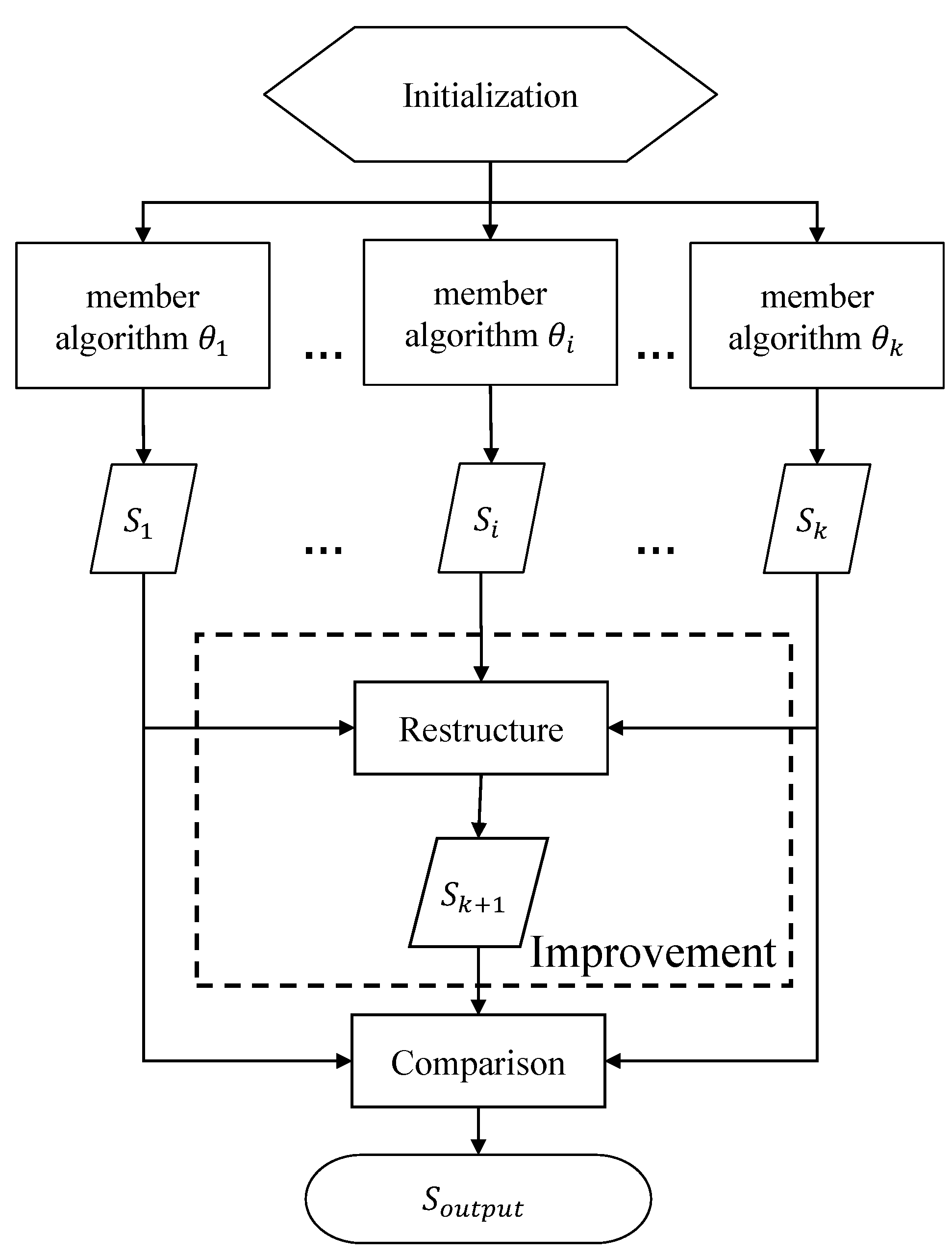
  • Taking the characteristics of MOPs into account, we propose a novel variant form of PAP for MOPs, dubbed MOEAs/PAP. Its main difference from conventional PAPs lies in the method for determining the final output. MOEAs/PAP would compare the solution sets found by member algorithms and the solution set generated based on all the solutions found by member algorithms, and finally output the best solution set.
  • We present an automatic construction approach for MOEAs/PAP with a novel metric that evaluates the performance of MOEAs/PAPs across multiple MOPs.
  • Based on a training set of MOPs and an algorithm configuration space defined by several variants of NSGA-II, we use the proposed approach to construct an MOEAs/PAP, namely NSGA-II/PAP. Experimental results show that NSGA-II/PAP significantly outperforms existing single-operator-based MOEAs and the state-of-the-art multi-operator-based MOEAs designed by human experts. Such promising results indicate the huge potential of automatic construction of PAPs in multi-objective optimization.
The remainder of this paper is organized as follows. Section 2 presents the preliminaries and briefly reviews the related works. Section 3 gives the variant form of PAP for MOPs. The automatic construction approach, as well as the algorithm configuration space, the training set, and the performance metric used in construction, are presented in Section 4. Section 5 presents the experimental study. Finally, Section 6 concludes the paper.

2. Preliminaries and Related Work

2.1. Multi-Objective Optimization Problems

Without loss of generality, in this work we assume optimization problems take the minimization form. MOPs are optimization problems with multiple objectives, defined as follows:
min F ( x ) = [ f 1 ( x ) , f 2 ( x ) , , f m ( x ) ] Π x = [ x 1 , x 2 , , x n ] D ,
where x is the decision vector, which consists of n decision variables. The objective vector F : D Π consists of m objectives; D R n and Π R m denote the decision space and the objective space, respectively. The objectives in Equation (1) are often in conflict with each other. That is, the improvement of one objective may lead to the deterioration of another. This gives rise to a set of optimal solutions (largely known as Pareto-optimal solutions), instead of a single optimal solution. The concept of Pareto-optimal is defined as follows.
Definition 1. 
Given two decision vectors u , v and their corresponding objective vectors F ( u ) , F ( v ) . u dominates v (denoted as u v ), if and only if i { 1 , , m } , f i ( u ) f i ( v ) and i { 1 , , m } , f i ( u ) < f i ( v ) .
Definition 2. 
A solution x * is Pareto-optimal if and only if there exists no u Ω such that u x * . The set of all Pareto-optimal solutions is called the Pareto set. The corresponding objective vector set of the Pareto set is called the Pareto front.
There exists a large body of benchmark sets for MOPs. Among them, Zizler–Deb–Thiele (ZDT) [32], Deb–Thiele–Laumanns–Zizler (DTLZ) [33], walking-fish-group (WFG) [34], and CEC 2009 competitions (UF) [35] are commonly used in the literature. These problems are characterized by multimodality, co-replicated Pareto sets and Pareto fronts, separability between decision variables, and correlation between decision variables and objectives, deception, and epistasis [34]. These are of varying difficulty and complexity and cover a variety of real-world problems. Moreover, the commonly used metrics for evaluating the solutions on MOPs include Inverted Generational Distance (IGD) [36] and Hypervolume (HV) [37,38].

2.2. Multi-Objective Evolutionary Algorithms

There is a large body of MOEAs, such as NSGA-II [4], MOEA/D [5], SPEA2 [8], PAES [10], and EMOCA [39]. This article will mainly introduce Genetic Algorithms (GAs) [4,5] and Differential Evolution (DE) Algorithms [40], and propose our algorithm based on these. GA is based on biological inspiration and generates new offspring by imitating the crossover and mutation process in biological genetic evolution. One of the most classic and widely used variation strategies is composed of a simulated binary crossover (SBX) operator and a polynomial mutation (PM) operator [41]. Specifically, supposing the two parent individuals are x 1 = ( x 1 1 , x 2 1 , , x n 1 ) and x 2 = ( x 1 2 , x 2 2 , , x n 2 ) , and the generated offspring are c 1 = ( c 1 1 , c 2 1 , , c n 1 ) and c 2 = ( c 1 2 , c 2 2 , , c n 2 ) . SBX and PM operate as follows.
SBX:
c i 1 = 0.5 × [ ( 1 + β ) · x i 1 + ( 1 β ) · x i 2 ] c i 2 = 0.5 × [ ( 1 β ) · x i 1 + ( 1 + β ) · x i 2 ] ,
where β is a parameter, defined as follows:
β = ( r × 2 ) 1 / ( 1 + η ) if r 0.5 ( 1 / ( 2 r × 2 ) ) 1 / ( 1 + η ) otherwise ,
where r is a random value within [ 0 , 1 ] and η is a parameter representing the similarity between the offspring individual and the parent individual. The larger the value, the higher the similarity.
PM:
c i 1 = x i 1 + Δ · ( u i l i ) ,
Δ is defined as follows:
Δ = ( 2 r + ( 1 2 r ) δ 1 η + 1 ) 1 / ( η + 1 ) 1 1 if r 0.5 ( ( 4 r 1 ) + ( 2 r 1 ) δ 2 η + 1 ) 1 / ( η + 1 ) otherwise ,
where δ 1 = ( u i x i 1 ) / ( u i l i ) and δ 2 = ( x i 1 l i ) / ( u i l i ) , r is a random parameter within [0, 1], u i and l i are the upper and lower bounds of the i-th dimension variable, respectively. η is a parameter that representing the similarity between the offspring individual and the parent individual. The larger the value, the higher the similarity.
rand/p:
c j i = x j r 3 + F · l = 1 p ( x j r 1 , l x j r 2 , l ) if r C R or j = j r x j i , otherwise ,
best/p:
c j i = x j b e s t + F · l = 1 p ( x j r 1 , l x j r 2 , l ) , if r C R or j = j r x j i , otherwise ,
current-to-rand/p:
c j i = x j i + K · ( x j r 3 x j i ) + F · l = 1 p ( x j r 1 , l x j r 2 , l ) if r C R or j = j r x j i otherwise ,
current-to-best/p:
c j i = x j i + K · ( x j b e s t x j i ) + F · l = 1 p ( x j r 1 , l x j r 2 , l ) , if r C R o r j = j r x j i , otherwise .
Different from GAs, DEs mainly perform gradient estimation through differential mutation operators to generate offspring. Over the past few decades, various types of differential mutation operators have been proposed. Mezura-Montes et al. [40] summarized them in Equations (6)–(9):
In Equations (6)–(9), p is the number of pairs of solutions used to compute the differences in the mutation operator, c j i is the j-th dimension variable of the i-th offspring, x j r 3 is the j-th dimension variable of the donor solution chosen at random, x j b e s t is the j-th dimension variable of the best solution in the population as the donor solution, x j i is the j-th dimension variable of the current parent, x j r 1 , l and x j r 2 , l are the j-th dimension variables of the p-th pair to compute the mutation differential, and F, K, and  C R are parameters in the DE algorithm.

2.3. Multi-Operator-Based MOEAs

Multi-Operator MOEAs mainly adaptively allocate the computation resources (population sizes) among different operators. The allocation strategy could be designed by human experts [11,12] or learned automatically [13,14]. Specifically, motivated by the well-known ensemble learning approach AdaBoost [42], Wang et al. [11] proposed to use the accumulated data of previous generations to adjust the population size of each operator in the next generation, such that the operators that produce better solutions in the previous generation will occupy more computational resources. Gao et al. [12] took the solutions generated by multiple operators as a whole and determined the local search strategy, global search direction, and final convergence direction by analyzing the features in the entire target space. Elsayed et al. [13] constructed a solver that includes two complementary algorithms. The inferior algorithm optimizes itself by learning the strategy of the superior algorithm and gives feedback to finetune the superior algorithm. Finally, the desired result is output from the high-quality algorithm. Sun et al. [14] regarded the parameter adaptation process as a Markov Decision Process (MDP). Through reinforcement learning, different parameter controllers are learned for different problems, such that they have different adaptive parameter selection methods for these problems. All of the above methods need a well-designed adaptive method to allocate computational resources to the member algorithms.

2.4. PAPs and Automatic Construction of PAPs

Essentially, a PAP [27,31,43] is a set of member algorithms that run in parallel:
P = θ 1 , θ 2 , , θ k ,
where P is the PAP solver, θ i is the i-th member algorithm of P, and k is the number of member algorithms.
Let M e t r i c ( θ , z ) denote the performance of an algorithm θ on a problem z (e.g., an MOP) in terms of the performance metric M e t r i c (e.g., HV for MOPs). Then, the performance of P on a problem z, denoted as Ω ( P , z ) , is the best performance achieved among the member algorithms of P on z:
Ω ( P , z ) = max θ P M e t r i c ( θ , z ) .
Without loss of generality, we assume for M, the larger the better. Let Z denote a set of problems. The performance of P on Z, denoted as Ω ( P , Z ) , is an aggregated value of the performance of P on all the problems in Z:
Ω ( P , Z ) = 1 | Z | · z Z Ω ( P , z ) .
The conventional way to construct P is to manually choose member algorithms for it, as shown in [20,21], which is, however, non-trivial and tedious. To address this issue, Tang and Liu [25,26] proposed the framework of the automatic construction of PAPs. Specifically, given a performance metric M e t r i c , a training set Z, and an algorithm configuration space Θ , the goal is to find at most k algorithms from Θ to form a PAP P * , which has the best performance on Z in terms of M:
P * = arg max P Θ & | P | k Ω ( P , Z ) ,
where Ω ( P , Z ) is defined in Equation (12). The results in [25,26,27,31] have shown that the PAPs automatically built by solving the problem in Equation (13) could achieve excellent performance on problems including SAT, TSPs, and VRPs, which are even better than the algorithms designed by human experts.

3. MOEAs/PAP for MOPs

As stated in Equation (11), a PAP would return the best solution among the ones found by its member algorithms. However, this could be problematic in multi-objective optimization since an MOEA outputs a set of Pareto-optimal solutions, instead of a single one, for a given MOP. One way to mitigate this issue is to compare the solution sets found by the member algorithms in terms of the performance metric (e.g., HV), and finally returns the best solution set.
On the other hand, it is likely that the solution sets found by member algorithms contain solutions that do not dominate each other. Thus, we propose a novel procedure called Restructure to obtain the final solution set. Specifically, when all member algorithms have completed their execution, the Pareto-optimal solution sets obtained by them are first combined. Assuming each member algorithm has a population size of P, the size of this set is N · P (N is the number of member algorithms). Then, Restructure employs the non-dominated sorting mechanism of NSGA-II [4] on these solutions and finally selects the top-P solutions to form the output solution set. Finally, all the solution sets found by member algorithms, as well as the one generated by Restructure, are compared, and the best set is returned as the output of MOEAs/PAP, as illustrated in Figure 1.
Formally, for an MOEAs/PAP, denoted as P, its performance on an MOP z can be described as follows:
Ω ( P , z ) = max { max θ P M e t r i c ( θ , z ) , M e t r i c ( θ ¯ , z ) } ,
where θ ¯ represents the Restructure procedure. Note Equation (14) is slightly different from Equation (11) (i.e., the performance of conventional PAPs) due to the Restructure procedure.

4. Automatic Construction of MOEAs/PAP

As aforementioned, the member algorithms of a PAP could be automatically determined by solving the problem defined in Equation (13). Below, we first introduce the algorithm configuration space Θ , the training set Z, and the performance metric M e t r i c ; then we present the automatic construction approach for MOEAs/PAP.

4.1. Algorithm Configuration Space Θ and Training Set Z

The algorithm configuration space Θ is defined by a number of parameterized algorithms B 1 , B 2 , , B c (called foundation algorithms). Each foundation algorithm B i has a number of parameters, whose values control the behavior of B i and thus can largely affect its performance. Therefore, B i taking different parameter values can actually be considered as different algorithms. Let Θ i denote the set of all unique algorithms obtained by taking all possible values of the parameters of B i . Then, the algorithm configuration space Θ is the union of Θ 1 , Θ 2 , , Θ c , i.e.,  Θ = Θ 1 Θ 2 Θ c . In this work, the foundation algorithms are parameterized MOEAs, i.e., NSGA-II with different evolutionary operators. The training set Z is a set of problems (MOPs), and should be representative of the target problems to which the constructed MOEAs/PAP is expected to be applied. The details of the algorithm configuration space Θ and the training set Z are given in the experiments (see Section 5.1 and Section 5.2).

4.2. Performance Metric

As stated in Equation (12), during the construction process, the performance of the PAP on the training set Z is an aggregated value of its performance on all the problems in Z. However, for MOPs, the commonly used IGD and HV cannot be directly used as the performance metric M e t r i c here. The main reason is that, for these two metrics, the performance of an MOEA on different MOPs cannot be directly aggregated (or compared) due to the different scales.
Hence, we propose to re-scale HV values within [ 0 , 1 ] , by using the following HV Ratio (HVR):
h v r = h v h v * ,
where h v is the HV value of the solution set found by an MOEA on an MOP, and  h v * is the HV value of the optimal solution set of the problem. Both h v and h v * are calculated based on the same reference point in the objective space, which is obtained by taking the maximum on each objective achieved among the solution set found by the MOEA. However, there is still an issue in the actual use of HVR. During the construction process of MOEAs/PAP, there is a large body of MOEAs, which would be evaluated. Since the reference point is up to the solution set found by the evaluated MOEA, given an MOP, h v * needs to be recalculated for every evaluated MOEA. Considering the size of the optimal solution set is usually very large (typically larger than 1000), thus in the construction process it requires a large amount of calculations for h v * .
To address the above issue, we propose to use a fixed reference point for a given MOP, such that h v * needs to be calculated for the problem for only once. One way is to use the the reference point taking the upper bounds (note that we assume MOPs take the minimization form) of the objective values. However, this will cause the gap between h v and h v * to be very small, in which case h v r tends to be 1 and loses its evaluation ability. Therefore, we calculate the HVs of the undominated space for the found solution set and the optimal solution set, and finally use the ratio of them to assess the performance of an MOEA on a MOP.
The new performance metric is named Inverted Hypervolume Ratio (IHVR):
i h v r = h v a l l h v * h v a l l h v ,
where h v and h v * are calculated based on the reference point taking the upper bounds of the objective values, and  h v a l l is the HV of the cube formed by the ranges of objective values of the MOP. Thus, h v a l l h v and h v a l l h v * are the HVs of the undominated space for the solution set found by the evaluated MOEA and the optimal solution set, respectively. Note that i h v r ( 0 , 1 ] , and a larger value of i h v r is better. IHVR can distinguish well between MOEAs with a different performance, and can also save a lot of calculations. In this work, IHVR is used as the performance metric M e t r i c .

4.3. Automatic Construction Approach

Algorithm 1 presents the automatic construction approach for MOEAs/PAP. Starting from an empty set (line 2), the approach constructs the PAP (denoted as P) iteratively. Specifically, each iteration of the approach (lines 3–15) consists of two subsequent phases. In the first phase, an existing automatic algorithm configuration tool, namely SMAC 3 [44], is used to search in Θ to find the algorithm that can improve the performance of the current PAP to the largest extent (line 5), and then this algorithm is inserted into P (line 6). This phase is similar to the commonly-used greedy approach in the automatic construction of PAPs [27,31]. Additionally, we introduce a new phase, namely simplification, as the second phase in Algorithm 1. In this phase (lines 7–14), P would be simplified by removing the member algorithms that do not contribute at all to its performance (meaning removing these algorithms has no effect on the performance of P on the training set). Considering the size of P is bounded (line 3), removing the redundant algorithms from P is meaningful because this will leave space for new member algorithms that can improve the performance of P. Finally, the approach would be terminated if the maximum number of member algorithms is reached (line 3), or the performance of P does not improve with the inclusion of the found algorithm (line 6).
Algorithm 1: Automatic construction of MOEAs/PAP.
  input
Algorithm configuration space Θ , training set Z, maximum number of member algorithms k
  output
the final PAP P
Electronics 12 04639 i001
(

5. Experiments

In the experiments, we first used the proposed automatic construction approach to build a MOEAs/PAP with a training set, and then compared it with other MOEAs on the testing set to verify its performance. Finally, we analyzed the performance of each member algorithm of the MOEAs/PAP, as well as the impact of the Restructure procedure.

5.1. Benchmark Sets

We collected the commonly-used MOP benchmarks in the literature, including ZDT [32], DTLZ [33], WFG [34], and UF [35]. These benchmark sets contain 32 MOPs in total, as summarized in Table 1. From each of these benchmark sets, several problems were chosen as the training problems, and the remaining problems were used for testing. Specifically, the training set includes 17 MOPs in total, i.e., ZDT3-6, DTLZ2-5, WFG1, WFG5-6, WFG9, UF3-4, UF6-7, and UF10; the testing set contains 15 MOPs in total, i.e., ZDT1-2, DTLZ1, DTLZ6-7, WFG2-4, WFG7-8, UF1-2, UF5, and UF8-9.

5.2. Construction of NSGA-II/PAP

To use the approach in Algorithm 1 to construct an MOEAs/PAP, one needs to provide a training set of MOPs (detailed in Section 5.1) and an algorithm configuration space. Here, the algorithm configuration space is defined based on five variants of NSGA-II [4], each of which adopts a different parameterized evolutionary operator as defined in Equations (2)–(9). All the foundation algorithms, as well as their evolutionary operators and parameters, are summarized in Table 2. Finally, the maximum number of member algorithms, i.e., k, was set to 10, considering that 10-core machines are widely available now.
Given the training set and the algorithm configuration space, we used the proposed approach to construct an MOEAs/PAP. Since all the foundation algorithms are variants of NSGA-II, the constructed MOEAs/PAP is named NSGA-II/PAP. Specifically, NSGA-II/PAP contains six member algorithms, which are detailed in Table 3.

5.3. Compared Algorithms and Experimental Protocol

We compare NSGA-II/PAP with the NSGA-II-based MOEA including the original NSGA-II [4], its variant using the DE operator, namely NSGA-II-DE [18], and the state-of-the-art multi-operator-based MOEAs, dubbed NSGA-II/MOE [11]. Also, we included other types of MOEAs, MOPSO [9] and MOEA/D [5], in the comparison. The experimental results in [11] have shown that NSGA-II/MOE could consistently achieve a better performance than conventional MOEAs on a large body of benchmark sets.
For the compared algorithms, the recommended parameter settings in the original publication were used, which are listed in Table 4. For all the tested algorithms, the population sizes and the number of fitness evaluations (FEs) were kept the same. Specifically, for UF1-7, population size was set to 100 and the max generation number was set to 500; for UF8-10, population size was set to 500 and the max generation number was set to 600; for WFG1-9, population size was set to 500 and the max generation number was set to 250; for all DTLZ and ZDT, population size was set to 100 and the max generation number was set to 250.
Since NSGA-II/PAP runs its member algorithms in parallel, it would perform more FEs than the compared algorithms. Hence, in the experiments, for each compared algorithm, we also considered two variants of it that performed the same number of FEs as NSGA-II/PAP. Let N be the number of member algorithms of NSGA-II/PAP (here, N = 6). Specifically, the first variant, indicated by Ngen, increased the maximum generation number of the algorithm to N times the original number. The second variant, indicated by Nsize, increased the population size to N times the original population size, and used the Restructure procedure (see Section 3) to choose the final Pareto-optimal solution set of the original population size from the final population. We implemented all the tested algorithms with Python (version 3.8) library Geatpy (version 2.6.0 (https://github.com/geatpy-dev/geatpy) (accessed on 31 October 2022)). All the experiments were conducted on an Intel Xeon machine with 96 GB RAM and 16 cores (2.10 GHz, 20 MB Cache), running Ubuntu 16.04.
For each testing problem, each tested algorithm would be independently applied for 30 times; the average and standard deviation of the achieved HV and IGD would be reported.

5.4. Testing Results and Analysis

The testing results in terms of HV are presented in Table 5 and Table 6. And the results in terms of IGD are presented in Table 7 and Table 8. For each problem, the best performance is indicated in bold, and a Wilcoxon’s bilateral rank-sum test was conducted to judge whether the difference between the performance of the compared algorithm and the performance of NSGA-II/PAP was significant (with p = 0.05).
In summary, NSGA-II/PAP not only shows a superior performance to conventional single-operator-based MOEAs such as NSGA-II, but also outperforms the human-designed multi-operator-based NSGA-II/MOE. Moreover, the performance advantage of NSGA-II is still significant even when the compared algorithms consume the same number of FEs (indicated by Ngen and Nsize as NSGA-II/PAP. We further compared the average runtime of NSGA-II/PAP and the two variants of NSGA-II/MOE for solving the testing problems. In addition, we also compared the running time of MOEAs/PAP in parallel and serial cases. The results in terms of speed-up ratios are illustrated in Figure 2. It can be observed that the speed-up ratios achieved by running NSGA-II/PAP in parallel are worse than the ideal ratios, which are equal to the number of member algorithms. The reason for this is that the current naive parallel-running strategy in NSGA-II/PAP only runs member algorithms in parallel and does not parallelize the Restructure procedure. We note that parallelizing the Restructure procedure can further improve the speed-up ratio, which is an important direction for future research.
Overall, the above results indicate that PAPs are, in general, a powerful tool for solving computationally hard problems, and the automatic construction of PAPs has huge potential in developing powerful MOP solvers that can even rival human-designed state-of-the-art MOEAs.

5.5. Performances of Member Algorithms

Table 9 reports the independent performance of each member algorithm of NSGA-II/PAP, and the performance of NSGA-II/PAP, on the training problems in terms of the metric IHVR (see Section 4.2). The details of these six member algorithms can be found in Table 3. As before, on each problem, the best performance is indicated in bold; moreover, the best performance achieved among the member algorithms is indicated by an underline. One can observe that the performance of different member algorithms vary a lot. For example, member algorithm 1 performed poorly on UF10 but achieved an excellent performance on DTLZ3, while member algorithm 3 performed exactly the opposite. Actually, noticing that every member algorithm column in Table 9 has at least one cell underlined, this means each member algorithm achieved the best performance among all the member algorithms on at least one problem. Leveraging such performance complementarity eventually leads to a powerful PAP, i.e., NSGA-II/PAP, which performed better than any single member algorithm on all the problems.

5.6. Effectiveness of the Restructure Procedure

To investigate the effect of the Restructure procedure, we removed it from NSGA-II/PAP and tested the resulting PAP on the training set. Note that this PAP is a conventional PAP as defined in Equation (11), where the best solution set found by the member algorithms would be returned as its output. The “No Restructure” column in Table 9 presents the results. It can be observed that, due to the integration of the Restructure procedure, NSGA-II/PAP achieved a performance improvement on eight out of seventeen problems, clearly verifying the effectiveness of the procedure. Figure 3 further demonstrates that, in the construction process, as more member algorithms are included in the PAP, the Restructure procedure could bring a larger performance improvement.

6. Conclusions

This work extended the realm of the automatic construction of PAPs to multi-objective optimization. Specifically, we proposed a variant of PAP, namely MOEAs/PAP, which involves a Restructure procedure to better determine the output solution set of the PAP. Then, we presented an automatic construction approach for MOEAs/PAP, which uses a novel metric to evaluate the performance of MOEAs/PAPs across multiple MOPs. Based on a training set of MOPs and an algorithm configuration space defined by several variants of NSGA-II, our approach could build MOEAs/PAPs that outperformed existing single-operator based-MOEAs and the state-of-the-art multi-operator-based MOEAs designed by human experts.
The promising results presented in this work have indicated the huge potential of the automatic construction of PAPs in the area of multi-objective optimization. Further directions for investigations are listed below.
  • The algorithm configuration space used in this work is still defined based on the general algorithm framework of NSGA-II. In the literature, there have been some studies on developing highly parameterized MOEA frameworks [45,46]. It is valuable to apply our construction approach to these MOEA frameworks, hopefully leading to even better MOEAs/PAPs.
  • When constructing MOEAs/PAPs, it is important to maintain the diversity among the member algorithms. Hence, the population diversity preservation schemes, such as negatively correlated search [47], can be introduced into the construction approach to promote cooperation between different member algorithms.
  • In real-world applications, one may be unable to collect sufficient MOPs as training problems. How to automatically build powerful PAPs in these scenarios is also worth studying.
  • The effectiveness of MOEAs/PAP has been primarily demonstrated through experimental evidence, but with an absence of theoretical analysis. A more thorough investigation of its exceptional performance is crucial for advancing our understanding, which, in turn, can lead to enhancements in its design and the development of a more comprehensive automatic construction algorithm.

Author Contributions

Conceptualization, S.L.; Methodology, S.L.; Software, X.M.; Validation, X.M.; Resources, X.M.; Writing—original draft, X.M.; Writing—review and editing, W.H.; Supervision, S.L. and W.H. All authors have read and agreed to the published version of the manuscript.

Funding

This research was supported by the Strategic Priority Research Program of Chinese Academy of Science, Grant No. XDB32050100, and the National Natural Science Foundation of China, Grant No. 91948303.

Data Availability Statement

The data presented in this study are available on request from the corresponding author. The data are not publicly available due to privacy restrictions.

Conflicts of Interest

The authors declare no conflict of interest. The funders had no role in the design of the study; in the collection, analyses, or interpretation of data; in the writing of the manuscript; or in the decision to publish the results.

References

  1. Yang, P.; Zhang, L.; Liu, H.; Li, G. Reducing idleness in financial cloud services via multi-objective evolutionary reinforcement learning based load balancer. arXiv 2023, arXiv:2305.03463. [Google Scholar]
  2. Liu, S.; Tang, K.; Yao, X. Memetic search for vehicle routing with simultaneous pickup-delivery and time windows. Swarm Evol. Comput. 2021, 66, 100927. [Google Scholar] [CrossRef]
  3. Liu, S.; Lu, N.; Hong, W.; Qian, C.; Tang, K. Effective and imperceptible adversarial textual attack via multi-objectivization. arXiv 2021, arXiv:2111.01528. [Google Scholar]
  4. Deb, K.; Pratap, A.; Agarwal, S.; Meyarivan, T. A fast and elitist multiobjective genetic algorithm: NSGA-II. IEEE Trans. Evol. Comput. 2002, 6, 182–197. [Google Scholar] [CrossRef]
  5. Zhang, Q.; Li, H. MOEA/D: A Multiobjective evolutionary algorithm based on decomposition. IEEE Trans. Evol. Comput. 2007, 11, 712–731. [Google Scholar] [CrossRef]
  6. Zitzler, E.; Künzli, S. Indicator-based selection in multiobjective search. In Proceedings of the 8th International Conference on Parallel Problem Solving from Nature, PPSN’2004, Birmingham, UK, 18–22 September 2004; pp. 832–842. [Google Scholar]
  7. Zhou, A.; Qu, B.Y.; Li, H.; Zhao, S.Z.; Suganthan, P.N.; Zhang, Q. Multiobjective evolutionary algorithms: A survey of the state of the art. Swarm Evol. Comput. 2011, 1, 32–49. [Google Scholar] [CrossRef]
  8. Zitzler, E.; Laumanns, M.; Thiele, L. SPEA2: Improving the strength Pareto evolutionary algorithm. TIK Rep. 2001, 103. [Google Scholar]
  9. Coello, C.C.; Lechuga, M.S. MOPSO: A proposal for multiple objective particle swarm optimization. In Proceedings of the 2002 Congress on Evolutionary Computation, CEC’2002, Honolulu, HI, USA, 12–17 May 2002; pp. 1051–1056. [Google Scholar]
  10. Knowles, J.; Corne, D. The pareto archived evolution strategy: A new baseline algorithm for pareto multiobjective optimisation. In Proceedings of the 1999 Congress on Evolutionary Computation, CEC’99, Washington, DC, USA, 6–9 July 1999; pp. 98–105. [Google Scholar]
  11. Wang, C.; Xu, R.; Qiu, J.; Zhang, X. AdaBoost-inspired multi-operator ensemble strategy for multi-objective evolutionary algorithms. Neurocomputing 2020, 384, 243–255. [Google Scholar] [CrossRef]
  12. Gao, X.; Liu, T.; Tan, L.; Song, S. Multioperator search strategy for evolutionary multiobjective optimization. Swarm Evol. Comput. 2022, 71, 101073. [Google Scholar] [CrossRef]
  13. Elsayed, S.; Sarker, R.; Coello, C.A.C. Fuzzy rule-based design of evolutionary algorithm for optimization. IEEE Trans. Cybern. 2017, 49, 301–314. [Google Scholar] [CrossRef]
  14. Sun, J.; Liu, X.; Bäck, T.; Xu, Z. Learning adaptive differential evolution algorithm from optimization experiences by policy gradient. IEEE Trans. Evol. Comput. 2021, 25, 666–680. [Google Scholar] [CrossRef]
  15. Wang, W.; Yang, S.; Lin, Q.; Zhang, Q.; Wong, K.; Coello, C.A.C.; Chen, J. An effective ensemble framework for multiobjective optimization. IEEE Trans. Evol. Comput. 2019, 23, 645–659. [Google Scholar] [CrossRef]
  16. Coello, C.A.C.; Lamont, G.B.; Van Veldhuizen, D.A. Evolutionary Algorithms for Solving Multi-Objective Problems; Springer: Berlin/Heidelberg, Germany, 2007. [Google Scholar]
  17. Goh, C.K.; Tan, K.C.; Liu, D.S.; Chiam, S.C. A competitive and cooperative co-evolutionary approach to multi-objective particle swarm optimization algorithm design. Eur. J. Oper. Res. 2010, 202, 42–54. [Google Scholar] [CrossRef]
  18. Li, H.; Zhang, Q. Multiobjective optimization problems with complicated Pareto sets, MOEA/D and NSGA-II. IEEE Trans. Evol. Comput. 2008, 13, 284–302. [Google Scholar] [CrossRef]
  19. Das, S.; Suganthan, P.N. Differential evolution: A Survey of the state-of-the-art. IEEE Trans. Evol. Comput. 2011, 15, 4–31. [Google Scholar] [CrossRef]
  20. Peng, F.; Tang, K.; Chen, G.; Yao, X. Population-based algorithm portfolios for numerical optimization. IEEE Trans. Evol. Comput. 2010, 14, 782–800. [Google Scholar] [CrossRef]
  21. Tang, K.; Peng, F.; Chen, G.; Yao, X. Population-based algorithm portfolios with automated constituent algorithms selection. Inf. Sci. 2014, 279, 94–104. [Google Scholar] [CrossRef]
  22. Asanovic, K.; Bodik, R.; Demmel, J.; Keaveny, T.; Keutzer, K.; Kubiatowicz, J.; Morgan, N.; Patterson, D.; Sen, K.; Wawrzynek, J.; et al. A view of the parallel computing landscape. Commun. ACM 2009, 52, 56–67. [Google Scholar] [CrossRef]
  23. Gebser, M.; Kaufmann, B.; Neumann, A.; Schaub, T. clasp: A conflict-driven answer set solver. In Proceedings of the 9th International Conference on Logic Programming and Nonmonotonic Reasoning, LPNMR’2007, Tempe, AZ, USA, 15–17 May 2007; pp. 260–265. [Google Scholar]
  24. Ralphs, T.K.; Shinano, Y.; Berthold, T.; Koch, T. Parallel solvers for mixed integer linear optimization. In Handbook of Parallel Constraint Reasoning; Hamadi, Y., Sais, L., Eds.; Springer: Berlin/Heidelberg, Germany, 2018; pp. 283–336. [Google Scholar]
  25. Liu, S.; Tang, K.; Yao, X. Automatic construction of parallel portfolios via explicit instance grouping. In Proceedings of the 33rd AAAI Conference on Artificial Intelligence, AAAI’2019, Honolulu, HI, USA, 27 January–1 February 2019; pp. 1560–1567. [Google Scholar]
  26. Tang, K.; Liu, S.; Yang, P.; Yao, X. Few-shots parallel algorithm portfolio construction via co-evolution. IEEE Trans. Evol. Comput. 2021, 25, 595–607. [Google Scholar] [CrossRef]
  27. Liu, S.; Tang, K.; Yao, X. Generative adversarial construction of parallel portfolios. IEEE Trans. Cybern. 2022, 52, 784–795. [Google Scholar] [CrossRef]
  28. Hamadi, Y.; Wintersteiger, C.M. Seven Challenges in Parallel SAT Solving. AI Mag. 2013, 34, 99–106. [Google Scholar] [CrossRef]
  29. Liu, S.; Tang, K.; Lei, Y.; Yao, X. On performance estimation in automatic algorithm configuration. In Proceedings of the 34th AAAI Conference on Artificial Intelligence, AAAI’2020, New York, NY, USA, 7–12 February 2020; pp. 2384–2391. [Google Scholar]
  30. Liu, S.; Zhang, Y.; Tang, K.; Yao, X. How good is neural combinatorial optimization? A systematic evaluation on the traveling salesman problem. IEEE Comput. Intell. Mag. 2023, 18, 14–28. [Google Scholar] [CrossRef]
  31. Liu, S.; Yang, P.; Tang, K. Approximately optimal construction of parallel algorithm portfolios by evolutionary intelligence. Sci. Sin. Technol. 2023, 53, 280–290. [Google Scholar] [CrossRef]
  32. Zitzler, E.; Deb, K.; Thiele, L. Comparison of multiobjective evolutionary algorithms: Empirical results. Evol. Comput. 2000, 8, 173–195. [Google Scholar] [CrossRef]
  33. Deb, K.; Thiele, L.; Laumanns, M.; Zitzler, E. Scalable multi-objective optimization test problems. In Proceedings of the 2002 Congress on Evolutionary Computation, CEC’02, Honolulu, HI, USA, 12–17 May 2002; pp. 825–830. [Google Scholar]
  34. Huband, S.; Hingston, P.; Barone, L.; While, L. A review of multiobjective test problems and a scalable test problem toolkit. IEEE Trans. Evol. Comput. 2006, 10, 477–506. [Google Scholar] [CrossRef]
  35. Zhang, Q.; Zhou, A.; Zhao, S.; Suganthan, P.N.; Liu, W.; Tiwari, S. Multiobjective Optimization test Instances for the CEC 2009 Special Session and Competition; Technical Report CES-487; University of Essex: Colchester, UK; Nanyang Technological University: Nanjing, China; Clemson University: Clemson, SC, USA, 2008; Volume 264, pp. 1–30. [Google Scholar]
  36. Bosman, P.A.; Thierens, D. The balance between proximity and diversity in multiobjective evolutionary algorithms. IEEE Trans. Evol. Comput. 2003, 7, 174–188. [Google Scholar] [CrossRef]
  37. Zitzler, E.; Thiele, L. Multiobjective optimization using evolutionary algorithms — A comparative case study. In Proceedings of the 5th International Conference on Parallel Problem Solving from Nature, PPSN’1998, Amsterdam, The Netherlands, 27–30 September 1998; pp. 292–301. [Google Scholar]
  38. Emmerich, M.; Beume, N.; Naujoks, B. An EMO algorithm using the hypervolume measure as selection criterion. In Proceedings of the 3rd International Conference on Evolutionary Multi-Criterion Optimizatio, EMO’2005, Guanajuato, Mexico, 9–11 March 2005; pp. 62–76. [Google Scholar]
  39. Rajagopalan, R.; Mohan, C.K.; Mehrotra, K.G.; Varshney, P.K. Emoca: An evolutionary multi-objective crowding algorithm. J. Intell. Syst. 2008, 17, 107–124. [Google Scholar] [CrossRef]
  40. Mezura-Montes, E.; Reyes-Sierra, M.; Coello, C.A.C. Multi-objective optimization using differential evolution: A survey of the state-of-the-art. In Advances in Differential Evolution; Springer: Berlin/Heidelberg, Germany, 2008; pp. 173–196. [Google Scholar]
  41. Deb, K. An efficient constraint handling method for genetic algorithms. Comput. Methods Appl. Mech. Eng. 2000, 186, 311–338. [Google Scholar] [CrossRef]
  42. Freund, Y.; Schapire, R.E. A decision-theoretic generalization of on-line learning and an application to boosting. J. Comput. Syst. Sci. 1997, 55, 119–139. [Google Scholar] [CrossRef]
  43. Liu, S.; Peng, F.; Tang, K. Reliable robustness evaluation via automatically constructed attack ensembles. In Proceedings of the 35th AAAI Conference on Artificial Intelligence, AAAI’2023, Washington, DC, USA, 7–14 February 2023; pp. 8852–8860. [Google Scholar]
  44. Lindauer, M.; Eggensperger, K.; Feurer, M.; Biedenkapp, A.; Deng, D.; Benjamins, C.; Ruhkopf, T.; Sass, R.; Hutter, F. SMAC3: A versatile bayesian optimization package for hyperparameter optimization. J. Mach. Learn. Res. 2022, 23, 2475–2483. [Google Scholar]
  45. Bezerra, L.C.T.; López-Ibáñez, M.; Stützle, T. Automatic component-wise design of multiobjective evolutionary algorithms. IEEE Trans. Evol. Comput. 2016, 20, 403–417. [Google Scholar] [CrossRef]
  46. Bezerra, L.C.T.; López-Ibáñez, M.; Stützle, T. Automatically designing state-of-the-art multi- and many-objective evolutionary algorithms. Evol. Comput. 2020, 28, 195–226. [Google Scholar] [CrossRef] [PubMed]
  47. Tang, K.; Yang, P.; Yao, X. Negatively correlated search. IEEE J. Sel. Areas Commun. 2016, 34, 542–550. [Google Scholar] [CrossRef]
Figure 1. Illustrations of MOEAs/PAP, the variant form of PAP for MOPs. S i represents the solution set found by member algorithm θ i , and S o u t p u t represents the solution set finally returned by MOEAs/PAP. The main difference of MOEAs/PAP from conventional PAPs lies in the way of determining the final output, as indicated by the dash box.
Electronics 12 04639 g001
Figure 2. The speed-up ratios of running NSGA-II/PAP in parallel compared to running in serial, with different numbers of member algorithms.
Electronics 12 04639 g002
Figure 3. The average IHVR achieved by NSGA-II/PAP on the training set, with or without the Restructure procedure, as more member algorithms are added into the PAP during the construction process.
Electronics 12 04639 g003
Table 1. The problem benchmark sets used in the experiments.
ProblemDecision Vector Dimension ( n ) Objective Vector Dimension ( m )
ZDT1-3302
ZDT4102
ZDT5112
ZDT6102
DTLZ1-7112
WFG1-9123
UF1-7302
UF8-10303
Table 2. The five foundation algorithms (variants of NSGA-II), as well as their evolutionary operators and parameters, that define the algorithm configuration space. For brevity, each foundation algorithm is denoted by the used evolutionary operator. n represents the decision vector dimension of the problem.
Foundation AlgorithmParameterValue Range
SBX + PM η of SBX { 1 , 2 , , 100 }
p c { 1 }
η of PM { 1 , 2 , , 100 }
p m { 1 / n }
rand/pF 0 , 2
p { 1 , 2 }
C R 0 , 1
best/pF 0 , 2
p { 1 , 2 }
C R 0 , 1
current-to-rand/pF 0 , 2
K 0 , 1
p { 1 }
C R 0 , 1
current-to-best/pF 0 , 2
K 0 , 1
p { 1 }
C R 0 , 1
Table 3. Member algorithms of the constructed NSGA-II/PAP. For brevity, each member algorithm is denoted by the used evolutionary operator.
Member AlgorithmParameter
SBX + PM η of SBX = 81 , η of PM = 18
p c = 1 , p m = 1 / n
best/p p = 2 , F = 1.16198
C R = 0.07724
rand/p p = 1 , F = 0.07578
C R = 0.41910
best/p p = 2 , F = 0.61077
C R = 0.57930
SBX + PM η of SBX = 67 , η of PM = 54
p c = 1 , p m = 1 / n
SBX + PM η of SBX = 45 , η of PM = 23
p c = 1 , p m = 1 / n
Table 4. Parameter settings of the compared algorithms.
AlgorithmOperatorParameter
NSGA-IISBX + PM η of SBX = 20 , η of PM = 20
p m = 1 / n
NSGA-II-DErand/1 F = 0.5 , C R = 0.5
NSGA-II/MOErand/1 F = 0.5 , C R = 1.0
rand/2 F = 0.5 , C R = 1.0
current-to-rand/1 F = 0.5 , C R = 1.0 , K = 0.5
SBX + PM η of SBX = 20 , η of PM = 20
p m = 1 / n
MOEA/DSBX + PM η of SBX = 20 , η of PM = 20
p m = 1 / n , T = 10
MOEA/D- C 1 = 20 , C 2 = 20
p m = 1 / n , W = 0.4
Table 5. The mean ± standard deviation of the HV values across the 30 runs over the testing set. For each testing problem, the best performance is indicated in bold (note for HV, the larger, the better). † indicates that the performance of the algorithm is significantly different from the performance of NSGA-II/PAP (according to a Wilcoxon’s bilateral rank sum test with p = 0.05 ). The significance test of NSGA-II/PAP against the compared algorithm is summarized in the win-draw-loss (W-D-L) counts.
ProblemNSGA-II/PAPNSGA-II (Nsize)NSGA-II (Ngen)NSGA-II-DE (Nsize)NSGA-II-DE (Ngen)NSGA-II/MOE (Nsize)NSGA-II/MOE (Ngen)
UF10.6770 ± 4.50 × 10 4 0.6147 ± 1.01 × 10 4 0.6173 ± 3.64 × 10 4 0.6283 ± 2.44 × 10 5 0.6469 ± 1.83 × 10 4 0.6574 ± 2.11 × 10 4 0.6920 ± 5.54 × 10 4
UF20.6957 ± 1.09 × 10 5 0.6814 ± 3.80 × 10 5 0.6889 ± 5.04 × 10 5 0.6749 ± 8.27 × 10 5 0.6947 ± 2.74 × 10 5 0.6814 ± 1.68 × 10 4 0.7003 ± 2.90 × 10 5
UF50.2503 ± 2.17 × 10 3 0.1944 ± 7.70 × 10 4 0.1755 ± 2.08 × 10 3 0.2129 ± 1.20× 10 13 0.1979 ± 1.32 × 10 3 0.2041 ± 1.45 × 10 3 0.1576 ± 4.19 × 10 3
UF80.4394 ± 1.08 × 10 3 0.2827 ± 1.67 × 10 4 0.3142 ± 9.92 × 10 4 0.2992 ± 1.19 × 10 4 0.2794 ± 1.34 × 10 4 0.4157 ± 1.19 × 10 3 0.4252 ± 4.08 × 10 3
UF90.7619 ± 1.92 × 10 4 0.7014 ± 9.52 × 10 4 0.6452 ± 5.52 × 10 3 0.7254 ± 1.92 × 10 7 0.7127 ± 5.61 × 10 6 0.5276 ± 1.31 × 10 2 0.4190 ± 1.59 × 10 2
WFG20.9425 ± 1.13 × 10 7 0.9393 ± 6.09 × 10 7 0.9410 ± 1.17 × 10 7 0.9390 ± 4.45 × 10 7 0.9392 ± 2.12 × 10 7 0.9406 ± 3.33 × 10 7 0.9408 ± 1.49 × 10 7
WFG30.6539 ± 5.95 × 10 6 0.6439 ± 6.25 × 10 6 0.6395 ± 8.55 × 10 6 0.6332 ± 4.57 × 10 6 0.6119 ± 1.58 × 10 5 0.6439 ± 3.06 × 10 6 0.6350 ± 1.05 × 10 5
WFG40.5745 ± 1.43 × 10 6 0.5714 ± 6.99 × 10 7 0.5651 ± 3.08 × 10 6 0.5490 ± 1.73 × 10 6 0.5372 ± 3.02 × 10 6 0.5687 ± 1.10 × 10 6 0.5583 ± 4.28 × 10 6
WFG70.1077 ± 3.61 × 10 6 0.1027 ± 2.88 × 10 6 0.1114 ± 4.64 × 10 7 0.0276 ± 2.07 × 10 5 0.0731 ± 3.85 × 10 5 0.1025 ± 2.66 × 10 6 0.1038 ± 8.77 × 10 6
WFG80.2121 ± 5.88 × 10 6 0.2261 ± 4.72 × 10 7 0.2450 ± 2.21 × 10 7 0.0775 ± 1.92 × 10 5 0.1360 ± 9.81 × 10 5 0.2172 ± 5.12 × 10 7 0.2378 ± 1.02 × 10 5
DTLZ10.5556 ± 5.79 × 10 4 0.5773 ± 9.67 × 10 7 0.5812 ± 1.36 × 10 7 0.0000 ± 0.00 × 10 0 0.5816 ± 3.20 × 10 8 0.5581 ± 1.02 × 10 2 0.4668 ± 5.18 × 10 2
DTLZ60.3465 ± 2.52 × 10 8 0.3451 ± 2.09 × 10 7 0.3462 ± 6.18 × 10 8 0.3451 ± 2.74 × 10 7 0.3463 ± 5.14 × 10 8 0.3448 ± 3.00 × 10 7 0.3468 ± 6.28 × 10 8
DTLZ70.2428 ± 1.23 × 10 9 0.2420 ± 4.04 × 10 8 0.2405 ± 1.43 × 10 4 0.2420 ± 6.57 × 10 8 0.2425 ± 2.94 × 10 9 0.2418 ± 8.32 × 10 8 0.2383 ± 2.77 × 10 4
ZDT10.7198 ± 3.84 × 10 8 0.7164 ± 1.02 × 10 6 0.7195 ± 5.31 × 10 8 0.7164 ± 6.66 × 10 7 0.7198 ± 2.83 × 10 8 0.7152 ± 1.61 × 10 6 0.7188 ± 1.70 × 10 7
ZDT20.4442 ± 3.29 × 10 8 0.4414 ± 3.66 × 10 7 0.4436 ± 6.48 × 10 8 0.4409 ± 6.24 × 10 7 0.4444 ± 1.52 × 10 8 0.4403 ± 1.19 × 10 6 0.4438 ± 1.27 × 10 7
W-D-L-13-0-212-0-315-0-011-2-213-0-210-1-4
Table 6. The mean ± standard deviation of the HV values across the 30 runs over the testing set. For each testing problem, the best performance is indicated in bold (note for HV, the larger, the better). † indicates that the performance of the algorithm is significantly different from the performance of NSGA-II/PAP (according to a Wilcoxon’s bilateral rank sum test with p = 0.05 ). The significance test of NSGA-II/PAP against the compared algorithm is summarized in the win-draw-loss (W-D-L) counts.
ProblemNSGA-II/PAPMOEA/D (Ngen)MOPSO (Ngen)MOEA/D (Nsize)MOPSO (Nsize)
UF10.6770 ± 4.50 × 10 4 0.6662 ± 4.52 × 10 4 0.6708 ± 5.96 × 10 4 0.6873 ± 1.91 × 10 4 0.6784 ± 6.74 × 10 4
UF20.6957 ± 1.09 × 10 5 0.6972 ± 1.30 × 10 4 0.6997 ± 3.13 × 10 6 0.7130 ± 8.17 × 10 5 0.7111 ± 9.78 × 10 7
UF50.2503 ± 2.17 × 10 3 0.1610 ± 4.70 × 10 3 0.1088 ± 4.64 × 10 3 0.2223 ± 2.45 × 10 3 0.0900 ± 2.69 × 10 3
UF80.4394 ± 1.08 × 10 3 0.4545 ± 2.75 × 10 3 0.4602 ± 2.97 × 10 3 0.4847 ± 9.02 × 10 4 0.5074 ± 7.02 × 10 4
UF90.7619 ± 1.92 × 10 4 0.7504 ± 2.65 × 10 3 0.5970 ± 1.17 × 10 2 0.7554 ± 2.07 × 10 4 0.7416 ± 3.71 × 10 3
WFG20.9425 ± 1.13 × 10 7 0.9364 ± 1.86 × 10 6 0.9287 ± 4.76 × 10 7 0.9411 ± 1.44 × 10 7 0.9427 ± 4.49 × 10 8
WFG30.6539 ± 5.95 × 10 6 0.6417 ± 6.74 × 10 6 0.5362 ± 1.05 × 10 4 0.6490 ± 5.13 × 10 7 0.6290 ± 1.57 × 10 5
WFG40.5745 ± 1.43 × 10 6 0.5768 ± 1.06 × 10 6 0.5046 ± 1.02 × 10 5 0.5905 ± 2.02 × 10 7 0.5622 ± 9.02 × 10 7
WFG70.2121 ± 5.88 × 10 6 0.0976 ± 5.07 × 10 7 0.0106 ± 1.37 × 10 5 0.1089 ± 1.74 × 10 7 0.0160 ± 1.51 × 10 5
WFG80.5556 ± 5.79 × 10 4 0.2373 ± 2.12 × 10 7 0.0627 ± 1.89 × 10 7 0.2384 ± 1.84 × 10 7 0.0659 ± 1.32 × 10 7
DTLZ10.5556 ± 5.79 × 10 4 0.5787 ± 6.39 × 10 7 0.0000 ± 0.00 × 10 0 0.5854 ± 1.75 × 10 8 0.0000 ± 0.00 × 10 0
DTLZ60.3465 ± 2.52 × 10 8 0.3438 ± 1.12 × 10 6 0.3460 ± 2.34 × 10 7 0.3497 ± 4.04 × 10 8 0.3498 ± 2.74 × 10 9
DTLZ70.2428 ± 1.23 × 10 9 0.2412 ± 7.92 × 10 7 0.2419 ± 1.61 × 10 7 0.2433 ± 2.07 × 10 8 0.2430 ± 5.57 × 10 10
ZDT10.7198 ± 3.84 × 10 8 0.7167 ± 6.31 × 10 7 0.7149 ± 6.57 × 10 7 0.7132 ± 5.01 × 10 8 0.7129 ± 7.33 × 10 9
ZDT20.4442 ± 3.29 × 10 8 0.4413 ± 6.20 × 10 7 0.4422 ± 4.95 × 10 7 0.4427 ± 2.48 × 10 8 0.4435 ± 6.31 × 10 8
W-D-L-11-2-212-1-28-1-69-3-3
Table 7. The mean ± standard deviation of the IGD values across the 30 runs over the testing set. For each testing problem, the best performance is indicated in bold (note for IGD, the smaller, the better). † indicates that the performance of the algorithm is significantly different from the performance of NSGA-II/PAP (according to a Wilcoxon’s bilateral rank sum test with p = 0.05 ). The significance test of NSGA-II/PAP against the compared algorithm is summarized in the win-draw-loss (W-D-L) counts.
ProblemNSGA-II/PAPNSGA-II (Nsize)NSGA-II (Ngen)NSGA-II-DE (Nsize)NSGA-II-DE (Ngen)NSGA-II/MOE (Nsize)NSGA-II/MOE (Ngen)
UF13.690 × 10 2 ± 2.88 × 10 4 8.938 × 10 2 ± 1.01 × 10 4 8.911 × 10 2 ± 7.59 × 10 4 7.501 × 10 2 ± 1.80 × 10 5 5.993 × 10 2 ± 9.98 × 10 5 4.614 × 10 2 ± 7.27 × 10 5 2.234 × 10 2 ± 1.99 × 10 4
UF22.180 × 10 2 ± 8.39 × 10 6 3.202 × 10 2 ± 1.68 × 10 5 3.086 × 10 2 ± 1.42 × 10 4 3.694 × 10 2 ± 4.02 × 10 5 2.525 × 10 2 ± 4.63 × 10 5 3.771 × 10 2 ± 3.65 × 10 4 1.998 × 10 2 ± 3.84 × 10 5
UF52.677 × 10 1 ± 2.68 × 10 3 2.978 × 10 1 ± 6.01 × 10 4 3.481 × 10 1 ± 6.97 × 10 3 3.384 × 10 1 ± 2.41× 10 11 3.439 × 10 1 ± 7.40 × 10 4 3.090 × 10 1 ± 3.29 × 10 3 3.772 × 10 1 ± 8.76 × 10 3
UF81.142 × 10 1 ± 2.93 × 10 4 2.408 × 10 1 ± 4.00 × 10 4 1.900 × 10 1 ± 5.01 × 10 4 1.959 × 10 1 ± 1.38 × 10 4 2.037 × 10 1 ± 6.38 × 10 5 1.733 × 10 1 ± 9.14 × 10 4 1.530 × 10 1 ± 1.03 × 10 3
UF96.188 × 10 2 ± 3.61 × 10 5 1.024 × 10 1 ± 1.40 × 10 3 1.465 × 10 1 ± 5.17 × 10 3 7.863 × 10 2 ± 1.22 × 10 6 8.271 × 10 2 ± 2.41 × 10 6 2.498 × 10 1 ± 8.84 × 10 3 3.536 × 10 1 ± 1.29 × 10 2
WFG29.415 × 10 2 ± 5.97 × 10 6 1.035 × 10 1 ± 1.84 × 10 5 9.365 × 10 2 ± 5.39 × 10 6 1.017 × 10 1 ± 1.36 × 10 5 9.319 × 10 2 ± 4.90 × 10 6 9.496 × 10 2 ± 1.20 × 10 5 9.308 × 10 2 ± 8.05 × 10 6
WFG38.358 × 10 2 ± 4.31 × 10 5 8.584 × 10 2 ± 2.33 × 10 5 9.104 × 10 2 ± 3.87 × 10 5 9.339 × 10 2 ± 5.40 × 10 5 1.146 × 10 1 ± 2.33 × 10 5 8.391 × 10 2 ± 4.48 × 10 5 8.785 × 10 2 ± 3.88 × 10 5
WFG41.157 × 10 1 ± 5.75 × 10 6 1.146 × 10 1 ± 2.93 × 10 6 1.242 × 10 1 ± 6.40 × 10 6 1.347 × 10 1 ± 5.02 × 10 6 1.669 × 10 1 ± 2.03 × 10 5 1.156 × 10 1 ± 3.90 × 10 6 1.344 × 10 1 ± 4.64 × 10 6
WFG71.147 × 10 0 ± 6.21 × 10 6 1.156 × 10 0 ± 6.93 × 10 6 1.145 × 10 0 ± 5.47 × 10 6 1.244 × 10 0 ± 1.55 × 10 4 1.176 × 10 0 ± 6.13 × 10 5 1.158 × 10 0 ± 6.41 × 10 6 1.157 × 10 0 ± 6.12 × 10 6
WFG82.216 × 10 0 ± 5.05 × 10 5 2.182 × 10 0 ± 5.23 × 10 6 2.149 × 10 0 ± 5.86 × 10 7 2.796 × 10 0 ± 1.03 × 10 3 2.475 × 10 0 ± 1.80 × 10 3 2.204 × 10 0 ± 5.52 × 10 6 2.159 × 10 0 ± 3.14 × 10 5
DTLZ11.083 × 10 2 ± 6.97 × 10 5 3.900 × 10 3 ± 1.69 × 10 7 2.250 × 10 3 ± 5.65 × 10 9 4.432 × 10 ± 6.57 × 10 1 2.194 × 10 3 ± 5.87 × 10 9 1.581 × 10 2 ± 3.93 × 10 3 8.446 × 10 2 ± 3.04 × 10 2
DTLZ65.596 × 10 3 ± 9.35 × 10 8 8.356 × 10 3 ± 4.43 × 10 7 5.887 × 10 3 ± 4.79 × 10 8 8.817 × 10 3 ± 1.28 × 10 6 5.767 × 10 3 ± 5.98 × 10 8 1.019 × 10 2 ± 2.26 × 10 6 5.208 × 10 3 ± 4.25 × 10 8
DTLZ75.105 × 10 3 ± 2.05 × 10 8 8.745 × 10 3 ± 7.24 × 10 7 2.097 × 10 2 ± 6.83 × 10 3 8.962 × 10 3 ± 1.33 × 10 6 6.744 × 10 3 ± 6.79 × 10 8 9.539 × 10 3 ± 1.39 × 10 6 3.609 × 10 2 ± 1.32 × 10 2
ZDT14.528 × 10 3 ± 3.32 × 10 8 7.800 × 10 3 ± 1.10 × 10 6 4.660 × 10 3 ± 3.30 × 10 8 7.732 × 10 3 ± 1.08 × 10 6 4.593 × 10 3 ± 2.87 × 10 8 8.253 × 10 3 ± 1.52 × 10 6 5.014 × 10 3 ± 1.16 × 10 7
ZDT24.748 × 10 3 ± 5.31 × 10 8 7.711 × 10 3 ± 4.20 × 10 7 5.386 × 10 3 ± 6.72 × 10 8 7.955 × 10 3 ± 7.53 × 10 7 4.668 × 10 3 ± 3.52 × 10 8 9.236 × 10 3 ± 6.66 × 10 6 5.077 × 10 3 ± 1.26 × 10 7
W-D-L-11-2-211-1-315-0-012-3-011-4-010-1-4
Table 8. The mean ± standard deviation of the IGD values across the 30 runs over the testing set. For each testing problem, the best performance is indicated in bold (note for IGD, the smaller, the better). † indicates that the performance of the algorithm is significantly different from the performance of NSGA-II/PAP (according to a Wilcoxon’s bilateral rank sum test with p = 0.05 ). The significance test of NSGA-II/PAP against the compared algorithm is summarized in the win-draw-loss (W-D-L) counts.
ProblemNSGA-II/PAPMOEA/D (Ngen)MOPSO (Ngen)MOEA/D (Nsize)MOPSO (Nsize)
UF13.690 × 10 2 ± 2.88 × 10 4 3.789 × 10 2 ± 2.31 × 10 4 3.584 × 10 2 ± 2.16 × 10 4 2.620 × 10 2 ± 1.63 × 10 4 3.087 × 10 2 ± 2.47 × 10 4
UF22.180 × 10 2 ± 8.39 × 10 6 2.754 × 10 2 ± 3.01 × 10 4 2.790 × 10 2 ± 1.92 × 10 6 2.185 × 10 2 ± 2.01 × 10 4 2.088 × 10 2 ± 6.01 × 10 7
UF52.677 × 10 1 ± 2.68 × 10 3 4.470 × 10 1 ± 2.36 × 10 2 5.405 × 10 1 ± 3.96 × 10 2 2.821 × 10 1 ± 4.72 × 10 3 6.174 × 10 1 ± 7.04 × 10 2
UF81.142 × 10 1 ± 2.93 × 10 4 1.142 × 10 1 ± 7.01 × 10 4 1.149 × 10 1 ± 9.64 × 10 4 1.154 × 10 1 ± 3.17 × 10 4 1.147 × 10 1 ± 3.63 × 10 4
UF96.188 × 10 2 ± 3.61 × 10 5 7.184 × 10 2 ± 3.67 × 10 3 2.070 × 10 1 ± 9.66 × 10 3 6.776 × 10 2 ± 1.08 × 10 4 8.757 × 10 2 ± 3.96 × 10 3
WFG29.415 × 10 2 ± 5.97 × 10 6 1.281 × 10 1 ± 3.42 × 10 6 9.076 × 10 2 ± 2.55 × 10 6 8.935 × 10 2 ± 4.83 × 10 7 3.913 × 10 2 ± 1.61 × 10 7
WFG38.358 × 10 2 ± 4.31 × 10 5 1.283 × 10 1 ± 6.10 × 10 5 1.544 × 10 1 ± 6.11 × 10 5 8.353 × 10 2 ± 1.28 × 10 5 8.589 × 10 2 ± 4.04 × 10 6
WFG41.157 × 10 1 ± 5.75 × 10 6 1.235 × 10 1 ± 3.99 × 10 6 2.104 × 10 1 ± 5.92 × 10 5 9.481 × 10 2 ± 3.81 × 10 6 1.533 × 10 1 ± 7.97 × 10 7
WFG71.147 × 10 0 ± 6.21 × 10 6 1.278 × 10 0 ± 2.43 × 10 5 1.290 × 10 0 ± 8.17 × 10 5 1.267 × 10 0 ± 8.03 × 10 6 1.264 × 10 0 ± 9.01 × 10 5
WFG82.216 × 10 0 ± 5.05 × 10 5 2.175 × 10 0 ± 2.79 × 10 6 2.912 × 10 0 ± 4.51 × 10 5 2.173 × 10 0 ± 9.51 × 10 7 2.889 × 10 0 ± 1.60 × 10 5
DTLZ11.083 × 10 2 ± 6.97 × 10 5 3.176 × 10 2 ± 7.46 × 10 8 2.728 × 10 1 ± 2.44 × 10 2 5.318 × 10 3 ± 2.49 × 10 10 3.789 × 10 1 ± 2.85 × 10 2
DTLZ65.596 × 10 3 ± 9.35 × 10 8 7.114 × 10 3 ± 3.14 × 10 7 6.585 × 10 3 ± 1.76 × 10 7 6.174 × 10 3 ± 1.62 × 10 9 5.681 × 10 3 ± 1.52 × 10 8
DTLZ75.105 × 10 3 ± 2.05 × 10 8 1.062 × 10 2 ± 2.15 × 10 6 7.098 × 10 3 ± 1.92 × 10 7 5.581 × 10 3 ± 8.04 × 10 9 5.640 × 10 3 ± 1.39 × 10 8
ZDT14.528 × 10 3 ± 3.32 × 10 8 6.981 × 10 3 ± 4.99 × 10 7 6.856 × 10 3 ± 1.61 × 10 7 4.655 × 10 3 ± 4.97 × 10 9 5.371 × 10 3 ± 2.10 × 10 9
ZDT24.748 × 10 3 ± 5.31 × 10 8 6.953 × 10 3 ± 2.93 × 10 7 5.922 × 10 3 ± 7.65 × 10 8 5.121 × 10 3 ± 2.46 × 10 9 4.398 × 10 3 ± 3.50 × 10 9
W-D-L-13-1-113-0-28-2-511-1-3
Table 9. The mean of the IHVR values achieved by the member algorithms of NSGA-II/PAP, the variant of NSGA-II/PAP without the Restructure procedure, and NSGA-II/PAP, across 30 independent runs over the training set. For each problem, the best performance is indicated in bold (note that, for IHVR, the larger, the better), and the best performance achieved among the member algorithms is indicated by underline.
ProblemMember Algorithm 1Member Algorithm 2Member Algorithm 3Member Algorithm 4Member Algorithm 5Member Algorithm 6No RestructureNSGA-II/PAP
UF30.5758770.3841820.5140650.4270700.5458030.5778530.5976660.630382
UF40.9815800.9863580.9847940.9828490.9816650.9816150.9863580.986358
UF60.5448300.3784460.4097310.6032050.4726940.5049110.6483200.791040
UF70.8052990.8218300.7898460.8841800.7686110.7912500.8909590.931463
UF100.1245040.4424860.5444130.1716570.2408530.1137560.6216730.621673
WFG10.5499700.1169830.4175940.1361340.7326190.5004220.7480210.757083
WFG50.8455920.8373630.8386310.8411770.8509550.8434780.8509550.852089
WFG60.8274670.8694660.8217870.8907110.8260540.8137070.8933550.893355
WFG90.7044210.5825770.6840370.6621250.7075360.7057350.7075900.707642
DTLZ20.9933340.9944370.9938270.9941030.9937810.9931540.9945100.994510
DTLZ30.9332050.0007390.0102160.0013590.0067340.7855230.9332050.944154
DTLZ40.9934080.9944840.9730010.9941360.9936700.9933550.9944950.994495
DTLZ50.9933340.9944370.9938260.9941030.9937810.9931530.9945100.994510
ZDT30.9933330.9941890.8883580.9962390.9750320.9935300.9962990.996299
ZDT40.9614040.1155570.2733970.0622090.7027790.9655600.9713060.972525
ZDT51.0000001.0000001.0000001.0000001.0000001.0000001.0000001.000000
ZDT60.9890100.9906080.3125660.9929340.9714800.9903460.9930430.993043
Disclaimer/Publisher’s Note: The statements, opinions and data contained in all publications are solely those of the individual author(s) and contributor(s) and not of MDPI and/or the editor(s). MDPI and/or the editor(s) disclaim responsibility for any injury to people or property resulting from any ideas, methods, instructions or products referred to in the content.

