Abstract
In order to solve the existing distracted driving behaviour detection algorithms’ problems such as low recognition accuracy, high leakage rate, high false recognition rate, poor real-time performance, etc., and to achieve high-precision real-time detection of common distracted driving behaviours (mobile phone use, smoking, drinking), this paper proposes a driver distracted driving behaviour recognition algorithm based on YOLOv5. Firstly, to address the problem of poor real-time identification, the computational and parametric quantities of the network are reduced by introducing a lightweight network, Ghostnet. Secondly, the use of GSConv reduces the complexity of the algorithm and ensures that there is a balance between the recognition speed and accuracy of the algorithm. Then, for the problem of missed and misidentified cigarettes during the detection process, the Soft-NMS algorithm is used to reduce the problems of missed and false detection of cigarettes without changing the computational complexity. Finally, in order to better detect the target of interest, the CBAM is utilised to enhance the algorithm’s attention to the target of interest. The experiments show that on the homemade distracted driving behaviour dataset, the improved YOLOv5 model improves the mAP@0.5 of the YOLOv5s by 1.5 percentage points, while the computational volume is reduced by 7.6 GFLOPs, which improves the accuracy of distracted driving behaviour recognition and ensures the real-time performance of the detection speed.
1. Introduction
With the boom in the vehicle industry and the world economy, the number of vehicles is increasing and a wide variety of traffic accidents are occurring. Around one-fifth of these crashes are caused by distracted driver behaviour, such as smoking, drinking and using mobile phones while driving. Therefore, how to quickly and accurately detect distracted driving behaviour has become the focus of traffic safety issues.
Currently, target recognition algorithms are mainly classified into two categories. For example, Mask-RCNN [1], Faster-RCNN [2], Fast R-CNN [3], R-CNN [4] and so on are two-stage recognition algorithms based on candidate regions; the other is a single-stage algorithm based on edge regression, such as SSD [5,6,7,8], YOLO [9,10,11,12] and so on. Various detection methods exist for distracted driving behaviours that occur in drivers. Nilufar V et al. [13] derived a novel set of features for identifying distracted behaviour of drivers from physiological and thermal signals of the human body. Luo G et al. [14] proposed a distracted driving behaviour detection method based on transfer learning and model fusion. Peng P et al. [15] proposed a method using a causal And–or graph called C-AOG and a spatio-temporal bilinear DL network called TSD-DLN for driver distracted driving behaviour recognition. Yingcheng L et al. [16] proposed a lightweight attention module called IRAM to simulate human attention to extract more specific features of driver distraction behaviour. Xia Zhao et al. [17] proposed a ViT model based on deep convolution and token dimensionality reduction for real-time driver distraction behaviour detection. Libo Cao et al. [18] used NanoDet, a lightweight target detection model, for distracted driving behaviour detection in response to low detection accuracy as well as poor real-time performance. Bin Zhang et al. [19] proposed a class-spacing-optimization-based model training method for driver distraction detection, which improves the model’s classification performance for distracted driving behaviour categories through end-to-end model training. Tianliu Feng and others used the recognition judgement of human facial triangular features to derive whether a driver is exhibiting distracted driving behaviour or not [20]. Ding Chen et al. [21] proposed a framework for identifying driver distraction behaviour based on an ensemble model. Mingqi Lu and others gave a pose-guided model to identify driving behaviours in a single image using keypoint action features [22]. Omid Dehzangi et al. [23] proposed a minimally invasive, wearable physiological sensor that can be used on smartwatches to quantify skin conductance (SC), called galvanic skin response (GSR), to characterise and identify distractions during natural driving. Furkan Omerustaoglu and others proposed the integration of sensor data into a vision-based distracted driving recognition model, which improves the generalisation of the system [24]. Lei Zhao et al. [25], through the use of an adaptive spatial attention mechanism, proposed a novel driver behaviour detection system. Md. Uzzol Hossain et al. [26] propose a CNN-based model to detect distracted drivers and determine the reason for the distraction. In order to detect drivers’ distracting behaviours, such as making phone calls, eating, texting, etc., Yuxin Zhang and others proposed a deep unsupervised multimodal fusion network called UMMFN [27]. Hiteshwar Singh et al. [28] used a data-centric approach with enhancements to support vector machines that resulted in significant improvements. Abeer. A. Aljohani combined artificial deep learning and machine learning models with genetic algorithms to detect driver behaviour [29]. Weichu Xiao and others proposed an attention-based deep neural network approach called ADNet for driver behaviour recognition [30]. Mingqi Lu and others identified driving behaviour by detecting specific parts of the action [31]. A dilated bald R-CNN method called DL-RCNN was proposed. Cammarata, A. et al. [32] proposed a novel approach to derive rigid and interpolation multipoint constraints by exploiting the role of the reference conditions used in the Floating Frame of Reference Formulation to cancel rigid body modes from the elastic field.
Although the above methods achieve the detection of driver distraction behaviour from various directions and angles, many of them are limited. Some methods start from the direction of physiological monitoring, and the results may be very good, but the implementation of the driver’s physiological adaptation needs to be considered, and these methods use sensors and other items that are likely to cause interference to the driver in the driving process. There are also methods that are very innovative but are not suitable for universal use, and the engineering results would not be ideal. This paper proposes a lightweight YOLOv5-based target recognition algorithm to detect common distracted driving behaviours, which is suitable for universal use, does not cause interference to the driver during the detection process, and ensures improved accuracy of the detected targets while dramatically increasing the detection speed.
2. YOLOv5 Target Detection Algorithm
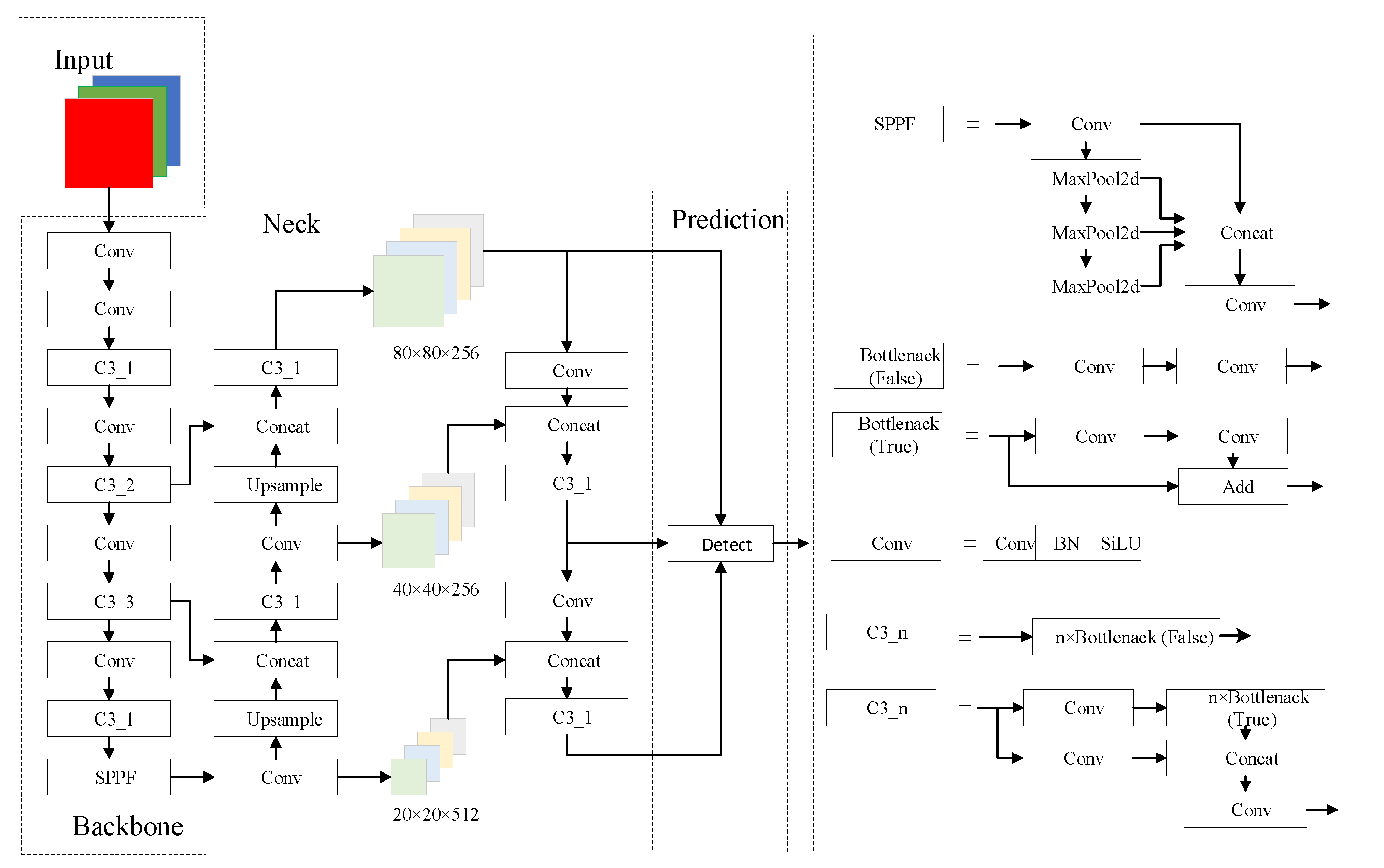
YOLOv5 is a more advanced and popular target detection algorithm, which belongs to a class of YOLO series algorithms. It improves the robustness of the network by using a series of convolutional kernels and feature fusion modules in the feature extraction network and realises an organic combination of data and features in the neck network. YOLOv5s is the smallest and fastest variant of YOLOv5, and in view of the high requirements of distracted driving detection on detection speed, the YOLOv5s network is adopted as the base model. The structure of YOLOv5s is shown in Figure 1.
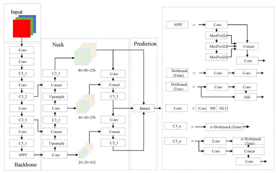
Figure 1.
Structure of YOLOv5s.
YOLOv5s contains four important parts: prediction, neck, backbone and input. The input performs image scaling, adaptive anchor frame computation and mosaic data enhancement to enrich the data volume of the dataset and enhance the performance of the neural network. The backbone focus and CSP (Cross Stage Partial) structures are used to reduce the feature map and extract the corresponding image features. The neck uses an FPN (Feature Pyramid Network) + PAN (Perceptual Adversarial Network) structure to fuse the features extracted by input. The prediction detecting head uses different scales corresponding to the a priori frames to make predictions and classifications.
3. The Algorithm in This Paper
3.1. Overall Network Structure
In order to solve the current distracted driving behaviour detection problems, such as slow recognition speed and low recognition accuracy, and to enhance the recognition performance of the model under the influence of various types of complex environments, based on YOLOv5s, a lightweight model is proposed. The improved model discards the original backbone network and part of the C3 network structure, utilises a combination of Ghostnet and GSConv to realise the lightweight of the model, which greatly reduces the computational and parametric quantities of the model, and enhances the recognition speed of the model; meanwhile, the incorporation of SoftNMS and the CBAMs ensures an improvement in the model’s accuracy. The improved model network structure is shown in Table 1.

Table 1.
Improved network structure of the model.
3.2. Lightweight Model Ghostnet
The Ghostnet lightweight convolutional network focuses its attention on the large number of redundant feature pictures generated after convolution compared to other lightweight networks. In a well-trained deep neural network, a large or even redundant number of feature images are usually included to ensure a comprehensive understanding of the input data. While Ghostnet generates more feature maps using fewer parameters to ensure the richness of the feature maps, Ghostnet builds the Ghost module, which can be utilised to generate a large number of redundant pictures faster with less arithmetic requirements.
The process of extracting target features using the Ghost module is shown in Figure 2 and Figure 3, which are divided into two parts. The first part does the standard convolution operation, using the given size of the convolution kernel to operate on the input image to obtain the feature maps of each channel of the detection target; the second part linearly transforms the feature maps generated in the first part to obtain similar feature maps, which produces a high-dimensional convolution effect and reduces the computational and parametric quantities of the model; finally, the two parts are spliced together to obtain the complete output layer.

Figure 2.
Standard convolution.
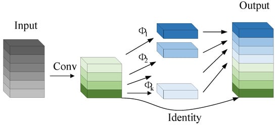
Figure 3.
Ghost module convolution.
For standard convolution, given the input data , where and are the width and height of the input feature map, respectively, and is the amount of channels of the input, the resulting operation for generating an arbitrary convolutional layer of feature maps is shown in Equation (1).
where is the bias term, is the output feature map with output channels and is the convolution kernel of this feature layer. In this convolution process, the number of channels, , and the number of convolution kernels, , can be very large, which makes the computational increase. The formula for is shown in Equation (2).
where is the size of the convolution kernel and and are the width and height of the output feature map, respectively.
The Ghost module performs a convolution operation on a portion of the existing feature maps, which is performed using one standard convolution for original output feature maps, , where . The procedure is shown in Equation (3).
where is the convolution kernel used in this feature layer, omitting the presence of the bias term.
In order to further obtain the required feature maps, a series of simple linear operations are used on the obtained -dimensional feature maps to generate similar feature maps, which is shown in Equation (4).
where is the ith original feature map in is the th linear computation for generating the th similar feature map, . This part of the computational is shown in Equation (5).
where is the average kernel size for each linear operation. The theoretical speedup after using the Ghost module is derived from Equations (2) and (5), as shown in Equation (6).
Since the magnitude of is similar to and , similarly, the parameter compression ratio is approximately equal to , resulting in . By calculation, the overall compression ratio of the model is approximately times.
3.3. Lightweight Convolution Method GSConv
The lightweight convolution GSConv is a new convolution method based on deeply separable convolution (DSC), standard convolution (SC) and channel blending operations; the idea is to separate the input channels into multiple groups, perform an independent depth-wise separable convolution for each group and then recombine them by means of channel blending, the structure of which is shown in Figure 4.
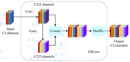
Figure 4.
Structure of GSConv.
When the convolution size , is the size of the output, is the number of input channels and is the number of channels of the output, then the standard convolution, , produces the computation shown in Equation (7).
The computational effort generated by the depth-wise separable convolutional, , is shown in Equation (8).
This results in a compression ratio between the and as shown in Equation (9).
In the GSConv lightweight convolution, each convolution kernel is divided into two parts: the Ghost Convolution Kernel and the Main Convolution Kernel. The Main Convolution Kernel acts as the core bit and performs the main computation, while the Ghost Convolution Kernel is used to complement the computation of the Main Convolution Kernel, thus achieving the effect of grouped convolution and greatly reducing the amount of computation. Its calculation formula is shown in Equation (10).
where denotes the dissimilarity operation, represents the length of the input and denotes the th element of the input, which in a convolution corresponds to the amount of random shifts. The time complexity of GSConv is low due to the fact that it retains the channel-dense convolution, which is shown in Equation (11).
The time complexity formulas for the standard convolution, , and the depth-wise separable convolution, , are shown in Equations (12) and (13).
where is the number of channels in the output and is the number of channels in the convolution kernel. In this convolution operation, the Main Convolution Kernel and the Ghost Convolution Kernel are in different positions horizontally and vertically, and it adopts the strategy of channel mixing and shuffling, grouping the input channels and letting the channels in each group be cross-computed, which enhances the performance of the network and reduces the number of parameters in the model.
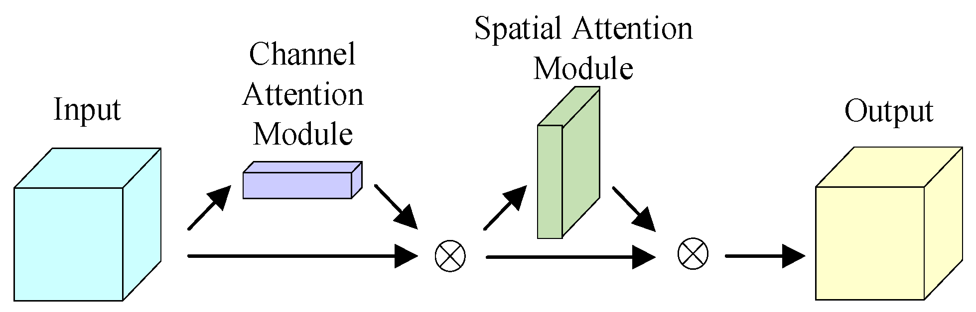
3.4. CBAM
Incorporating the CBAM on the basis of YOLOv5 aims to improve the accuracy of the algorithm by means of feature weighting. The CBAM, as a comprehensive and powerful attention mechanism, takes advantage of its ability to fuse spatial and channel attention, focuses on the spatial and channel regions of some features, and then enriches the feature information by combining the MaxPool operation and the AvgPool operation. The model’s structure is shown in Figure 5.
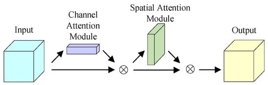
Figure 5.
The structure of the CBAM.
In the CBAM, the input, firstly, passes the channel attention module, which performs an element-by-element multiplication operation between the output one-dimensional convolution of the channel attention and the input, so as to obtain the input enhanced by the channel attention, and then, passes the spatial attention module, which performs an element-by-element multiplication operation between the output two-dimensional convolution of the Spatial Attention and the input feature map of the Module again. The final output feature map of the CBAM is obtained.
The network structure of the channel attention module in the CBAM is shown in Figure 6.
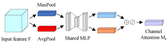
Figure 6.
Channel attention module in the CBAM.
Firstly, the input feature map is passed through the MaxPool and AvgPool layers to aggregate the spatial information of the input feature maps to obtain the MaxPool and AvgPool features, respectively; then, it is passed through a shared network, which consists of a multilayer perceptron (MLP) and a hidden layer, respectively, and then the output features from the shared network are summed element-by-element, and finally a sigmoid activation operation is performed to produce a one-dimensional convolution of the channel attention. The computational procedure of the channel attention module is shown in Equations (14) and (15). denotes the initial input feature map, denotes the generated channel attention one-dimensional convolution, denotes the output feature map after the channel attention convolution, denotes multilayer perceptron, denotes the element-by-element multiplication operation and denotes sigmoid activation function.
The structure of the Spatial Attention Module of the CBAM is shown in Figure 7.
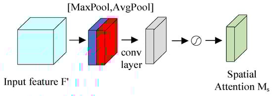
Figure 7.
Spatial attention module in the CBAM.
The input to the spatial attention module is the feature map enhanced by the channel attention module. The feature map is first aggregated by MaxPool and AvgPool to aggregate the channel information of the feature map, thus generating two two-dimensional feature maps, which represent the MaxPool and AvgPool features of the feature map in the channel, respectively; then, the standard convolutional layer is used to perform the connectivity as well as convolutional operations; and finally, the spatial attention two-dimensional convolution is generated by the sigmoid activation function. The computational process of the Spatial Attention Module is shown in Equations (16) and (17). represents the feature map obtained after processing by the channel attention module, denotes the resulting two-dimensional convolution of the spatial attention, denotes the resulting output feature map after the convolution of spatial attention, denotes the element-by-element multiplication operation, denotes the sigmoid activation function and represents the convolution operation with dimensions of .
3.5. The Soft-NMS Algorithm
The main idea of the NMS (non-maximum suppression) mechanism is to sort the anchor frame scores in the score set from highest to lowest, traverse the calculation of the proportion of overlap area between each anchor frame and the highest-scoring candidate frame, and if the calculation result is larger than the threshold, the anchor frame is directly removed. However, this method may lead to the detection failure of the target appearing in the overlapping area; in addition, if the threshold value is taken to be too small, it may cause the neighbouring targets to miss the detection phenomenon, and if the threshold value is too large, it may also lead to a target with multiple detection frames.
In order to avoid missing or re-detection in detecting the target object, the Soft-NMS algorithm is introduced; the core idea of this algorithm is that when the overlap area ratio of two anchor frames is greater than the threshold value, it will not directly return the score to zero but will reduce the score of the anchor frame, and the higher the overlap area ratio is, the more the score will be reduced. Compared with the traditional NMS algorithm, Soft-NMS only needs to make minor changes to the traditional NMS, does not add extra parameters, does not need extra training, is easy to implement, the complexity of the algorithm is the same as that of the traditional NMS, and is highly efficient to use. The flow of the Soft-NMS algorithm is shown in Algorithm 1.
| Algorithm 1: Flow of Soft-NMS algorithm. |
| Inputs: Initial Anchor Frame Set B, Score set S, Overlap Ratio Threshold |
| Output: Updated Anchor Box Set and Score Set |
| while do |
| for |
| end |
| end |
4. Experimental Results and Analysis
4.1. Dataset Production
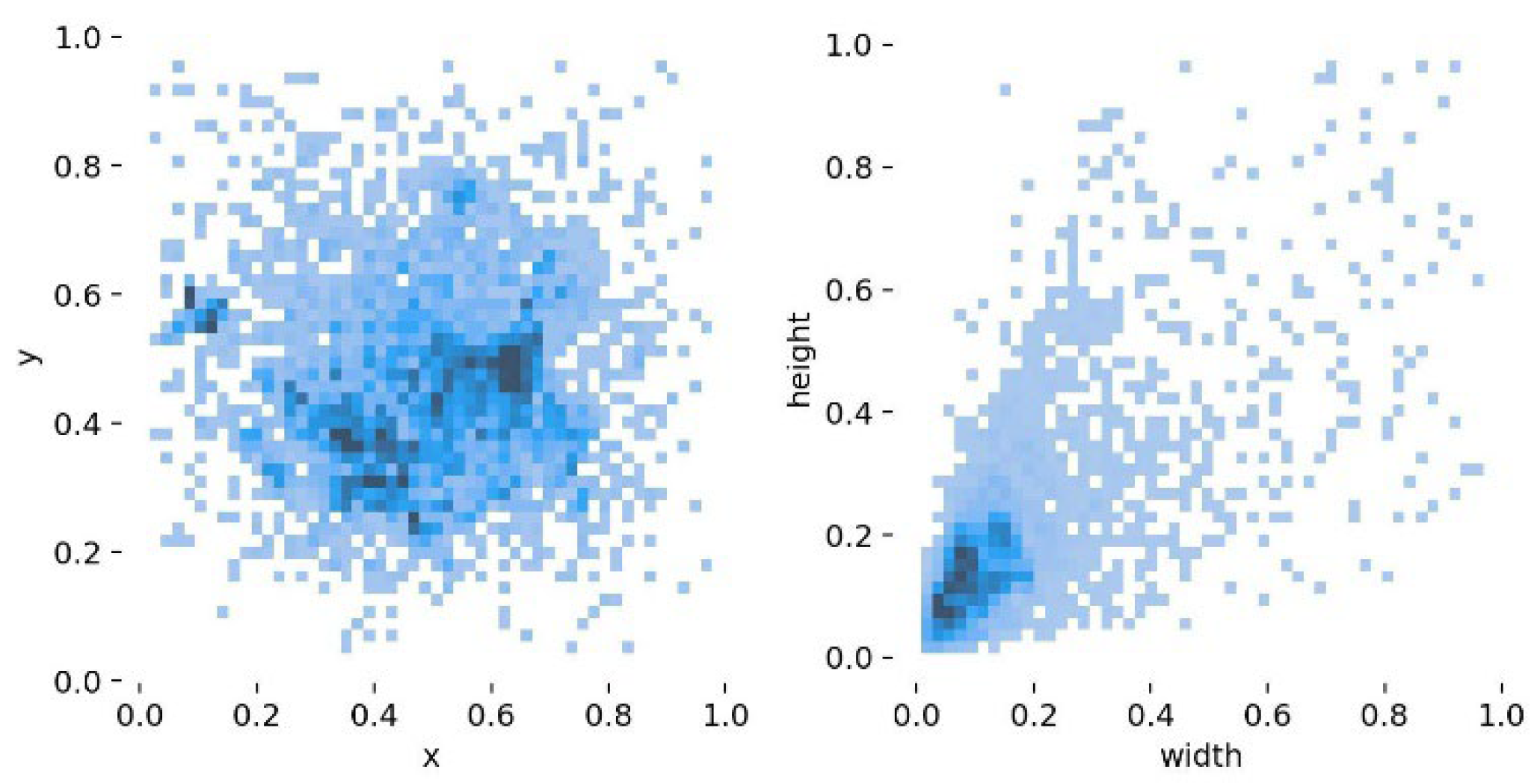
Due to the protection of the privacy of the driver’s driving behaviour, the relevant datasets are almost never made public, and most of the similar datasets are self-made. At present, the most common public dataset is SFD3 (State Farm Distracted Driver Detection), but the data in this dataset have a single orientation, which cannot meet the needs of multi-directional detection of drivers, and it does not detect some special distracted driving behaviours, such as smoking in the process of driving. In this paper, based on the SFD3 dataset, some data captured in different directions and under different conditions are added to enrich the data in the dataset. Then, a labelling annotation tool was used to annotate the target objects one by one, and a total of 8222 image data points were produced. The dataset is randomly divided in the ratio of 7:3, in which there are about 5755 picture data points in the training set and 2467 picture data points in the validation set. The label distribution of the dataset is shown in Figure 8.
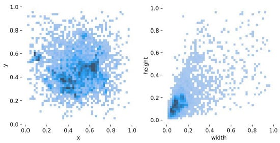
Figure 8.
Distribution of labels in the dataset.
x and y denote the horizontal and vertical coordinates of the centre point of the label box, and the width and height denote the width and height of the label box, respectively. From the data in the figure, it can be seen that the labels are uniformly distributed and belong to multi-scale targets, which are suitable for the detection of distracted driving behaviour by drivers in real-life scenarios.
4.2. Configuration of Parameters and Evaluation of Indicators
In this paper, YOLOv5s is chosen as the base algorithm and is improved based on it. In the experimental environment, NVIDIA RTX 3090 is used for the GPU to satisfy the arithmetic support. The training input image data size is 640 × 640, the batch size is 16, the data enhancement method adopts Mosaic data enhancement, the quantity of workers is set to 12, and the number of epochs is 200.
In this paper, P, R, GFLOPs, parameters and mAP@0.5 are used as the evaluation metrics of model performance. P is the ratio of correct predictions; R is the ratio of selected predictions. The formulas of P and R are shown in Equations (18) and (19).
where, when the IOU threshold is 0.5, TP denotes the quantity of detected frames with the IOU outweighing 0. 5, which is the number of correct detections; FP denotes the number of detected frames with the IOU less than or equal to 0.5, which is the quantity of misdetections; and FN represents the quantity of targets with missed detections. mAP is computed as shown in Equations (20) and (21).
N represents the quantity of categories of target objects, mAP@0.5 denotes the average AP when the IOU threshold is 0.5 and mAP is the area under the P–R curve. mAP@0.5 is often used to reflect the detection ability of the model, which can show the performance of the model well.
4.3. Experimental Results and Analysis
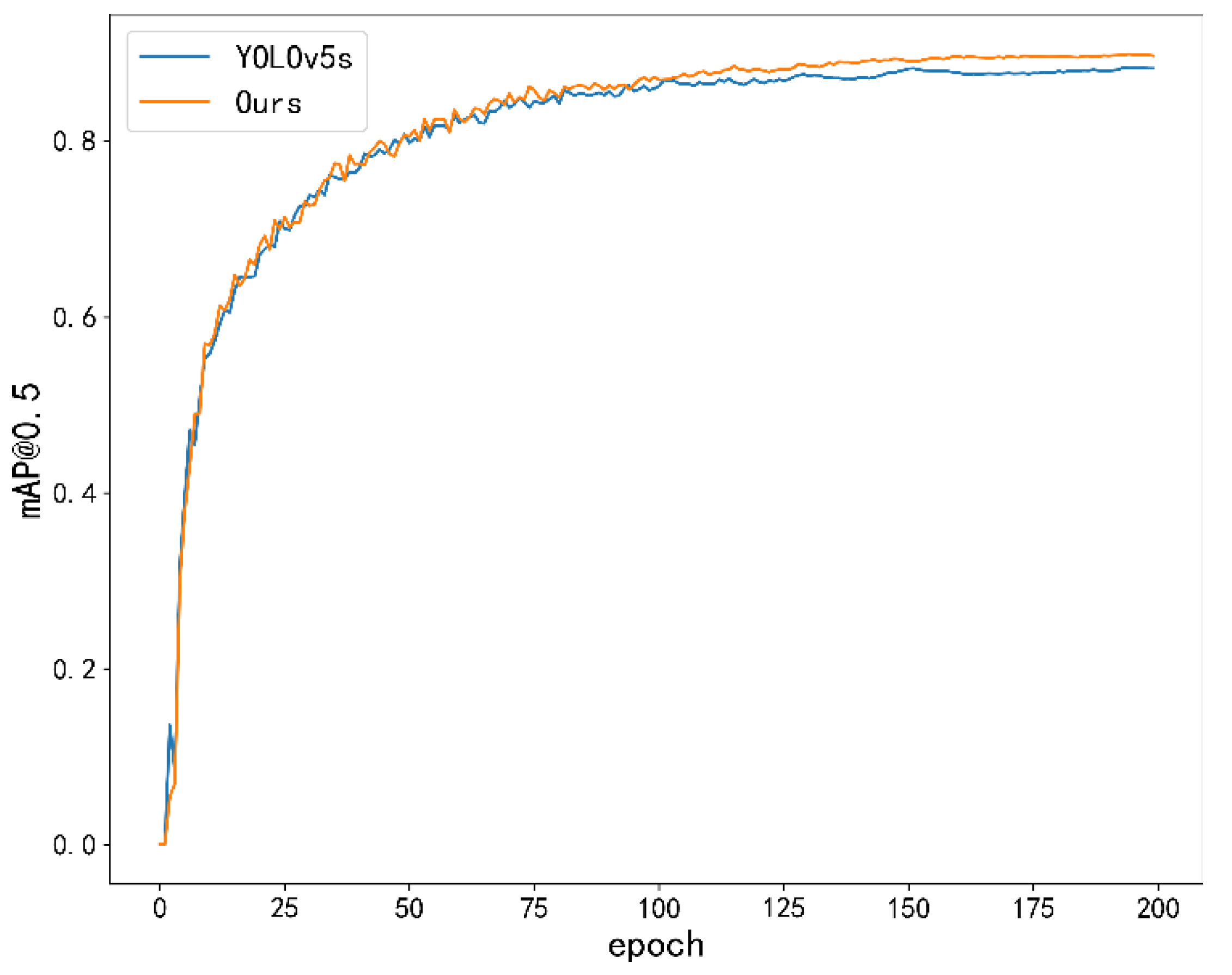
In order to verify the validity of the relevant modules, a number of experiments were carried out on each of the modules to compare their effects on the performance of the original model under the same hardware conditions. The mAP@0.5 comparison between the final model and YOLOv5 is shown in Figure 9.
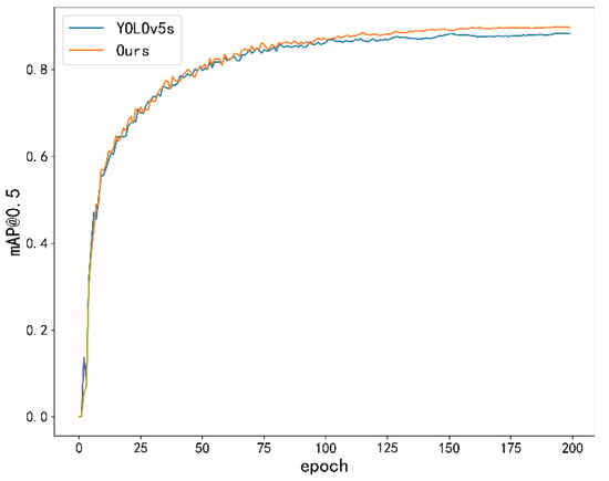
Figure 9.
mAP@0.5 comparison between YOLOv5s and the algorithm in this paper.
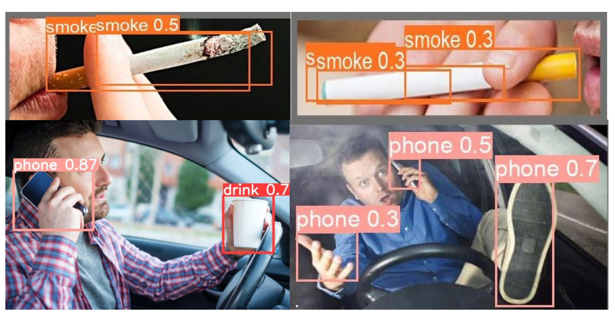
As can be seen from the figure, after a period of training, the improved model has a more obvious improvement in accuracy compared with YOLOv5. While the accuracy is improved, the model also has good performance for phenomena such as error checking and rechecking, as shown in Figure 10 and Figure 11.
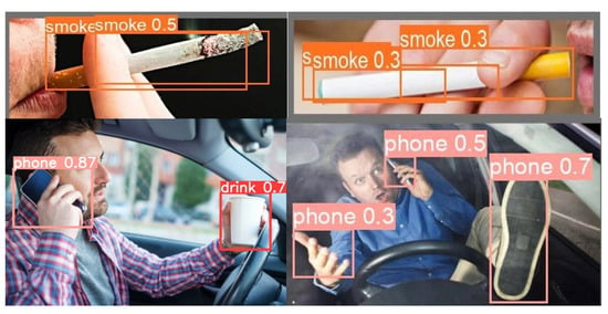
Figure 10.
Original model detection map.
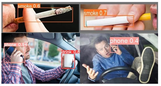
Figure 11.
The detection map of the improved model.
Since the improvement in the accuracy of the improved algorithm depends on the joint action of the modules, it is necessary to verify the role of each module in the model and to calibrate its effectiveness. In this paper, under the same experimental parameters and hardware environment conditions, five sets of ablation experimental results are derived on the homemade dataset, and the experimental results are shown in Table 2 and Table 3.
Table 2.
Results of ablation experiments (1).
Table 3.
Results of ablation experiments (2).
In the table, “√” indicates that the module is introduced and “×” indicates that the module is not introduced. As shown by the results of ablation experiments (a) and (b), Module A, the CBAM, improves the inference time by 1.4 ms, P and R by 2% and 1.9%, respectively, and mAP@0.5 by 0.8% while keeping the Params and GFLOPs almost the same, and the data show that the CBAM reduces the false detection rate to some extent. Module B, Ghostnet, has a relatively good effect on the model, compared with YOLOv5s. Although mAP@0.5 is reduced by 1%, all other data quantities are improved to different degrees, and the reduction in the Params, GFLOPs, and inference makes the model better able to meet the needs of industrialisation. Module C, GSConv, on the other hand, balances the coordination between each of the data, with a good improvement in mAP@0.5 while ensuring that the Params, GFLOPs and inference have been reduced, further meeting the industrialisation requirements. Module D, the SoftNMS algorithm, substantially improves the inference time while keeping the Params and GFLOPs almost the same, reducing the inference by 4 ms compared with YOLOv5s and improving the real-time requirements of the model. Compared with YOLOv5s, the improved model has different degrees of improvement in each data quantity. p and r are improved by 2.6% and 0.1%, respectively; mAP@0.5 is improved by 1.5%; the Params are reduced by 1.6 unit quantities; and the GFLOPs are reduced by 7.6. Clearly, the algorithmic model in this paper has superior performance enhancement in detecting and identifying the distracted driving behaviour of drivers compared with YOLOv5s.
To further validate the superiority of the algorithmic model in this paper, a series of data comparisons with other algorithms of the same type were performed on a home-made dataset. The results of the comparison experiments are shown in Table 4.
Table 4.
Comparison of experimental results.
Compared with YOLOv5s, SSD, YOLOv5x and YOLOv7, the SSD model is faster in operation. mAP@0.5 is able to outperform some of the two-phase detection algorithms, while the SSD model maintains fast operation. However, its Params and ModelSize are a non-negligible influencing factor. The mAP@0.5 improvement in YOLOv5x and YOLOv7 is more obvious, but the growth of its Params and GFLOPs deepens the complexity of the model, and the huge ModelSize of YOLOv5x has a big impact on engineering. The model in this paper has a significant advantage in terms of its Params and GFLOPs. mAP@0.5 has a nice boost and its Inference is not inferior at all. Although ModelSize has a slight increase, it hardly affects the engineering deployment. Therefore, compared with other models, this paper’s model is more suitable for detecting drivers’ distracted driving behaviour.
5. Conclusions
In this paper, based on the traffic safety problems related to driver distracted driving behaviours as the research background, we detect and identify the common distracted driving behaviours produced by drivers in the driving process and propose an improved target recognition algorithm based on the YOLOv5s. The purpose of the algorithm in this paper is to solve the problems of slow recognition, high computation and low recognition accuracy. YOLOv5s is used as the base model, and Ghostnet is used to lighten the model and reduce the computational and parametric quantities of the model. The GSConv module is used to balance accuracy and speed while lightweighting, so that its accuracy will not be drastically reduced. The Soft-NMS algorithm and the CBAM enable the model to have an increase in speed while the accuracy can be improved after lightweighting. The final improved model is compared with the YOLOv5s model. The Params are reduced by about , the GFLOPs are reduced by 7.6 GFLOPs, and mAP@0.5 is improved by 1.5%. In summary, the improved lightweight model provides superior performance in detecting and identifying distracted driving behaviour.
Author Contributions
Writing—original draft preparation, C.L.; writing—review and editing, C.L. and X.N.; supervision, X.N. All authors have read and agreed to the published version of the manuscript.
Funding
This work was supported by a grant from the Hubei Key Laboratory of Intelligent Robot of China (Grant No. HBIRL202009).
Institutional Review Board Statement
Not applicable.
Informed Consent Statement
Not applicable.
Data Availability Statement
The authors can provide the raw data in this work upon reasonable request.
Conflicts of Interest
The authors declare no conflict of interest.
References
- He, K.; Gkioxari, G.; Dollár, P.; Girshick, R. Mask R-CNN. In Proceedings of the IEEE International Conference on Computer Vision, Venice, Italy, 22–29 October 2017; pp. 2961–2969. [Google Scholar]
- Ren, S.; He, K.; Girshick, R.; Sun, J. Faster R-CNN: Towards realtime object detection with region proposal networks. In Proceedings of the 2015 Advances in Neural Information Processing Systems, Montreal, QC, Canada, 7–12 December 2015; pp. 91–99. [Google Scholar]
- Girshick, R. Fast RCNN. In Proceedings of the 2015 IEEE International Conference on Computer Vision, Santiago, Chile, 7–13 December 2015; pp. 1440–1448. [Google Scholar]
- Girshick, R.; Donahue, J.; Darrell, T.; Malik, J. Rich feature hierarchies for accurate object detection and semantic segmentation. In Proceedings of the 2014 IEEE Conference on Computer Vision and Pattern Recognition, Columbus, OH, USA, 23–28 June 2014; pp. 580–587. [Google Scholar]
- Liu, W.; Anguelov, D.; Erhan, D.; Szegedy, C.; Reed, S.; Fu, C.Y.; Berg, A.C. SSD: Single shot multibox detector. In Proceedings of the 2016 European Conference on Computer Vision, Amsterdam, The Netherlands, 11–14 October 2016; pp. 21–37. [Google Scholar]
- Jeong, J.; Park, H.; Kwak, N. Enhancement of SSDby concatenating feature maps for object detection. arXiv 2017, arXiv:1705.09587. [Google Scholar]
- Fu, C.Y.; Liu, W.; Ranga, A.; Tyagi, A.; Berg, A.C. DSSD: Deconvolutional single shot detector. arXiv 2017, arXiv:1701.06659. [Google Scholar]
- Li, Z.; Zhou, F. FSSD: Feature fusion single shot multibox detector. arXiv 2017, arXiv:1712.00960. [Google Scholar]
- Redmon, J.; Divvala, S.; Girshick, R.; Farhadi, A. You only look once: Unified, realtime object detection. In Proceedings of the IEEE Conference on Computer Vision and Pattern Recognition, Las Vegas, NV, USA, 27–30 June 2016; pp. 779–788. [Google Scholar]
- Redmon, J.; Farhadi, A. Yolo9000: Better, faster, stronger. In Proceedings of the IEEE Conference on Computer Vision and Pattern Recognition, Honolulu, HI, USA, 21–26 July 2017; pp. 7263–7271. [Google Scholar]
- Redmon, J.; Farhadi, A. YOLOv3: Anincremental improvement. arXiv 2018, arXiv:1804.02767. [Google Scholar]
- Bochkovskiy, A.; Wang, C.Y.; Liao, H.Y.M. YOLOv4: Optimal speed and accuracy of object detection. arXiv 2020, arXiv:2004.10934. [Google Scholar]
- Vosugh, N.; Bahmani, Z.; Mohammadian, A. Distracted driving recognition based on functional connectivity analysis between physiological signals and perinasal perspiration index. Expert Syst. Appl. 2023, 231, 120707. [Google Scholar] [CrossRef]
- Luo, G.; Xiao, W.; Chen, X.; Tao, J.; Zhang, C. Distracted driving behaviour recognition based on transfer learning and model fusion. Int. J. Wirel. Mob. Comput. 2023, 24, 159–168. [Google Scholar] [CrossRef]
- Ping, P.; Huang, C.; Ding, W.; Liu, Y.; Chiyomi, M.; Kazuya, T. Distracted driving detection based on the fusion of deep learning and causal reasoning. Inf. Fusion 2023, 89, 121–142. [Google Scholar] [CrossRef]
- Lin, Y.; Cao, D.; Fu, Z.; Huang, Y.; Song, Y. A Lightweight Attention-Based Network towards Distracted Driving Behavior Recognition. Appl. Sci. 2022, 12, 4191. [Google Scholar] [CrossRef]
- Zhao, X.; Li, C.; Fu, R.; Ge, Z.; Wang, C. Real-time detection of distracted driving behaviour based on deep convolution-Tokens dimensionality reduction optimized visual transformer. Automot. Eng. 2023, 45, 974–988+1009. [Google Scholar] [CrossRef]
- Cao, L.; Yang, S.; Ai, C.; Yan, J.; Li, X. Deep learning based distracted driving behaviour detection method. Automot. Technol. 2023, 06, 49–54. [Google Scholar] [CrossRef]
- Zhang, B.; Fu, J.; Xia, J. A training method for distracted driving behaviour recognition model based on class spacing optimization. Automot. Eng. 2022, 44, 225–232. [Google Scholar] [CrossRef]
- Feng, T.; Wei, L.; Wenjuan, E.; Zhao, P.; Li, Z.; Ji, Y. A distracted driving discrimination method based on the facial feature triangle and bayesian network. Balt. J. Road Bridge Eng. 2023, 18, 50–77. [Google Scholar] [CrossRef]
- Chen, D.; Wang, Z.; Wang, J.; Shi, L.; Zhang, M.; Zhou, Y. Detection of distracted driving via edge artificial intelligence. Comput. Electr. Eng. 2023, 111, 108951. [Google Scholar] [CrossRef]
- Lu, M.; Hu, Y.; Lu, X. Pose-guided model for driving behavior recognition using keypoint action learning. Signal Process. Image Commun. 2022, 100, 116513. [Google Scholar] [CrossRef]
- Dehzangi, O.; Sahu, V.; Rajendra, V.; Taherisadr, M. GSR-based distracted driving identification using discrete & continuous decomposition and wavelet packet transform. Smart Health 2019, 14, 100085. [Google Scholar]
- Omerustaoglu, F.; Sakar, C.O.; Kar, G. Distracted driver detection by combining in-vehicle and image data using deep learning. Appl. Soft Comput. 2020, 96, 106657. [Google Scholar] [CrossRef]
- Zhao, L.; Yang, F.; Bu, L.; Han, S.; Zhang, G.; Luo, Y. Driver behavior detection via adaptive spatial attention mechanism. Adv. Eng. Inform. 2021, 48, 101280. [Google Scholar] [CrossRef]
- Hossain, M.U.; Rahman, M.A.; Islam, M.M.; Akhter, A.; Uddin, M.A.; Paul, B.K. Automatic driver distraction detection using deep convolutional neural networks. Intell. Syst. Appl. 2022, 14, 200075. [Google Scholar] [CrossRef]
- Zhang, Y.; Chen, Y.; Gao, C. Deep unsupervised multi-modal fusion network for detecting driver distraction. Neurocomputing 2021, 421, 26–38. [Google Scholar] [CrossRef]
- Singh, H.; Sidhu, J. Smart Detection System for Driver Distraction: Enhanced Support Vector Machine classifier using Analytical Hierarchy Process technique. Procedia Comput. Sci. 2023, 218, 1650–1659. [Google Scholar] [CrossRef]
- Aljohani, A.A. Real-time driver distraction recognition: A hybrid genetic deep network based approach. Alex. Eng. J. 2023, 66, 377–389. [Google Scholar] [CrossRef]
- Xiao, W.; Liu, H.; Ma, Z.; Chen, W. Attention-based deep neural network for driver behavior recognition. Future Gener. Comput. Syst. 2022, 132, 152–161. [Google Scholar] [CrossRef]
- Lu, M.; Hu, Y.; Lu, X. Dilated Light-Head R-CNN using tri-center loss for driving behavior recognition. Image Vis. Comput. 2019, 90, 103800. [Google Scholar] [CrossRef]
- Cammarata, A.; Sinatra, R.; Maddio, P.D. Interface reduction in flexible multibody systems using the Floating Frame of Reference Formulation. J. Sound Vib. 2022, 523, 116720. [Google Scholar] [CrossRef]


Disclaimer/Publisher’s Note: The statements, opinions and data contained in all publications are solely those of the individual author(s) and contributor(s) and not of MDPI and/or the editor(s). MDPI and/or the editor(s) disclaim responsibility for any injury to people or property resulting from any ideas, methods, instructions or products referred to in the content. |
© 2023 by the authors. Licensee MDPI, Basel, Switzerland. This article is an open access article distributed under the terms and conditions of the Creative Commons Attribution (CC BY) license (https://creativecommons.org/licenses/by/4.0/).