2.2. The Framework of CrossTLNet
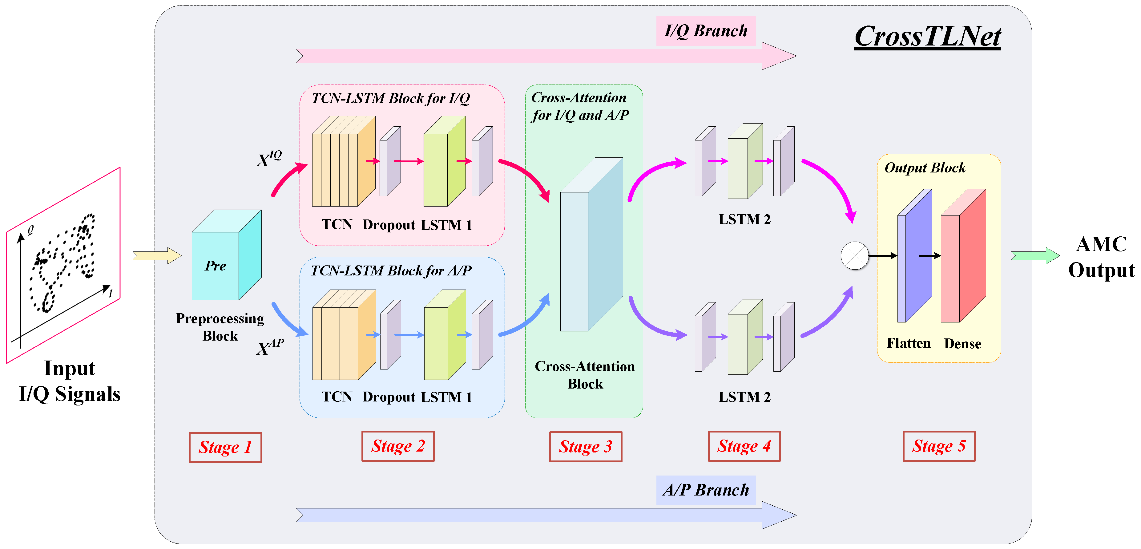
Noticing that the signal, in addition to the commonly used I/Q form, also exhibits distinct features in the amplitude and phase dimensions, i.e., A/P form. Inspired by this, a multi-task learning framework model is proposed, as shown in
Figure 2, named CrossTLNet, which achieves complementary features of I/Q and A/P form.
First, CrossTLNet takes the I/Q signal as its input. After passing through the pre-processing block, the signal is transformed into both I/Q form itself and A/P form, which are separately learned as two tasks. For each task, a feature extraction method with TCN–LSTM is designed to handle long-term dependency features among high-order modulations. Subsequently, a cross-attention method that enables feature interaction between the two tasks is introduced. The interacted signals are then further abstracted through a layer of LSTM, fused into one branch via an outer product operation, and finally classified through a dense layer for AMC.
Specifically, the proposed model consists of five stages.
Stage 1: The pre-processing block takes
I/Q signal as model’s input and transforms it into two parts: the original I/Q signal and the A/P signal for further processing. The transformation to obtain the A/P signal can be denoted as follows:
Stage 2: A symmetric multi-task learning architecture with two TCN–LSTM blocks is designed for the initial extraction of signal features. Each TCN–LSTM block consists of a TCN module and an LSTM module, both with 256 units. The convolutional kernel size is 3, and a dropout layer (dropout rate is 0.5) is inserted after them to prevent overfitting. By combining the TCN module and LSTM module, CrossTLNet becomes more sensitive to features at different time scales, which is beneficial for distinguishing between highly similar high-order modulations. The signal processed by the TCN–LSTM block is then propagated backward in a size of .
Stage 3: The cross-attention block takes the extracted I/Q and A/P signal features from the TCN–LSTM blocks. Through a process of interaction, one task branch of the model could learn features in the other form of the signal, enhancing its focus on important features. The signal after the cross-attention block maintains the same dimensions and continues to propagate backward.
Stage 4: The signal after passing through the cross-attention block undergoes further feature extraction through a new LSTM layer with 128 units. To prevent overfitting, dropout layers (dropout rate is 0.5) are added before and after the LSTM layer. The output is a one-dimensional feature sequence of 128 bits.
Stage 5: The I/Q and A/P signals after
Stage 4 are fused through an outer product operation and finally fed into the output block. Mathematically, this can be represented as:
where
represents all operations from
Stage 1 to
Stage 4, and
represents the input to the flatten layer. The size of
is
. After the outer product operation, the data features from the two branches are adequately amplified and fused. Following the flatten layer, the final classification is performed by the dense layer, resulting in the output of the results.
The following will provide specific details about the method with TCN–LSTM for high-order modulations and the method of cross-attention.
2.3. The Method with TCN–LSTM for High-Order Modulations
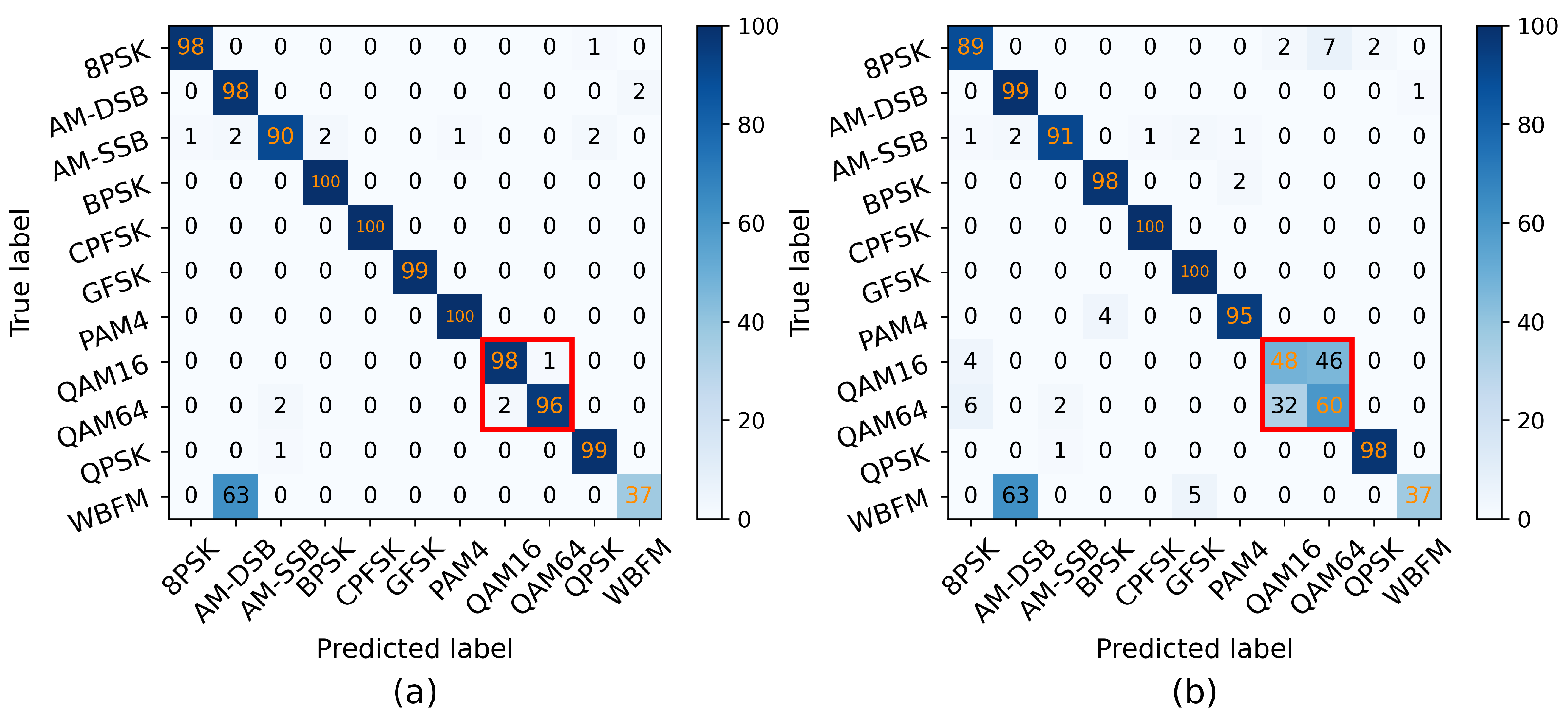
Previous studies have encountered the issue of classification confusion when dealing with high-order modulations. Compared with conventional DL methods such as CNN, a method with TCN–LSTM is proposed for different high-order modulations, which achieves accurate classification by improving the model’s capability to capture long-term dependency features. Without loss of generality, two different high-order modulations of the same scheme HMOD are denoted as HMOD-A and HMOD-B, respectively, where HMOD-B is of higher order than HMOD-A, i.e., . In this way, HMOD-A and HMOD-B are used as examples to elucidate the motivation and the design details of the suggested method.
An analysis is conducted first to understand the reasons behind the classification confusion between HMOD-A and HMOD-B. In an ideal scenario, HMOD-A and HMOD-B utilize A and B distinct symbols, respectively, for information representation. They possess noticeable differences, and there are clear distinctions in their amplitude and phase representations as well. However, since both of them are based on the same HMOD constellation distribution, if a DL model only focuses on capturing and learning local features, it may find the two very similar and thus easily confuse them.
Drawing from the above analysis, it becomes evident that for a DL model to accurately differentiate between
HMOD-A and
HMOD-B, it must possess the capability to focus on capturing global features. Compared to CNN, TCN excels at capturing global features, enabling a more comprehensive distinction between the features of
HMOD-A and
HMOD-B. Inspired by [
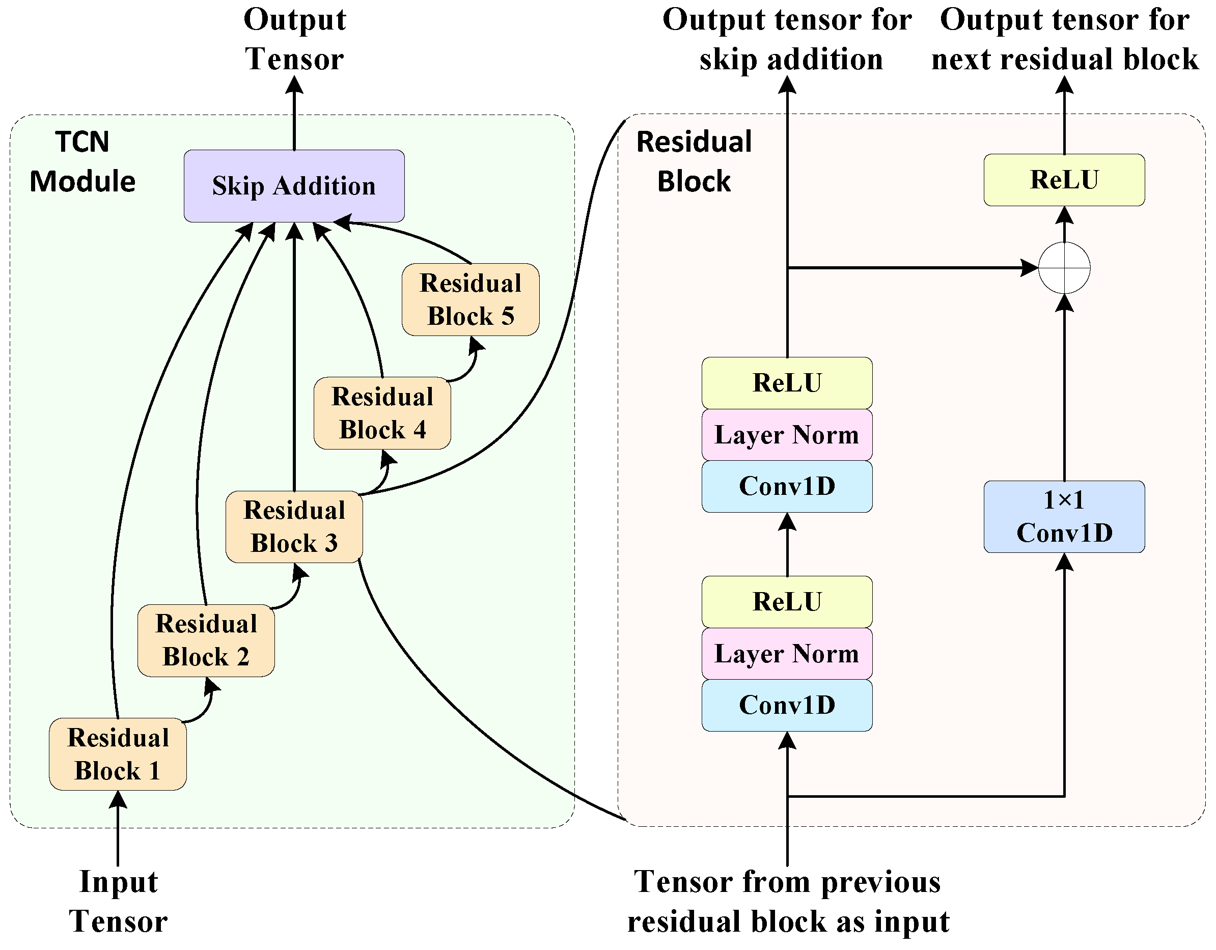
10], the TCN module in TCN–LSTM block is designed as illustrated in
Figure 3. The TCN module consists of five residual blocks. Drawing inspiration from DenseNet, skip connections are also employed between each residual block to enhance the gradient flow. Within each residual block, one-dimensional causal convolutions are utilized. Unlike traditional convolutions, causal convolutions cannot see future data. In other words, the output at time
t is contingent solely upon the input at or before time
t in the preceding layers, imposing a strict temporal constraint. This enables TCN to effectively handle time series data. Moreover, dilated convolutions with dilation factors of 1, 2, 4, 8, 16, and 32 are also applied in the one-dimensional causal convolution. This allows TCN to exponentially increase its receptive field without incurring pooling-related information loss, enabling each convolutional output to encompass a larger range of information. This equips TCN with robust long-term features processing capabilities and the capacity to capture global features. Following the one-dimensional convolution, layer normalization is employed to enhance the stability of model training. Furthermore, for other high-order modulations, effective classification can be achieved by adjusting the number of residual blocks in the TCN module and units in the one-dimensional convolution.
While LSTM can also address the issue of long-term dependencies in time series data, TCN has an advantage over LSTM in processing sequences due to its parallel computation capability. TCN can process the entire sequence simultaneously, whereas LSTM needs to handle each time step sequentially. This means that TCN can more effectively capture spectral features in the signal without being limited by the sequence length. In comparison, HMOD-B signals are more complex and have more spectral features compared to HMOD-A. Therefore, better parallelism is needed to capture these features. Additionally, considering that LSTM uses gating mechanisms to control information flow for handling long-term dependencies, improper settings of these gating mechanisms can lead to issues like information flow obstruction or gradient vanishing, potentially causing the forgetting of important information. TCN, on the other hand, does not have gating mechanisms, allowing it to more stably and effectively capture long-term features between HMOD-A and HMOD-B.
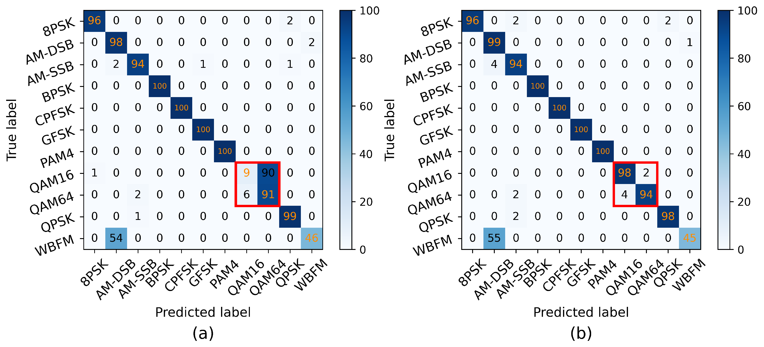
In CrossTLNet, inspired by the hybrid structure of CNN–LSTM, we combine the designed TCN module with the LSTM module to form TCN–LSTM block. This combination not only mitigates the gradient vanishing problem in LSTM but also enhances the model’s ability to extract and represent signal features. In fact, this structure achieves better performance than using TCN alone. In the ablation studies of
Section 3, the impact brought by the TCN module will be further validated.
2.4. The Method of Cross-Attention
I/Q and A/P signals possess distinct dimensional features. Inspired by multi-modal data fusion, a cross-attention method is innovatively introduced, as illustrated in
Figure 4, to enable interaction and emphasize the unique features from both I/Q and A/P.
Unlike the conventional attention mechanism, the query matrix , the key matrix , and the value matrix for each task branch are separately calculated, and and are shared, denoted as the matrix . Next, the similarity matrix for matrix of I/Q task branch and of A/P task branch is calculated, and the Softmax function is utilized to calculate attention weights along the A/P dimension and along the I/Q dimension of , respectively. Subsequently, the pairs and are cross-multiplied, and then passed through a dense layer, respectively. Finally, the cross-attention for the I/Q task branch is obtained, denoted as , and for the A/P task branch, denoted as .
Mathematically, it can be expressed as:
where
represents the dimension of the matrix
, playing a role in scaling the dot product to mitigate the vanishing gradient issue associated with the Softmax function [
11].
represents the operation of passing through a dense layer. The dense layer serves to align dimensions and facilitate further processing. The interaction of I/Q and A/P data through cross-attention incorporates features from the other dimension, which has a positive impact on the final classification accuracy. The results of the ablation studies in
Section 3 also demonstrate this.
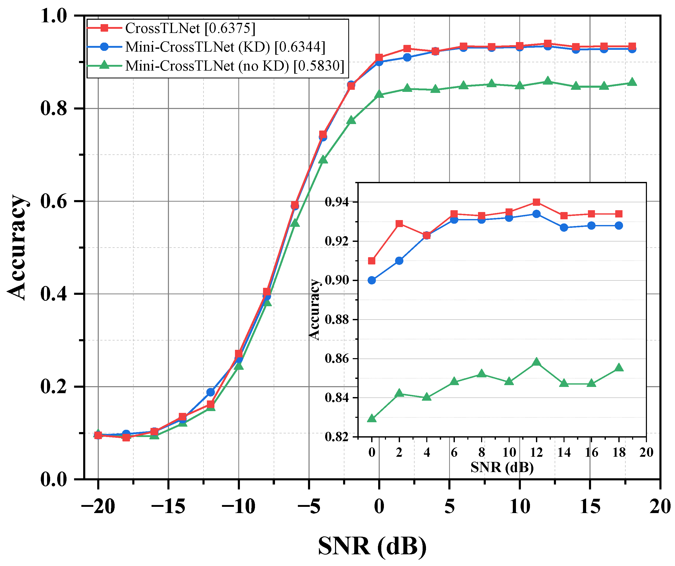
2.5. The Method of Model Lightweighting
In resource-limited scenarios, deploying smaller models is necessary, which is often overlooked by many researchers. Therefore, a simple and effective model lightweighting method is designed with knowledge distillation [
12]. In essence, knowledge distillation involves transferring the knowledge learned by a teacher model (which is large) through the training process to a student model (which is small), enabling the smaller model to possess the generalization capabilities of the larger one. The lightweighting method combines feature-based knowledge distillation and logits-based knowledge distillation. This design greatly facilitates the student model in learning different layers’ responses of the teacher model, enhancing distillation accuracy, while achieving a higher model compression rate.
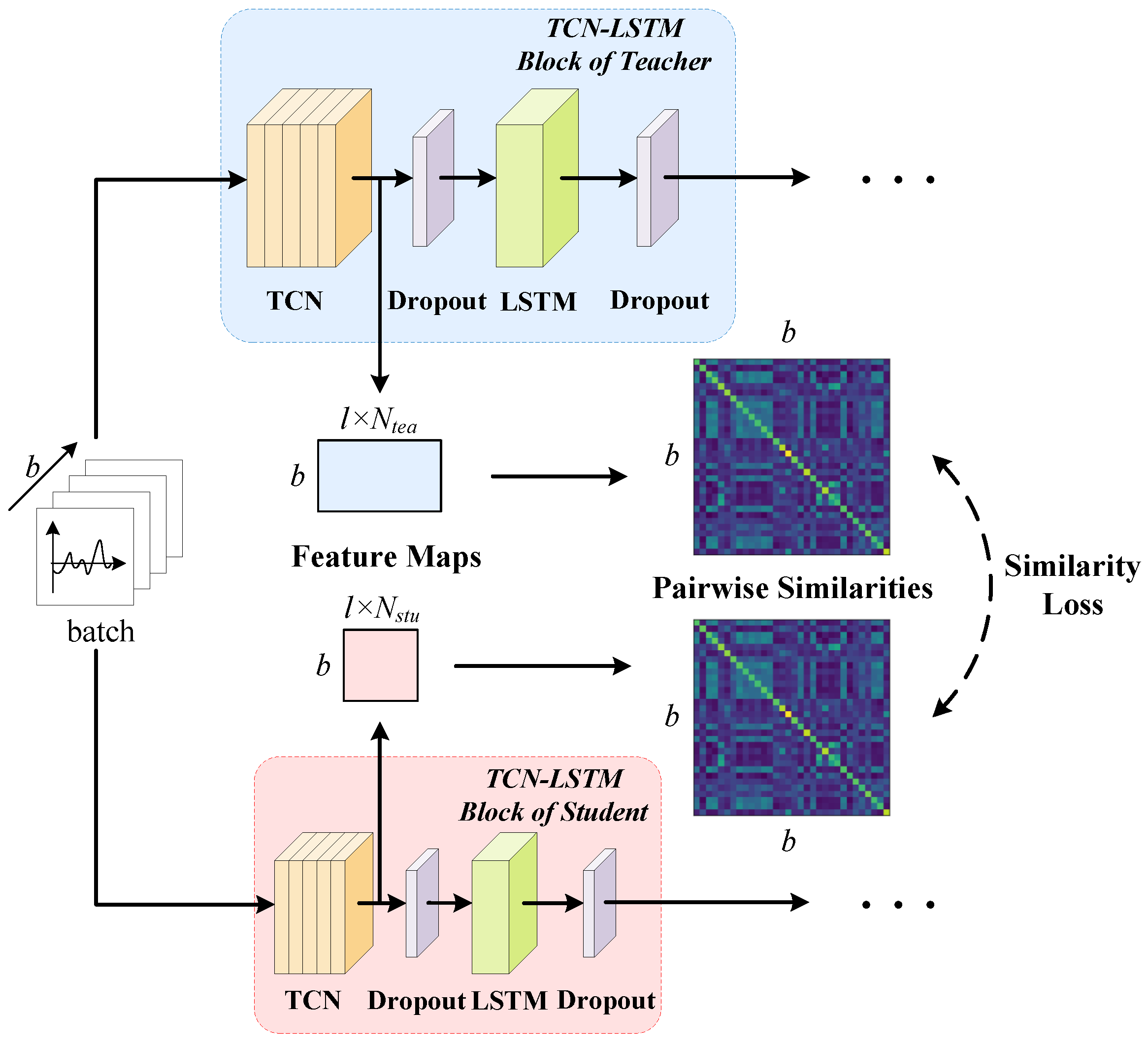
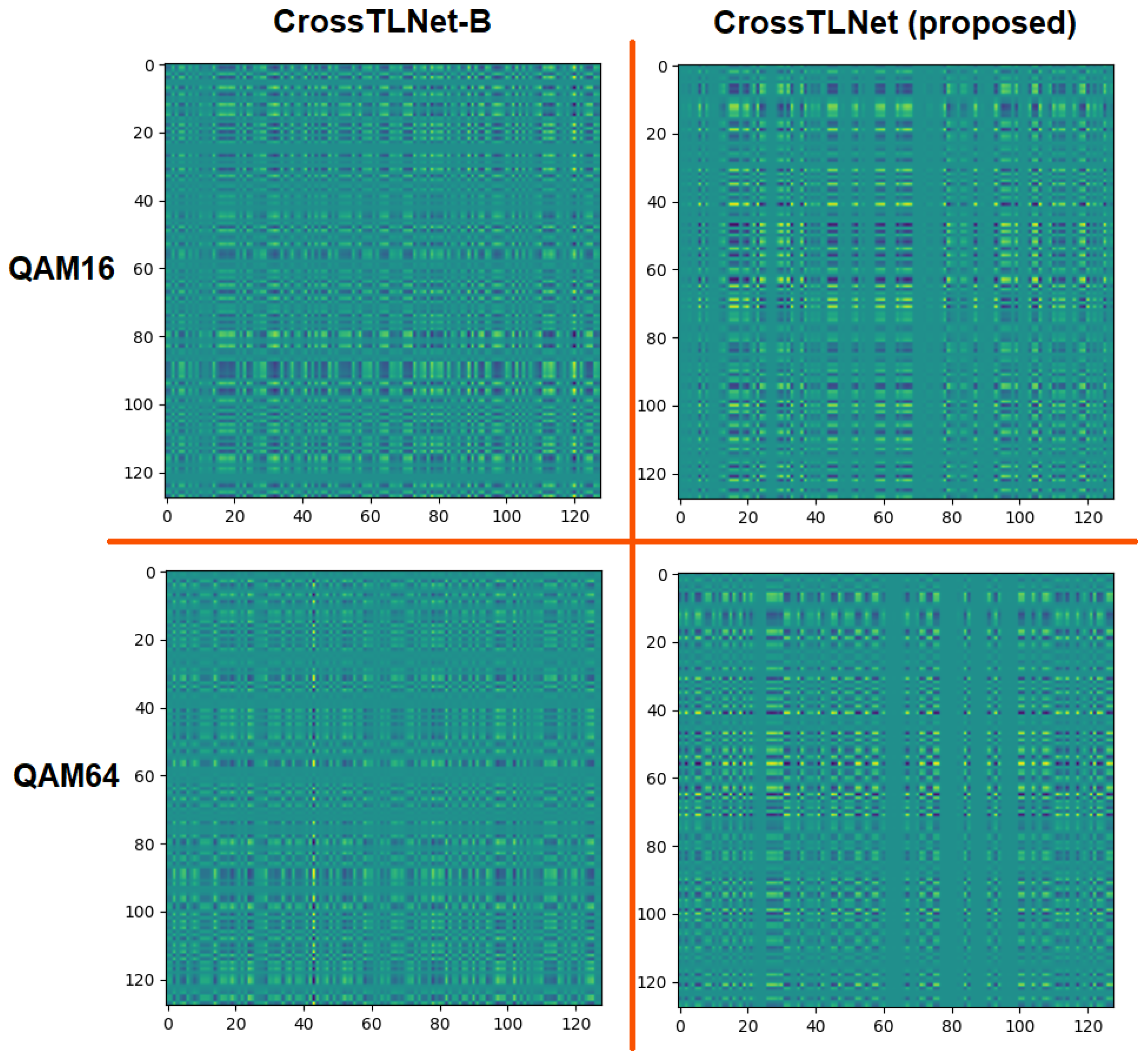
For both the student and teacher models, if the student model can learn not only the output results of the teacher model but also its way of thinking (that is, the responses of the intermediate layers), it will be more advantageous for enhancing the effectiveness of knowledge distillation. The intermediate feature responses of an excellent student model must be similar to those of the teacher model. Inspired by [
13], we output the feature maps after the TCN module in CrossTLNet (both I/Q and A/P branches) and minimize their difference between the student and teacher during the distillation process, as shown in
Figure 5.
For a batch of input with a batch-size of
b, after passing through the TCN module, the teacher and student models obtain feature maps of size
and
, respectively, denoted as
and
. Here,
l represents the sampling length of the input signal, and
and
represent the number of units in the TCN module for the teacher and student models, respectively. Subsequently, in order to align the dimensions of the feature maps, the feature maps are multiplied with their transpose to obtain feature maps of size
for both the teacher and student models. To reduce the numerical range and stabilize the model training, L2 normalization is applied to the transformed feature maps, and the results are denoted as
and
for the teacher and student models, respectively. Therefore, the objective of feature-based knowledge distillation is to minimize the difference between the feature maps, which is denoted as the similarity loss
. Mathematically,
where
represents the L2 norm. Therefore, the similarity loss
can be defined as:
where
represents the Frobenius norm. The two terms on the right-hand side of Equation (
7) represent the similarity losses after the TCN modules for the I/Q branch and the A/P branch, respectively.
The reference [
14] points out that the vanilla knowledge distillation with KL divergence requires an exact match of logits outputs between the teacher and student models, which is too strict. In fact, it is only necessary to ensure that the relative ranks of logits between the student and teacher are consistent, and the specific numerical values are not of concern. Inspired by this, compared to the classic KL divergence, we prefer to use the Pearson’s distance
to measure the logits outputs of the teacher and student models. Denote the logits outputs of the student and teacher models as
and
, respectively, then:
where
T is the temperature coefficient, higher temperature value results in a softer probability distribution across different classes.
and
represent the softened probability distributions after temperature scaling. “
” indicates that the
is computed along the rows.
represents the Pearson correlation coefficient,
represents covariance, and
represents standard deviation, respectively.
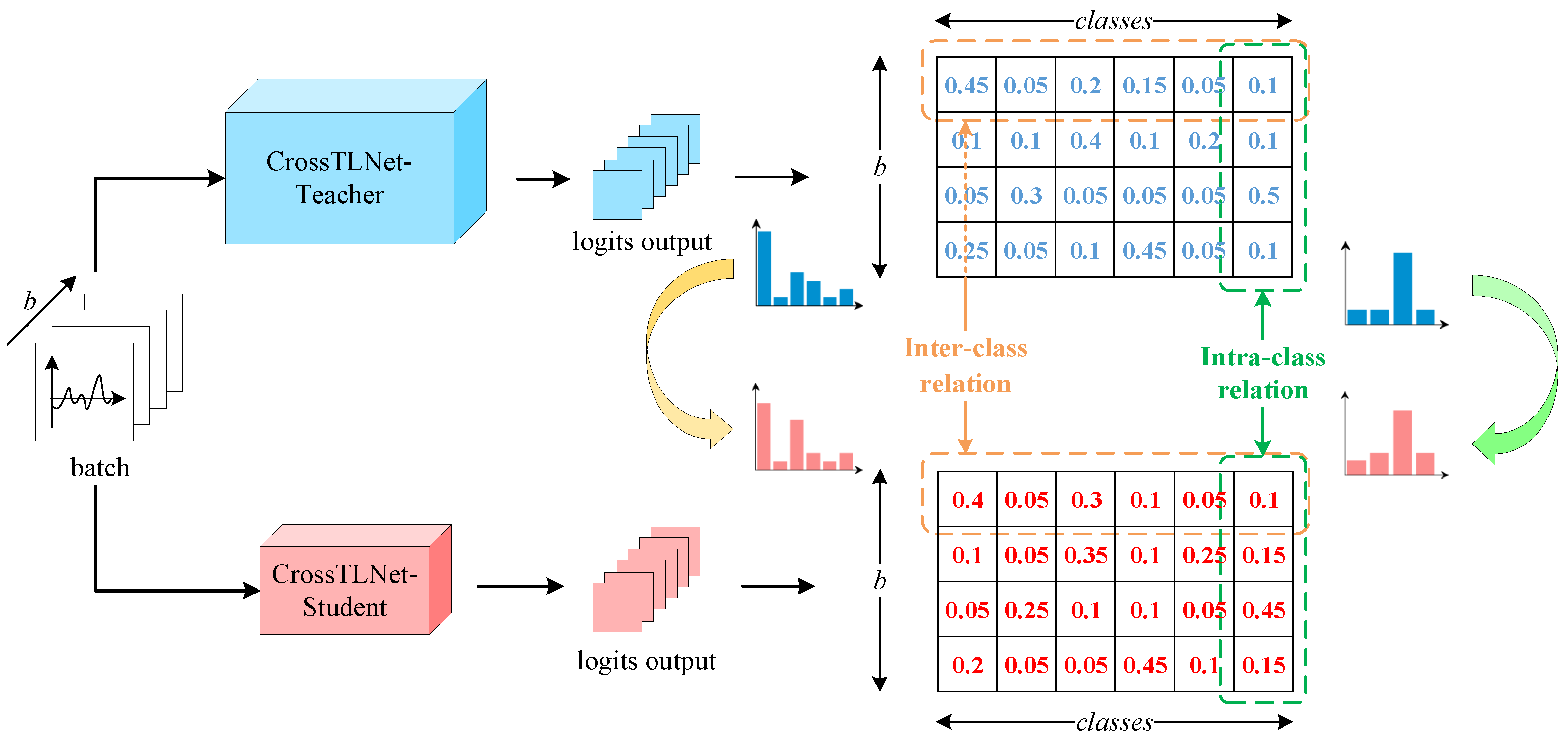
For a batch of input with a batch-size of
b and
c classes, the model’s logits output is a
matrix. Each row reflects the inter-class relation between different classes, while each column reflects the intra-class relation of the same class in a batch. In the case of logits-based knowledge distillation, the objective is to ensure that the teacher and student models exhibit comparable relative ranks in the inter-class and intra-class relation in the logits matrix, as illustrated in
Figure 6.
Mathematically, we can represent the logits loss
as:
where
represents the inter-class loss,
represents the intra-class loss, and the notations “
” and “
” represent row-wise and column-wise calculations, respectively.
In summary, the overall training loss
can be composed of three parts: the original classification loss
, the feature-based loss
, and the logits-based loss
, which can be defined as:
where
,
, and
are weighting factors. In this way, we can utilize the total loss
for knowledge distillation to lightweight the proposed CrossTLNet. The principle of Occam’s Razor suggests that the simplest explanation is often the best. Therefore, compared to many sophisticated knowledge distillation methods, our method is quite straightforward and simple. This means it is easier to implement in practice, which is beneficial for the actual application and deployment of CrossTLNet.


