Model Reference Adaptive Observer for Permanent Magnet Synchronous Motors Based on Improved Linear Dead-Time Compensation

Abstract

Aiming at the problem that the model reference adaptive observer (MRAS) is sensitive to the parameters of the motor model, this paper designs a model reference adaptive observer with resistance adaption and considers the influence of the inverter dead zone. The method introduces the online identification of resistance on the traditional reference adaptive observer model, corrects the resistance parameters of the model’s reference adaptive observer in real time, selects PI as the adaptive law, and proves the stability of the adaptive law using Popov’s stability theorem. To study the influence of the inverter dead zone on the voltage parameters in the estimation model at low speeds, an improved linear dead zone compensation method is proposed to improve the model reference adaptive observer, which eliminates the voltage error between the estimated motor model and the actual motor model. For a given rotational speed of 300 rpm, the observed errors of sliding mode observer (SMO) and traditional MRAS in a steady state were 8.3% and 6%, respectively, and the rotational speed error was controlled to 1.6% using the compensation scheme proposed in this paper. After compensation, the resistance identification error was reduced from 17% to 1.6%. The simulation and experimental results showed that the accuracy of position estimation can be significantly improved using dead zone compensation under low-speed conditions, and the dead zone compensation can improve the accuracy of the online recognition of the resistance.

1. Introduction

Permanent magnet synchronous motors (PMSMs) are widely used in many fields such as automotive, medical, and new energy because of their many advantages, such as a high power density, high efficiency, and a high torque-to-volume ratio. The commonly used magnetic field orientation control FOC requires accurate position information [1]. The position information can be obtained by position or speed sensors, but the installation of sensors increases the size and cost of the motor. The sensors cannot be installed in some specific occasions, so the realization of the accurate estimation of the rotor position of the motor under conditions where there are no sensors is a major focus of the current permanent magnet synchronous motor control research. Model reference adaptive systems (MRASs) have become a commonly used sensorless control method due to their robustness, fast dynamic response, and a simple and easy to implement algorithm [2]. However, the estimation of rotational speed by MRAS depends on the motor parameters, resistance, and other parameters of the motor which change in real time during the actual operation. For this problem, domestic and foreign experts have proposed some solutions. Aiming at addressing the shortcomings of weak robustness and poor anti-interference ability of the traditional PI controller, Refs. [3,4] combine a fuzzy controller with an MRAS and verify that it can improve the dynamic performance and anti-interference ability of the system.

Resistance is a temperature-sensitive parameter, and most of non-inductive controls use the resistance parameter when the motor is designed or measured offline. When the temperature of the environment in which the motor is located changes or the motor output torque increases and the temperature rises, the accuracy of the non-inductive control (e.g., rotational speed, position) and the efficiency of the motor are reduced due to the change in the actual value of the resistance. Therefore, real-time identification of the resistance is necessary in the process of motor operation, and Refs. [5,6,7,8,9,10] performed online identification of the resistance based on MRAS observations of rotational speed, which effectively improved the accuracy of the observer. Therefore, it is necessary to recognize the resistance in real time during the operation of the motor. Ref. [11] utilized an Extended Kalman Filter (EKF) to identify the rotor magnetic chain, the basis of MRAS speed observations. Limited by the rank of the motor equation of state, it is not possible to identify the resistance, inductance, and magnetic chain parameters simultaneously based on the observation of the rotational speed. Therefore, Ref. [12] adopts a step-by-step estimation of the resistance and magnetic chain to further improve the performance of the MRAS. During the low-speed operation of the motor, the turn-on time of the inverter power tubes was shorter, and was greatly affected by the dead time. The nonlinearity of the inverter will have an impact on the rotor position observation as well as online identification of the resistance. Ref. [13] added dead time compensation into the MRAS observer, improving the accuracy of the position estimation and the efficiency of the motor operation. Considering the effect of the actual sampling frequency, Ref. [14] used the discrete model of the system as an adaptive model to estimate the stator current. The optimized gradient descent method served as an adaptive rate to estimate the rotational speed, improving the accuracy of the rotational speed estimation. Ref. [15] proposed an online estimation strategy of magnetizing inductance based on the inverse potential model with reference to the MRAS and the Second-Order Sliding Hyper-Twisting Algorithm (STA). Compared with the traditional flux-based MRAS identification strategy, it does not have pure integral and differential operations in both the reference and adaptive models. It can solve the problems of the integral priming, dc bias, and high-frequency noise amplification. However, these schemes are not satisfactory for MRAS observations at low speeds with loads.

In this study, the MRAS observer based on online resistance identification was used to observe the position and speed information, and the PI controller was selected. The PI controller was used to observe the position and speed information based on the online resistance recognition MRAS observer. An improved dead zone compensation method was used to implement a linear dead zone compensation scheme with variable gain according to the sampled current, which effectively avoids mis-compensation due to errors in judging the polarity of the current. The simulations and experiments proved that the proposed scheme can operate MRAS-based sensorless motor control more effectively under loading and low-speed conditions.

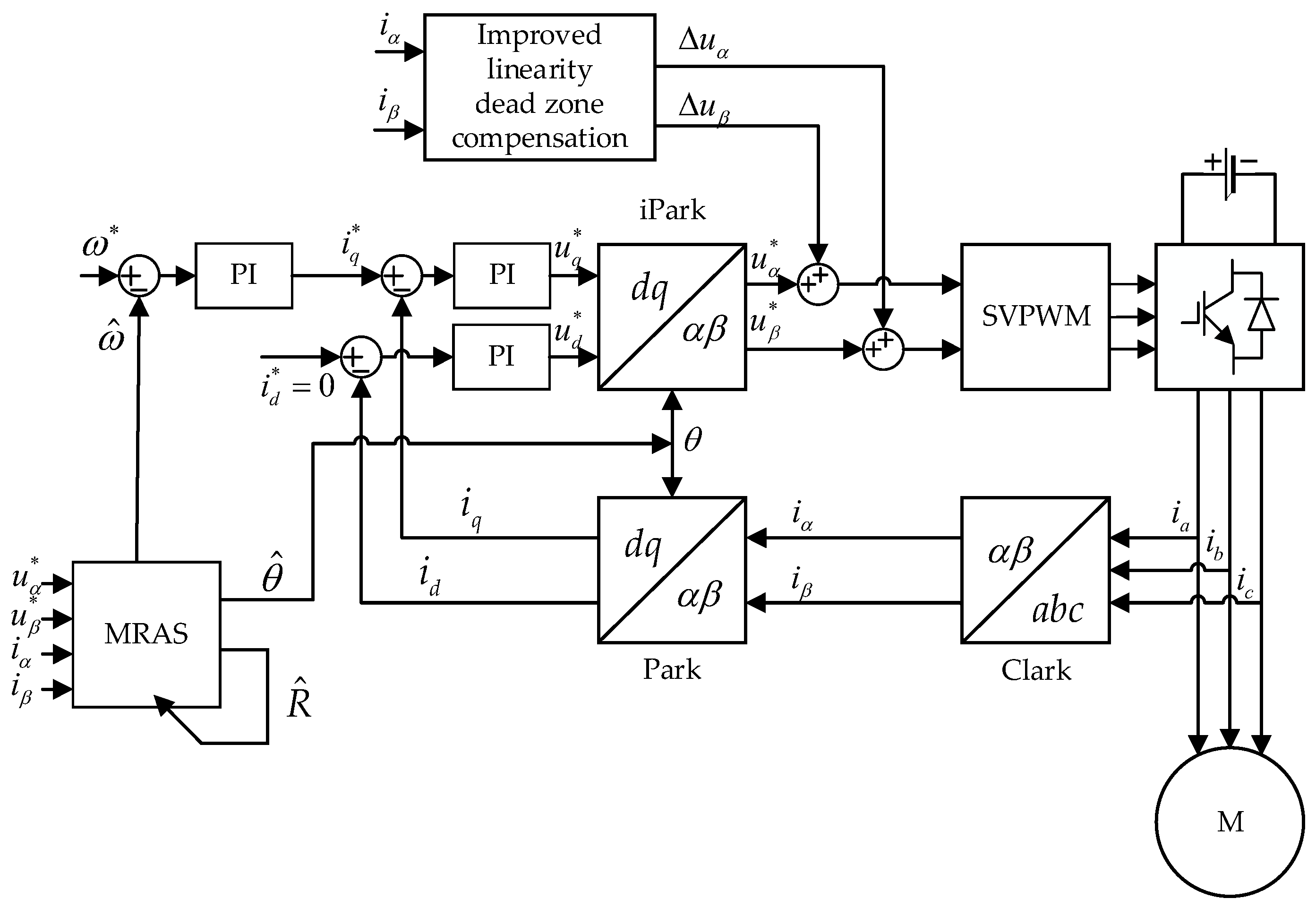
2. Resistance-Based Adaptive MRAS Speed Observation

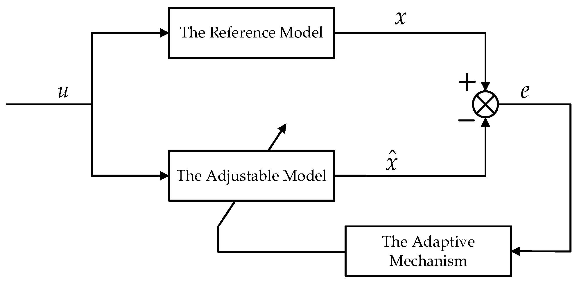
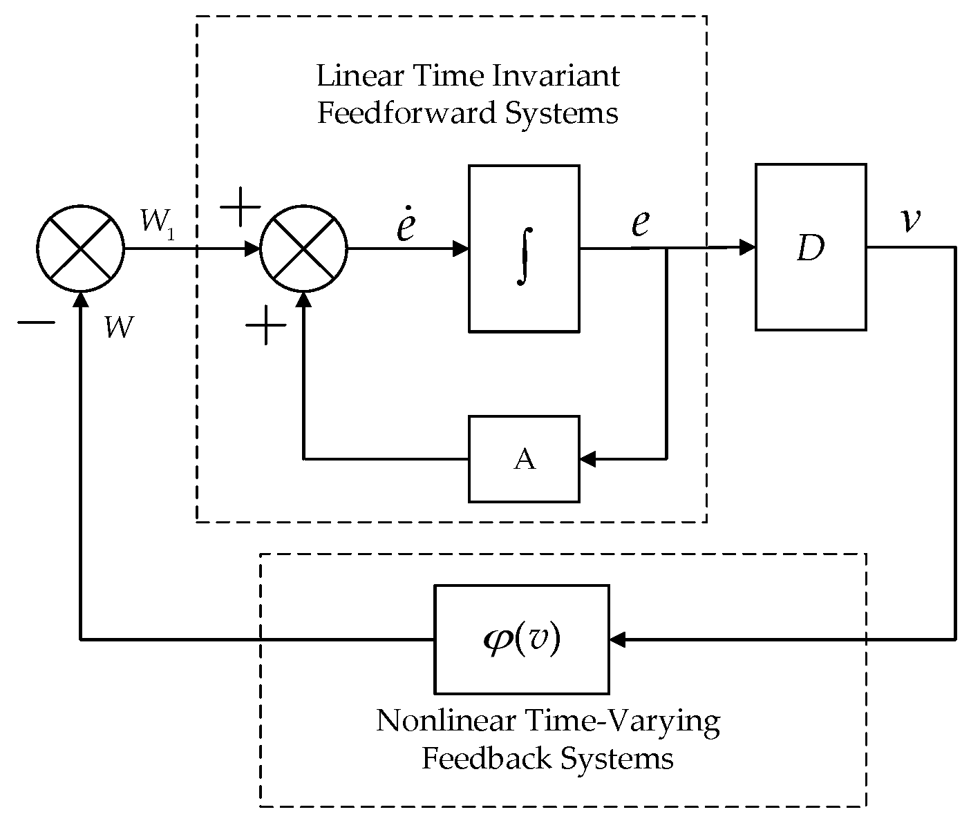
2.1. The Basic Principles of MRAS

An MRAS consists of three basic modules: a reference model, an adjustable model, and an adaptive mechanism. As shown in Figure 1, the reference model and the adjustable model are connected in parallel and are excited by the same external input $u$. The reference model and the adjustable model are connected in parallel. The output $\hat{x}$ of the adjustable model converges to the output of the reference model. The error in the outputs of the two models is adjusted by the adaptive law to generate an adjustment signal to update the parameters in the adjustable model, so that the output $\hat{x}$ of the adjustable model can quickly and stably approximate the output $x$ of the reference model, realizing the purpose of dynamic tracking.

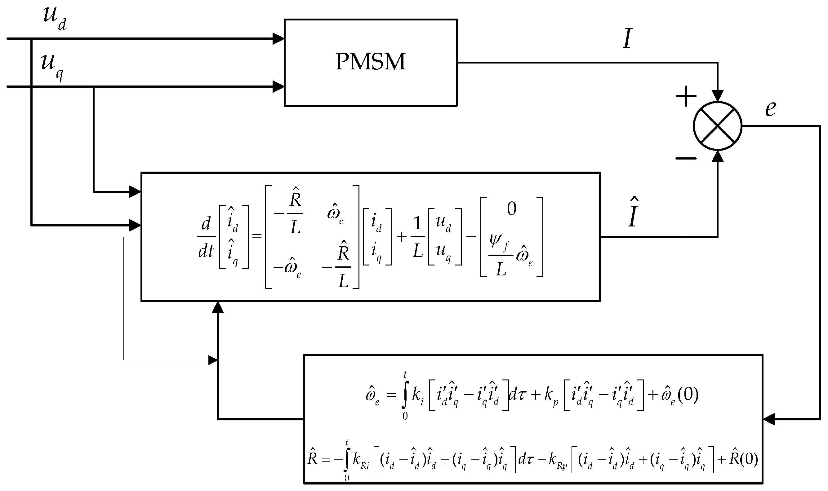
2.2. Resistance Identification and Speed Observation Model

A permanent magnet synchronous motor is a multivariable, strongly coupled, nonlinear, time-varying complex system. The following assumptions need to be made in its mathematical modeling: (1) the induced electromotive force in the motor phase windings is sinusoidal; (2) there is no damping winding on the motor rotor; and (3) core saturation can be ignored, and motor core losses can be ignored.

Under the above assumptions, the differential equation for the stator current of a tabular permanent magnet synchronous motor ($L_d=L_q=L$) in the d-q frame is:

$$\frac{d}{dt}\left[\begin{array}{c}{i}_d\\ i_q\end{array}\right]=\left[\begin{array}{cc}-\frac{R}{L}& {\omega }_e\\ -{\omega }_e& -\frac{R}{L}\end{array}\right]\left[\begin{array}{c}{i}_d\\ i_q\end{array}\right]+\frac{1}{L}\left[\begin{array}{c}{u}_d\\ u_q\end{array}\right]-\left[\begin{array}{c}0\\ \frac{{\psi }_f}{L}{\omega }_e\end{array}\right]$$

(1)

where $u_d$, $u_q$, $i_d$, and $i_q$ are the dq-axis stator voltage components and current components; $R$ is the stator resistance; $L$ is the stator inductance; ${\psi }_f$ is the rotor magnetic flux linkage; and ${\omega }_e$ is rotor electrical speed.

Equation (1) is equivalent to:

$$\frac{d}{dt}\left[\begin{array}{c}{i}_d+\frac{{\psi }_f}{L}\\ i_q\end{array}\right]=\left[\begin{array}{cc}-\frac{R}{L}& {\omega }_e\\ -{\omega }_e& -\frac{R}{L}\end{array}\right]\left[\begin{array}{c}{i}_d+\frac{{\psi }_f}{L}\\ i_q\end{array}\right]+\frac{1}{L}\left[\begin{array}{c}{u}_d+\frac{R{\psi }_f}{L}\\ u_q\end{array}\right]$$

(2)

Assuming that $i_d^{\prime }=i_d+\frac{{\psi }_f}{L}$, $i_q^{\prime }=i_q$, $u_d^{\prime }=u_d+\frac{R{\psi }_f}{L}$, $u_q^{\prime }=u_q$:

$$\frac{d}{dt}\left[\begin{array}{c}{i}_d^{\prime }\\ i_q^{\prime }\end{array}\right]=\left[\begin{array}{cc}-\frac{R}{L}& {\omega }_e\\ -{\omega }_e& -\frac{R}{L}\end{array}\right]\left[\begin{array}{c}{i}_d^{\prime }\\ i_q^{\prime }\end{array}\right]+\frac{1}{L}\left[\begin{array}{c}{u}_d^{\prime }\\ u_q^{\prime }\end{array}\right]$$

(3)

In order to identify the motor speed and resistance, the PMSM itself can be chosen as the reference model and the current equation as the adjustable model. Based on the analysis above, the mathematical model of the PMSM is first expressed in the form of a nonlinear feedback system combining a linear constant forward loop and a nonlinear constant feedback loop. Equation (3) can be rewritten as:

$$\frac{d}{dt}{i}^{\prime }=A{i}^{\prime }+B{u}^{\prime }$$

(4)

where $i^{\prime }$ is the actual motor current state vector, $i^{\prime }={\left[\begin{array}{cc}{i}_d^{\prime }& i_q^{\prime }\end{array}\right]}^T$ and $u^{\prime }$ is the actual motor voltage state vector, $u^{\prime }={\left[\begin{array}{cc}{u}_d^{\prime }& u_q^{\prime }\end{array}\right]}^T$.

Expressing Equation (3) in terms of estimates, we obtain an adjustable model for the parallel connection:

$$\frac{d}{dt}\left[\begin{array}{c}{\hat{i}}_d^{\prime }\\ {\hat{i}}_q^{\prime }\end{array}\right]=\left[\begin{array}{cc}-\frac{\hat{R}}{L}& {\hat{\omega }}_e\\ -{\hat{\omega }}_e& -\frac{\hat{R}}{L}\end{array}\right]\left[\begin{array}{c}{\hat{i}}_d^{\prime }\\ {\hat{i}}_q^{\prime }\end{array}\right]+\frac{1}{L}\left[\begin{array}{c}{\hat{u}}_d^{\prime }\\ {\hat{u}}_q^{\prime }\end{array}\right]$$

(5)

Equation (5) is simplified as:

$$\frac{d}{dt}{\hat{i}}^{\prime }=A{\hat{i}}^{\prime }+B{\hat{u}}^{\prime }$$

(6)

Assume $e=i^{\prime }-{\hat{i}}^{\prime }$; if we subtract Equation (5) from Equation (3), the error state equation can be obtained:

$$\frac{d}{dt}e=Ae-Iw$$

(7)

A Popov nonlinear feedback system is established according to Equation (7), as shown in Figure 2, and in order to ensure the positivity of the transfer function of the forward constant channel, a linear compensator, D, is introduced into the system. D is the gain matrix, which is taken here as $D=I$ (unit vector). Then, $v=De$ and the expression $\phi (v)$ satisfies the Popov integral inequality. In order to prevent the regulation effect from being lost as the state generalized error $e$ gradually tends to zero, the adaptive law of the parameters is designed in the form of PI. It is worth noting that Lyapunov’s V-function is not easy to find when analyzing the stability of a closed-loop system consisting of nonlinear feedback links, whereas Popov’s stability theory has a general approach, and is therefore particularly suitable for the design of MRASs.

It can be seen from the above that in the Popov integral inequality $v^T=e^T$, according to the Popov ultra-stable theory, if the system is asymptotically stable, the nonlinear time-varying link shown in Figure 2 must satisfy the Popov Equality (8):

$$\eta (0,t_1)={\displaystyle \underset{0}{\overset{t_1}{\int }}{V}^{T}Wdt\ge -{\gamma }^2},\forall t_1>0$$

(8)

where ${\gamma }^2$ is a finite positive number.

It can be seen from the above that $W=\Delta \hat{A}{i}^{\prime }+B({\hat{u}}^{\prime }-u^{\prime })$ and $B({\hat{u}}^{\prime }-u^{\prime })={\left[\begin{array}{cc}{\phi }_f(\hat{R}-R)/L^2& 0\end{array}\right]}^T$, and thus:

$$\Delta A=\hat{A}-A=\left[\begin{array}{cc}0& 1\\ -1& 0\end{array}\right]({\hat{\omega }}_e-{\omega }_e)-\left[\begin{array}{cc}1& 0\\ 0& 1\end{array}\right]\frac{\hat{R}-R}{L}$$

(9)

Assuming $J=\left[\begin{array}{cc}0& 1\\ -1& 0\end{array}\right]$, then substituting $V$ and $W$ into Equation (9) we obtain:

$$\eta (0,t_1)={\displaystyle \underset{0}{\overset{t_1}{\int }}{e}^T({\hat{\omega }}_e-{\omega }_e)}J{\hat{i}}^{\prime }dt+{\displaystyle \underset{o}{\overset{t_1}{\int }}-e^T}\frac{\hat{R}-R}{L}\left[\begin{array}{c}{i}_d\\ i_q\end{array}\right]\ge -{\gamma }^2$$

(10)

Equation (10) can be decomposed into two partial equations (Equations (11) and (12)).

$${\eta }_1(0,t_1)={\displaystyle \underset{0}{\overset{t_1}{\int }}{e}^T({\hat{\omega }}_e-{\omega }_e)}J{\hat{i}}^{\prime }dt\ge -{\gamma }^2$$

(11)

$${\eta }_2(0,t_1)={\displaystyle \underset{o}{\overset{t_1}{\int }}-e^T}\frac{\hat{R}-R}{L}\left[\begin{array}{c}{i}_d\\ i_q\end{array}\right]\ge -{\gamma }^2$$

(12)

The observed speed is solved by Equation (11), and the identified resistance is solved by Equation (12). Taking the observed speed ${\hat{\omega }}_e$ as an example, the adaptive law in the form of PI is:

$${\hat{\omega }}_e={\hat{\omega }}_e(0)+{\displaystyle \underset{0}{\overset{t}{\int }}{G}_1(\tau )d\tau +}{G}_2(\tau )$$

(13)

Bringing Equation (13) into Equation (11) yields:

$$\begin{array}{cc}\hfill {\eta }_1(0,t_1)=& {\displaystyle \underset{0}{\overset{t_1}{\int }}{e}^T\left[{\omega }_e-{\displaystyle \underset{0}{\overset{t}{\int }}{G}_1\left(\tau \right)d\tau -{\hat{\omega }}_e\left(0\right)}\right]}J{\hat{i}}^{\prime }dt+{\displaystyle \underset{0}{\overset{t_1}{\int }}{e}^T{G}_2\left(\tau \right)J{\hat{i}}^{\prime }dt}\hfill \\ \hfill =& {\eta }_1^{\prime }(0,t_1)+{\eta }_2^{\prime }(0,t_1)\hfill \\ \hfill \ge & -{\gamma }_1{}^2-{\gamma }_2{}^2\hfill \\ \hfill =& -{\gamma }_0{}^2\hfill \end{array}$$

(14)

When ${\eta }_1^{\prime }(0,t_1)\ge -{\gamma }_1{}^2$ and ${\eta }_2^{\prime }(0,t_1)\ge -{\gamma }_2{}^2$ are established separately, then Equation (14) is established.

Assume $\frac{d}{dt}f\left(t\right)=e^{T}J{\hat{i}}^{\prime }$ and $kf\left(t\right)={\omega }_e-{\displaystyle \underset{0}{\overset{t}{\int }}{G}_1\left(\tau \right)d\tau -}{\hat{\omega }}_e(0)$; then:

$${\displaystyle \underset{0}{\overset{t}{\int }}\frac{d}{dt}f\left(t\right)}kf\left(t\right)dt=\frac{k}{2}{f}^2\left(t\right)\ge 0$$

(15)

Therefore, when $G_1\left(\tau \right)=k_i{e}^{T}J{\hat{i}}^{\prime }$, inequality ${\eta }_1^{\prime }(0,t_1)\ge -{\gamma }_1{}^2$ is established; when $G_1\left(\tau \right)=k_p{e}^{T}J{\hat{i}}^{\prime }$, inequality ${\eta }_2^{\prime }(0,t_1)\ge -{\gamma }_2{}^2$ is established.

From the above analysis, the adaptive rate of ${\hat{\omega }}_e$ can be obtained:

$${\hat{\omega }}_e={\hat{\omega }}_e(0)+{\displaystyle \underset{0}{\overset{t}{\int }}{k}_i\left[i_d^{\prime }{\hat{i}}_q^{\prime }-i_q^{\prime }{\hat{i}}_d^{\prime }\right]}d\tau +k_p\left[i_d^{\prime }{\hat{i}}_q^{\prime }-i_q^{\prime }{\hat{i}}_d^{\prime }\right]$$

(16)

Similarly, the adaptive rate of $\hat{R}$ as follows:

$$\hat{R}=\hat{R}(0)-{\displaystyle \underset{0}{\overset{t}{\int }}{k}_{Ri}}\left[(i_d-{\hat{i}}_d){\hat{i}}_d+(i_q-{\hat{i}}_q){\hat{i}}_q\right]d\tau -k_{Rp}\left[(i_d-{\hat{i}}_d){\hat{i}}_d+(i_q-{\hat{i}}_q){\hat{i}}_q\right]$$

(17)

The structure of the reference model, adjustable model, and adaptive law of the PMSM model reference adaptive system is shown in Figure 3, where $I$ is the sampling current and $\hat{I}$ is the estimated current.

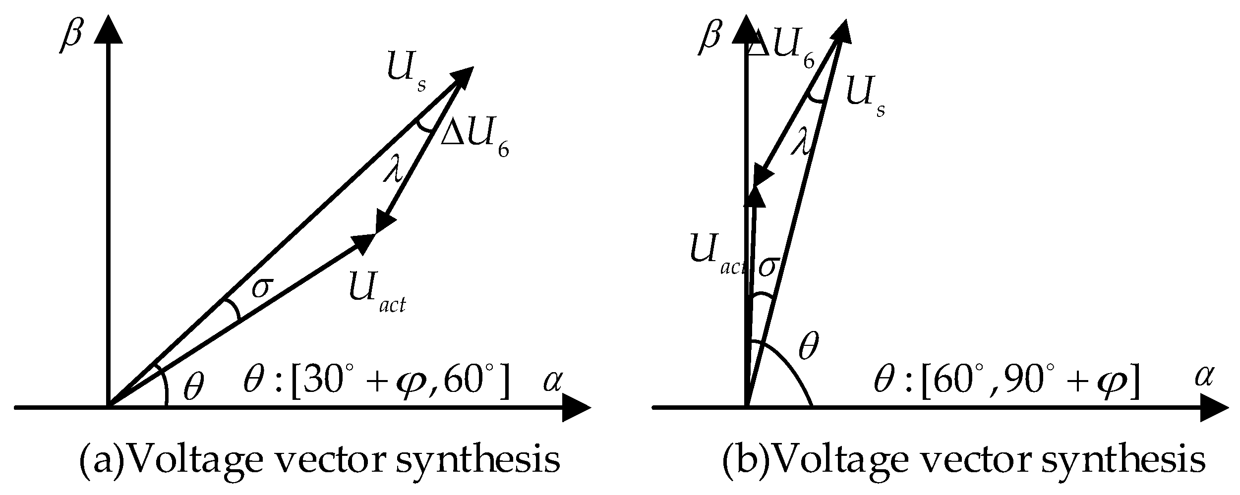
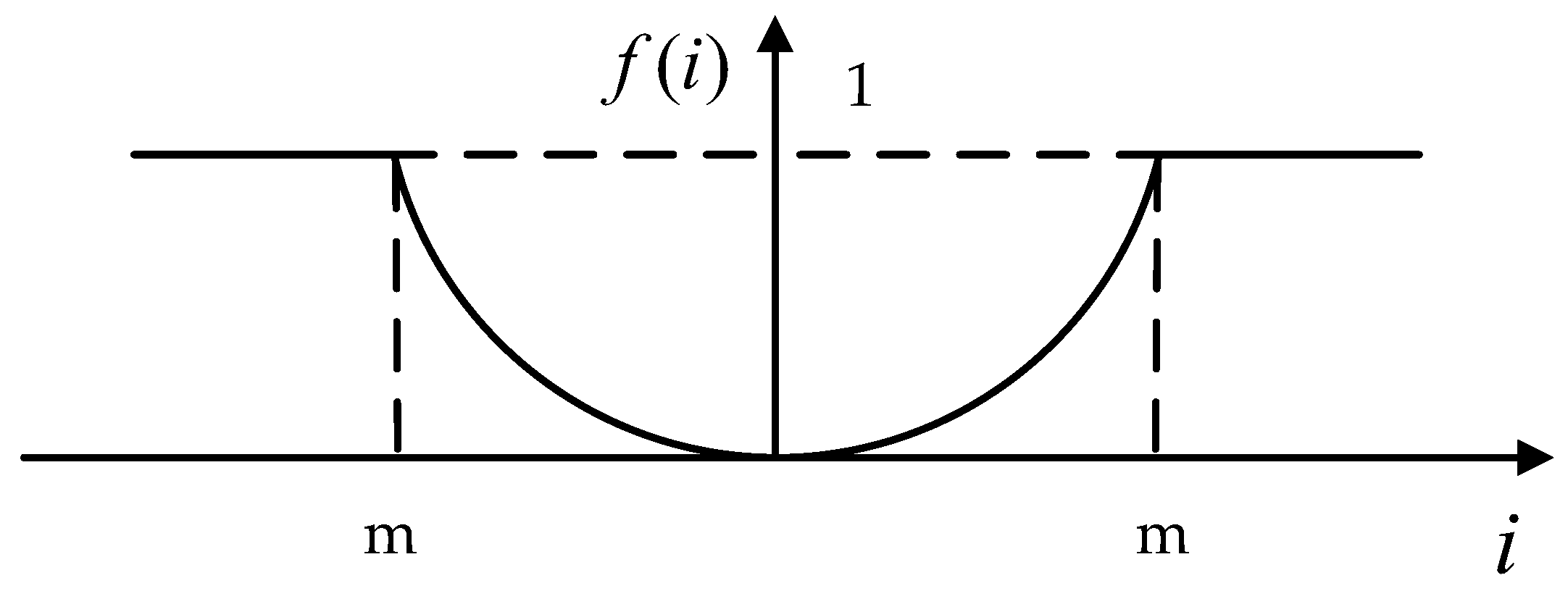
3. Dead Zone Effect on Observation Error

The non-ideal characteristics of the power tube switching lead to the nonlinearity of the actual output voltage of the inverter, which is reflected in the loss of the fundamental voltage of the output, the increase in harmonics, the distortion of the output current, and torque pulsation [16,17]. Considering the voltage error between the inverter output voltage and the actual voltage, the actual voltage vector $U_{act}$ can be expressed as:

$$U_{act}=U_s+\Delta U_i$$

(18)

where $U_s$ is the target voltage vector and $\Delta U_i$ is the error voltage vector, whose direction is shown in Figure 4 and magnitude is equal to the magnitude second to $\frac{T_d}{T_s}{U}_s$. The direction of the error voltage vector is determined by the polarity of the sampling current, with the direction of current flow toward the load denoted as positive. When the polarity of $i_a,i_b,i_c$ are positive, positive, and negative, the error voltage vector corresponds to $\Delta U_6$.

The stator current vector in the above case is at $\left[{30}^{\circ },{90}^{\circ }\right]$, assuming that the angle of voltage vector $U_s$ is $\phi$ and the phase $\theta$ of $U_s$ is at $\left[{30}^{\circ }+\phi ,{90}^{\circ }+\phi \right]$. The actual voltage vector $U_{act}$ is synthesized as in Figure 5; note that the angle between $U_s$ and $U_{act}$ is $\sigma$, and the angle between the error voltage $\Delta U_6$ and $U_s$ is $\lambda$.

When $\theta$ is at $\left[{30}^{\circ }+\phi ,{60}^{\circ }\right]$ in Figure 5a, the angle $\lambda$ as follows:

$$\lambda ={60}^{\circ }-\theta$$

(19)

Then, the amplitude of $U_{act}$ is:

$$\left|U_{act}\right|=\sqrt{{\left|U_s\right|}^2+{\left|\Delta U_6\right|}^2-2\left|U_s\right|\left|\Delta U_6\right|\cos \lambda }$$

(20)

Meanwhile, the phase of the actual voltage vector $U_{act}$ that lags behind the given voltage vector $U_s$ is $\sigma$:

$$\sigma =\arcsin (\left|\Delta U_6\right|·\sin \lambda /\left|U_{act}\right|)$$

(21)

The phase of the actual voltage vector $U_{act}$ can be obtained as:

$${\theta }_{act}=\theta -\sigma$$

(22)

Similarly, in Figure 5b, when $\theta$ is at $\left[{60}^{\circ },{90}^{\circ }+\phi \right]$, the angle $\lambda$ is $\lambda =\theta -{60}^{\circ }$ and ${\theta }_{act}$ can be obtained from ${\theta }_{act}=\theta +\sigma$.

Similarly, the actual voltage vectors under the other five sets of current polarizations can be obtained. Assuming that the amplitude of $T_d$ = 7 us, $U_{dc}$ = 310 V, $T_s$ = 100 us, and error voltage $\Delta U_i$ is 21.7 V, the amplitude of $U_s$ is 100 V, and leads the stator current vector to be 15°. The simulation yields are shown Figure 6. There is a large difference between the waveforms of $U_s$ and $U_{act}$ in the two-phase stationary coordinate system in (a) and in the time domain in (d), which is affected by the dead zone with a steep change in the angle (see Figure 6c) and amplitude of $U_{act}$ with respect to $U_s$.

It can be seen that there is a large difference between the given voltage $U_s$ and the actual voltage $U_{act}$, and the MRAS uses the voltage given by the inner loop of the current to perform the speed observation and resistance identification, so it is necessary to introduce the dead zone compensation to reduce the deviation between the actual voltage and the given voltage to improve the accuracy of the MRAS observations.

Dead zone compensation in the current polarity judgment is difficult since motor operation in the three-phase current contains more harmonics and cannot be directly measured through the sampling value of the current polarity judgment. Therefore, in this study, the DC component of the current under the synchronous rotation system was processed according to the phase judgment of the current polarity, combined with the current polarity in the two-phase stationary coordinate system to give the compensation signal (Figure 7).

$${\left[\begin{array}{cc}{U}_{\alpha }& U_{\beta }\end{array}\right]}^T=f(i)\cdot {\left[\begin{array}{cc}\Delta U_{\alpha }& \Delta U_{\beta }\end{array}\right]}^T$$

(23)

In practice, the current in the zero point is not useful in determining the polarity; a judgment error will aggravate the dead zone effect so that the current distortion is more serious. Therefore, to perform dead zone compensation using improved linear compensation scheme in the current over the zero point, the compensation gain in the form of a quadratic function near the zero point, as shown in Figure 8. $m$ is the modulation ratio, and this paper set the rated current to 4%; thus, the program can effectively avoid the risk of deterioration of the compensation due to the error in judging the current polarity.

$$f(i)=\{\begin{array}{ll}sign(i)\cdot {\left(\frac{i}{m}\right)}^2& \left|i\right|<m\\ sign(i)& \left|i\right|\ge m\end{array}$$

(24)

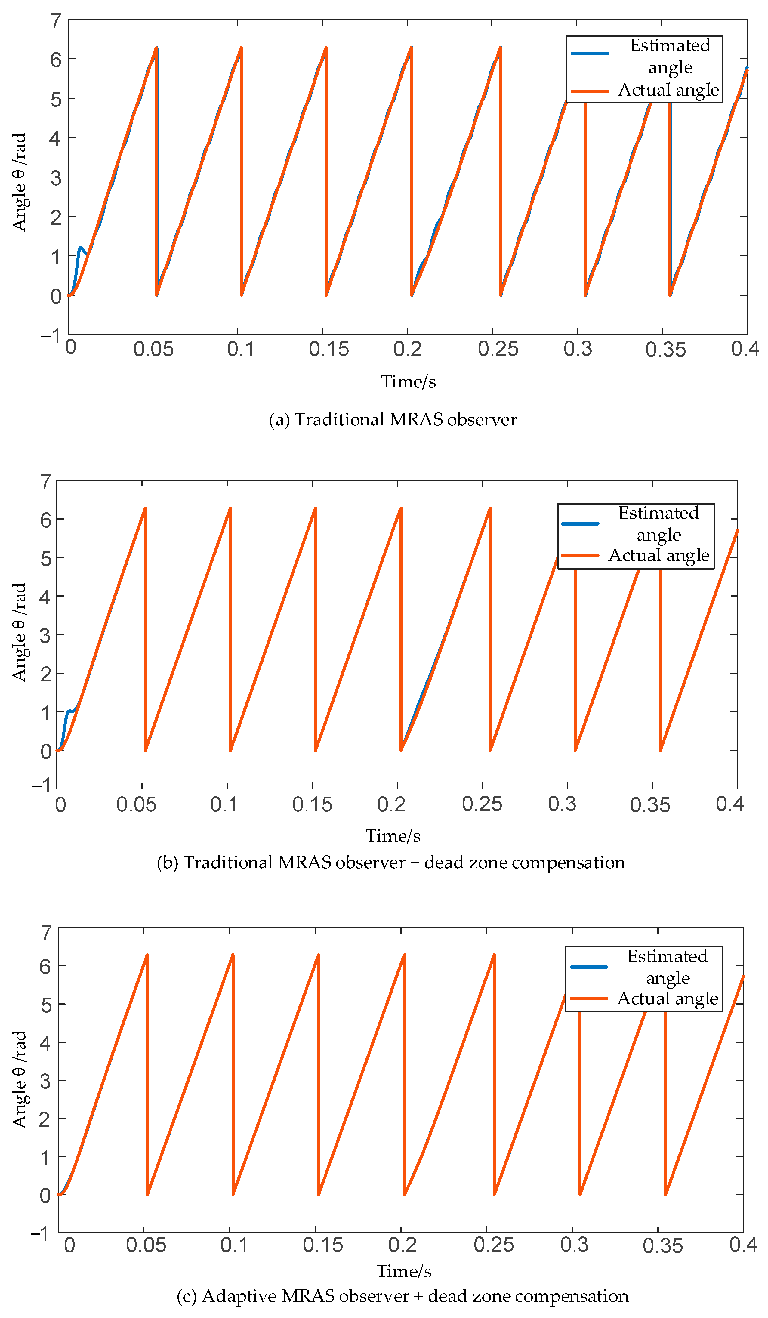
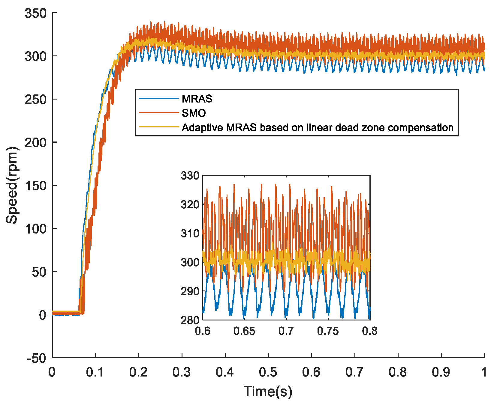
4. Simulation Result Analysis

The principle block diagram of the adaptive MRAS observer based on improved linear dead zone compensation is shown in Figure 9. The speed observer based on the MRAS is constructed to feed back the speed and angle information of the observer to realize the closed loop of the system. Meanwhile, the MRAS is used to conduct the online recognition of the resistance, and the voltage equations can satisfy the requirements of the speed observation and the recognition of the resistance rank at the same time, and the recognized resistance is fed back to the observer to improve the observation accuracy. When the motor is running at a low speed, the three-phase currents are collected through low-end sampling, converted to two-phase static coordinate system currents as inputs to the dead zone compensation module, and combined with the proposed compensation scheme; the two-phase static coordinate system voltage output from the current PI loop are compensated, so as to improve the accuracy of the observer when the motor is running at a low speed.

The simulation was verified in Matlab/Simulink and the motor parameters are shown in

Table 1. Motor parameters.

Parameter	Value
Rated line voltage (V)	310
Rated line current (A)	3
Rated power (W)	750
Rated speed (r/min)	2500
Stator phase resistance (Ω)	1.68
Inductance (mH)	3.2
Permanent magnet flux linkage (Wb)	0.093
Number of pole pairs	4

.

A surface-mounted permanent magnet synchronous motor was used, with $i_d=0$ control, a simulation time of 0.4 s, a simulation step size of 0.001 s, a rotational speed of 300 r/min, and a load torque of 2.5 $\mathrm{N}·\mathrm{m}$ was applied abruptly at 0.2 s.

Figure 10 shows the simulated waveforms of the resistance discrimination of the adaptive MRAS observer before and after the improved linear dead zone compensation, under a dead zone time of 7 μs, which changes the motor resistance from 1.68 Ω to 3 Ω at 0.2 s. Figure 10a shows that, when dead zone compensation is not performed, the discrimination of the resistance had a large error and fluctuated significantly in the steady state, and Figure 10b shows that, after the introduction of the dead zone compensation, the resistance discrimination had an error within the range of 0.05 Ω, indicating that the proposed improved linear dead zone compensation scheme improved the effect of online resistance identification.

Figure 11, Figure 12 and Figure 13 show the rotational speed, angle, and dq-axis current waveforms of the conventional MRAS observer and the improved adaptive MRAS observer for an initial value of 3 Ω of the resistor and a dead time of 7 μs. In Figure 11a, the rotational speed observation of the conventional MRAS had a deviation of 50 r/min, which is a poor performance. In Figure 11b, the conventional MRAS observer had a significant improvement with a rotational speed error within 10 r/min using the improved linear dead time compensation. In Figure 11c, based on the online identification of the resistor and the real-time correction of the parameters of the observer, the speed error was controlled within 2 r/min, and the observation effect was further improved. In Figure 12, the traditional MRAS observer had a large deviation in the electrical angle estimation during the startup and sudden load change, and after improving the linear dead zone compensation and resistance identification, the observation angle effect was also greatly improved. In Figure 13a, the dq-axis current and motor torque fluctuated greatly under the traditional MRAS control, and the overall control effect of the motor was poor. With the addition of the improved linear dead zone compensation in Figure 13b, the dq-axis current and torque fluctuations were significantly improved, and in Figure 13c, the current and torque control was further improved after the introduction of online resistor identification.

The dead zone effect and the variation in the actual resistance value of the motor at low speeds with load will affect the observation accuracy of angle and speed, and the control of current is not ideal, which affects the efficiency of the motor. The proposed adaptive MRAS observer with improved linear dead zone compensation can ensure that these problems can be solved under the stable convergence of the algorithm. The improved dead zone compensation scheme not only improves the control effect of the motor at low speeds, but also improves the accuracy of the online identification of the resistance, and the combination of the two schemes also improves the efficiency of the motor at low speeds and under a load.

5. Experimental Verification

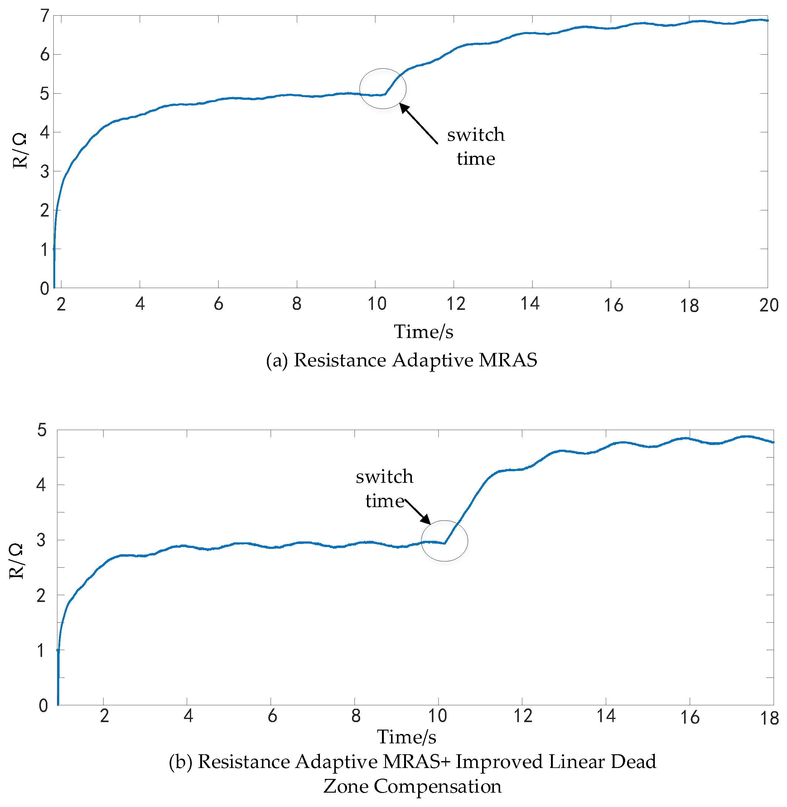
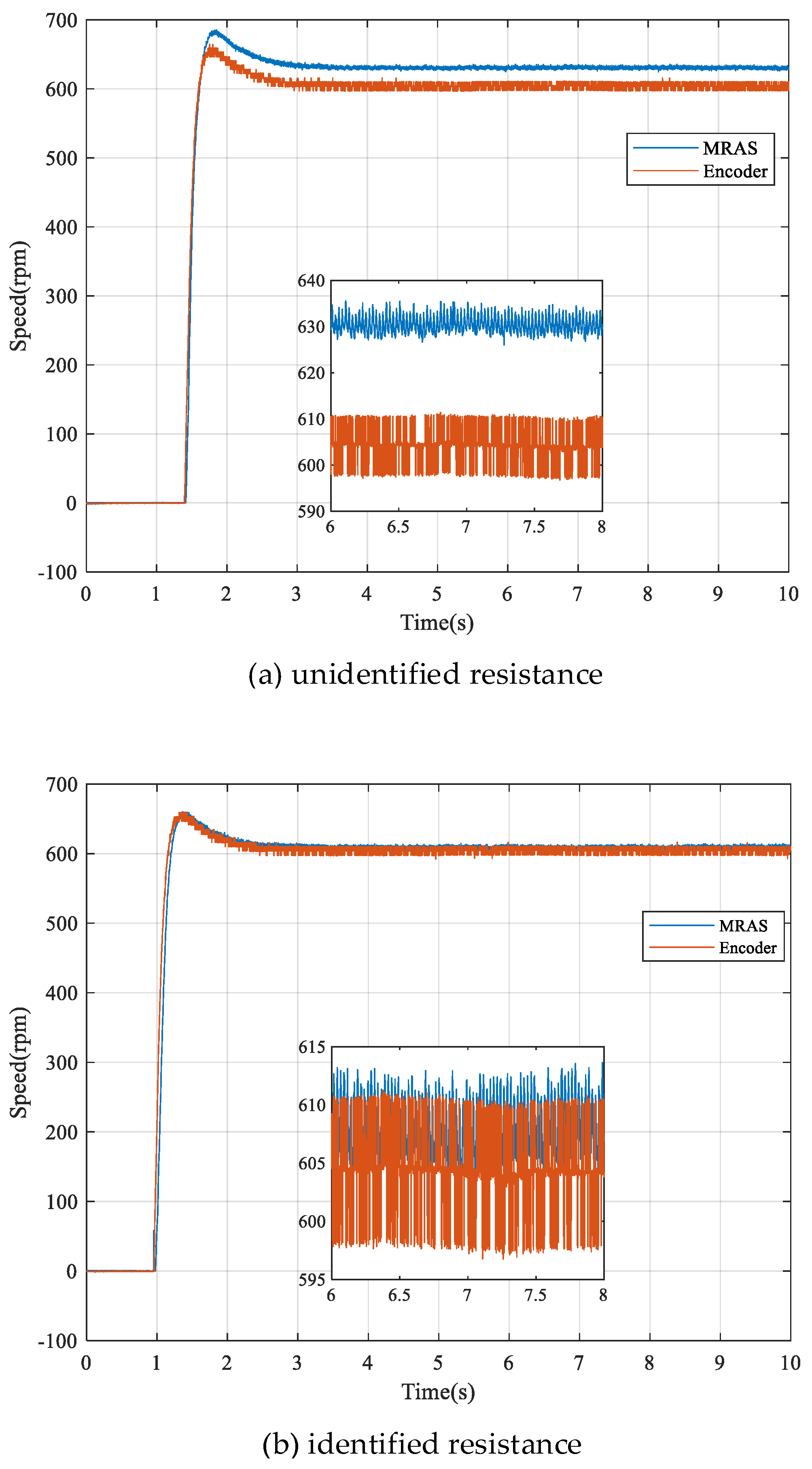
5.1. MRAS Resistance Identification

The field orientation control (FOC) strategy based on “Id = 0” was employed, and the control strategy was implemented using a TMS320F28335 digital signal processor. The PWM switching frequency and the current sampling frequency were set to 10 kHz. The parameters of the test PMSM are listed in Table 1.

The vector control experimental platform based on DSP28335 was constructed, as shown in Figure 14 below.

First, the MRAS-based resistance identification designed in this paper was experimentally verified. The switching resistor was set to 2 Ω, with one end connected to the phase line of the test motor, and the other end connected to the three-phase output of the power board, which are connected in parallel with a wire; the switch is connected in series to the wire, and when the switch is closed, the switching resistor is shorted, and when the switch is open, the switching resistor is connected in series to the three-phase output.

In the absence of dead zone compensation in the case of MRAS resistance identification effect (Figure 15a), due to the inverter dead zone effect, the low-speed resistance identification is poor, and is greater than the actual resistance of 2–4 Ω. Figure 15b shows that, after the improvement of the linear dead zone compensation, after the motor starts at 3 s, the resistance was identified accurately, the error was controlled in a range of 1 Ω or less, and the motor phase resistance in the 10.5 s change was more accurately and immediately identified. The resistance was also recognized accurately after changing the phase resistance of the motor at 10.5 s. This experiment shows that the dead zone compensation can effectively improve the resistance recognition effect at low speeds.

5.2. Resistance Adaptive MRAS Speed Observation

Figure 16 shows the experimental comparison between the MRAS speed observations and encoder speed measurements at a set speed of 600 r/min. It can be seen that the accuracy of the speed control of the MRAS in Figure 16a is poor without resistor identification. The accuracy of the speed control in Figure 16b is significantly improved after using the scheme proposed in this paper.

Figure 17 shows the start-up waveforms of the sliding mode observer (SMO), traditional MRAS, and adaptive MRAS based on linear dead zone compensation at 300 r/min under a light load. The sliding mode observer uses a switching function, which led to large fluctuations in speed, and the accuracy of the speed observation was not high because of the dead zone effect at low speeds and the resistance change under a load; the speed waveform of the traditional MRAS observer had relatively less fluctuation, which was better than that of the SMO, but there no improvement in the accuracy of the speed observation over that of the SMO. The two largest observation errors were roughly 8.3% and 6%, while the adaptive MRAS based on linear dead zone compensation had the smallest fluctuation in the observed speed. The adaptive MRAS based on linear dead zone compensation produced the smallest fluctuation in rotational speed and the smallest error, which was about 1.6%. The scheme proposed in this paper can greatly improve the operation of the rotational speed observer and increase the efficiency of the motor.

Figure 18 shows the experimental plot of the observer’s rotational speed at 300 r/min. The conventional MRAS in Figure 18a is the least effective without dead zone compensation, and the speed fluctuation was large in both a steady state and with loading. Figure 18b shows the results with resistance online identification, and it can be seen that the speed control effect improved and the speed fluctuation was reduced. Finally, 18c introduces the improved linear dead zone compensation with the resistance adaptive MRAS, and the speed control effect was further improved.

Figure 19 shows the experimental graph of the dq-axis current at 300 r/min. In Figure 19a, the traditional MRAS had the worst effect without dead zone compensation, and its dq-axis current fluctuation was the largest. Figure 19b shows that, by performing online resistance identification and modifying the resistance parameters of the MRAS in real time, the dq-axis current fluctuation decreased, the torque pulsation decreased, and the control effect was improved. Figure 19c shows that by introducing an improved linear dead zone compensation to the adaptive MRAS, the control effect of the dq-axis was further improved.

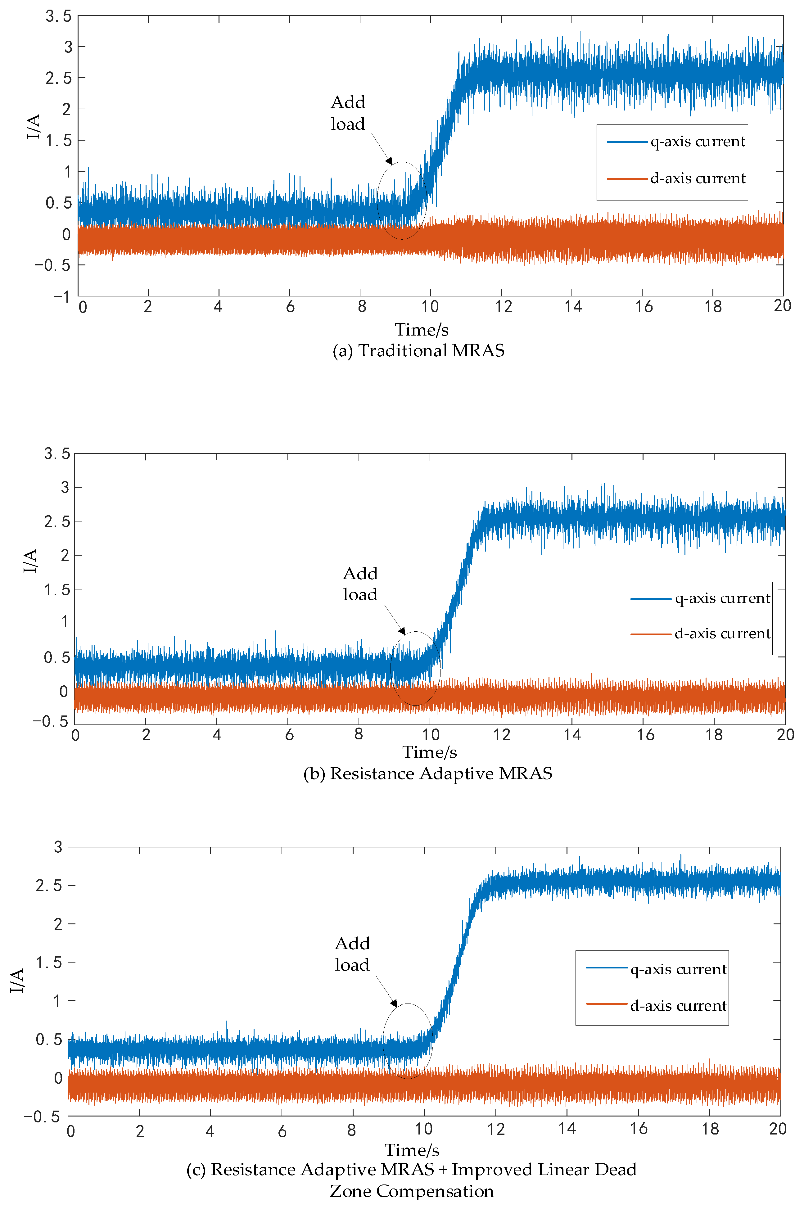
5.3. Experimental Verification of Improved Linear Dead Zone Compensation Effect

The phase currents before and after dead zone compensation and the corresponding spectra are shown in Figure 20 and Figure 21. Figure 20a shows the distortion of the phase current waveform without dead zone compensation at a low speed with a load, and the fifth and seventh harmonics can be seen in Figure 21a. Figure 20b shows that the conventional dead zone compensation improved the current sinusoidality but the compensation at the point of crossing zero was not significantly improved. From Figure 21b, it can be seen that the fifth and seventh harmonics were reduced, with some effect. As shown in Figure 20c, using the improved linear dead zone compensation method proposed in this paper, the sinusoidal degree of phase current was significantly improved, and the zero-clamping phenomenon was improved, and the proportions of the fifth and seventh harmonics were reduced (Figure 21c).

The improved linear dead zone compensation method proposed in this paper can significantly improve the motor operating conditions at low speeds with a load, effectively reducing the proportion of harmonic currents, increasing the fundamental wave component, and improving the over-zero clamping phenomenon.

6. Conclusions

In this paper, an adaptive MRAS observer based on improved linear dead zone compensation was proposed. The method utilizes MRAS to recognize the resistance online and observe the rotational speed. It uses an improved linear dead zone compensation to address the poor effect of the observer at low speeds with a load. This improvement enhances the observation accuracy of the MRAS by compensating for the dead zone voltage and, at the same time, improves the recognition accuracy of the resistance. The simulation and experimental results proved the effectiveness of the proposed scheme. The speed error was controlled within 2 r/min at 300 r/min, and the dq-axis current and torque fluctuation were significantly improved compared with the ordinary MRAS. The efficiency of the low-speed loaded operation of the motor was improved, and the improved linear dead zone compensation method effectively reduced the proportion of harmonic currents and solved the problem of over-zero clamping. However, the observer will still be affected by changes in parameters such as inductance and magnetic chain. The existing solution is to increase the rank of the system equations by injecting high-frequency signals to realize the multi-parameter identification. However, this approach is unfavorable to the dead zone compensation. Therefore, the compensation scheme of the dead zone under the injected signals is a topic that needs to be further researched.

References

1. Fadli, M.R.; Musyasy, M.M.; Furqani, J.; Purwadi, A. Modelling of Field Orientation Control (FOC) Method in 120 kW Brushless DC Motor (BLDC). In Proceedings of the 2019 6th International Conference on Electric Vehicular Technology (ICEVT), Bali, Indonesia, 18–21 November 2019; pp. 383–389. [Google Scholar]
2. Kojabadi, H.M.; Ghribi, M. MRAS-based adaptive speed estimator in PMSM drives. In Proceedings of the 9th IEEE International Workshop on Advanced Motion Control, Istanbul, Turkey, 27–29 March 2006; pp. 569–572. [Google Scholar]
3. Liu, Y.; Wan, J.; Li, G.; Yuan, C.; Shen, H. MRAS speed identification for PMSM based on fuzzy PI control. In Proceedings of the 2009 4th IEEE Conference on Industrial Electronics and Applications, Xi’an, China, 25–27 May 2009; pp. 1995–1998. [Google Scholar]
4. Dong, H.-Y.; Li, W.-G.; Zhao, Y.; Lin, K. Design and simulation a fuzzy-adaptive PI controller based on MRAS. In Proceedings of the 2010 Sixth International Conference on Natural Computation, Yantai, China, 10–12 August 2010; pp. 2321–2324. [Google Scholar]
5. Youlin, Y. A Speed Estimation Method with Stator Resistance Online Identification based on MRAS. In Proceedings of the 2019 Chinese Control and Decision Conference (CCDC), Nanchang, China, 3–5 June 2019; pp. 3697–3700. [Google Scholar]
6. Sreejeth, M.; Mehra, A. Estimation of stator resistance in sensor-less induction motor drive using MRAS. In Proceedings of the 2016 IEEE 1st International Conference on Power Electronics, Intelligent Control and Energy Systems (ICPEICES), Delhi, India, 4–6 July 2016; pp. 1–6. [Google Scholar]
7. Marković, I.; Erceg, I.; Sumina, D. MRAS based estimation of stator resistance and rotor flux linkage of permanent magnet generator considering core losses. In Proceedings of the IECON 2016—42nd Annual Conference of the IEEE Industrial Electronics Society, Florence, Italy, 24–27 October 2016; pp. 1948–1954. [Google Scholar]
8. Mehazzem, F.; Reama, A.; Benalla, H. Online rotor resistance estimation based on MRAS-sliding mode observer for induction motors. In Proceedings of the 4th International Conference on Power Engineering, Energy and Electrical Drives, Istanbul, Turkey, 13–17 May 2013; pp. 828–833. [Google Scholar]
9. Lipcak, O.; Bauer, J.; Chomat, M. Reactive Power MRAS for Rotor Resistance Estimation Taking into Account Load-Dependent Saturation of Induction Motor. In Proceedings of the 2019 International Conference on Electrical Drives & Power Electronics (EDPE), The High Tatras, Slovakia, 24–26 September 2019; pp. 255–260. [Google Scholar]
10. Khlaief, A.; Saadaoui, O.; Boussak, M.; Chaari, A. Implementation of stator resistance adaptation for sensorless speed control of IPMSM drive based on nonlinear position observer. In Proceedings of the 2016 XXII International Conference on Electrical Machines (ICEM), Lausanne, Switzerland, 4–7 September 2016; pp. 1071–1077. [Google Scholar]
11. Shi, Y.; Sun, K.; Ma, H.; Huang, L. Permanent magnet flux identification of IPMSM based on EKF with speed sensorless control. In Proceedings of the IECON 2010—36th Annual Conference on IEEE Industrial Electronics Society, Glendale, AZ, USA, 7–10 November 2010; pp. 2252–2257. [Google Scholar]
12. Ouyang, Y.; Dou, Y. Speed Sensorless Control of PMSM Based on MRAS Parameter Identification. In Proceedings of the 2018 21st International Conference on Electrical Machines and Systems (ICEMS), Jeju, Republic of Korea, 7–10 October 2018; pp. 1618–1622. [Google Scholar]
13. Ye, Z.; Liu, T.; Fuller, M.; Griepentrog, G. Parameter Identification of PMSM based on MRAS with Considering Nonlinearity of Inverter. In Proceedings of the IECON 2019—45th Annual Conference of the IEEE Industrial Electronics Society, Lisbon, Portugal, 14–17 October 2019; pp. 1255–1260. [Google Scholar]
14. Lin, H.; Marquez, A.; Wu, F.; Liu, J.; Luo, H.; Franquelo, L.G.; Wu, L. MRAS-Based Sensorless Control of PMSM with BPN in Prediction Mode. In Proceedings of the 2019 IEEE 28th International Symposium on Industrial Electronics (ISIE), Vancouver, BC, Canada, 12–14 June 2019; pp. 1755–1760. [Google Scholar]
15. Dong, D.; Xu, W.; Xiao, X.; Liu, Y. Online Magnetizing Inductance Identification Strategy of Linear Induction Motor Based on Second-Order Sliding-Mode Observer and MRAS. In Proceedings of the 2021 13th International Symposium on Linear Drives for Industry Applications (LDIA), Wuhan, China, 1–3 July 2021; pp. 1–6. [Google Scholar]
16. Ben-Brahim, L. On the compensation of dead time and zero-current crossing for a PWM-inverter-controlled AC servo drive. IEEE Trans. Ind. Electron. 2004, 51, 1113–1118. [Google Scholar] [CrossRef]
17. Sun, X.; Zhong, Y.; Ren, B.; Zhou, B. A Novel Measurement Method of Dead Zone Compensation Time. Proc. Chin. Soc. Electr. Eng. 2003, 23, 5. [Google Scholar]
Figure 1. MRAS model.
Electronics 12 04907 g001
Figure 2. Popov nonlinear feedback system.
Electronics 12 04907 g002
Figure 3. Model reference adaptive identification system of PMSM.
Electronics 12 04907 g003
Figure 4. Error voltage vector.
Electronics 12 04907 g004
Figure 5. Voltage vector synthesis when error voltage vector is Δ U 6 .
Electronics 12 04907 g005
Figure 6. Waveform of dead zone effect.
Electronics 12 04907 g006
Figure 7. Dead zone compensation scheme.
Electronics 12 04907 g007
Figure 8. Improved linear compensation function.
Electronics 12 04907 g008
Figure 9. Adaptive MRAS observer based on improved linear dead zone compensation.
Electronics 12 04907 g009
Figure 10. Resistance identification waveforms.
Electronics 12 04907 g010
Figure 11. Speed observation waveform.
Electronics 12 04907 g011
Figure 12. Angle observation waveform.
Electronics 12 04907 g012
Figure 13. dq-axis current waveform.
Electronics 12 04907 g013
Figure 14. Experiment platform.
Electronics 12 04907 g014
Figure 15. Resistance online identification.
Electronics 12 04907 g015
Figure 16. MRAS speed observation and encoder speed measurement.
Electronics 12 04907 g016
Figure 17. Speed start-up waveform at a low speed with a light load.
Electronics 12 04907 g017
Figure 18. Diagram of 300 r/min experiment.
Electronics 12 04907 g018
Figure 19. dq-axis current at 300 r/min.
Electronics 12 04907 g019
Figure 20. Phase current comparison before and after dead zone compensation.
Electronics 12 04907 g020
Figure 21. Spectrum comparison before and after dead zone compensation.
Electronics 12 04907 g021