
Deep Learning for Channel Estimation in Physical Layer Wireless Communications: Fundamental, Methods, and Challenges


Abstract
:1. Introduction
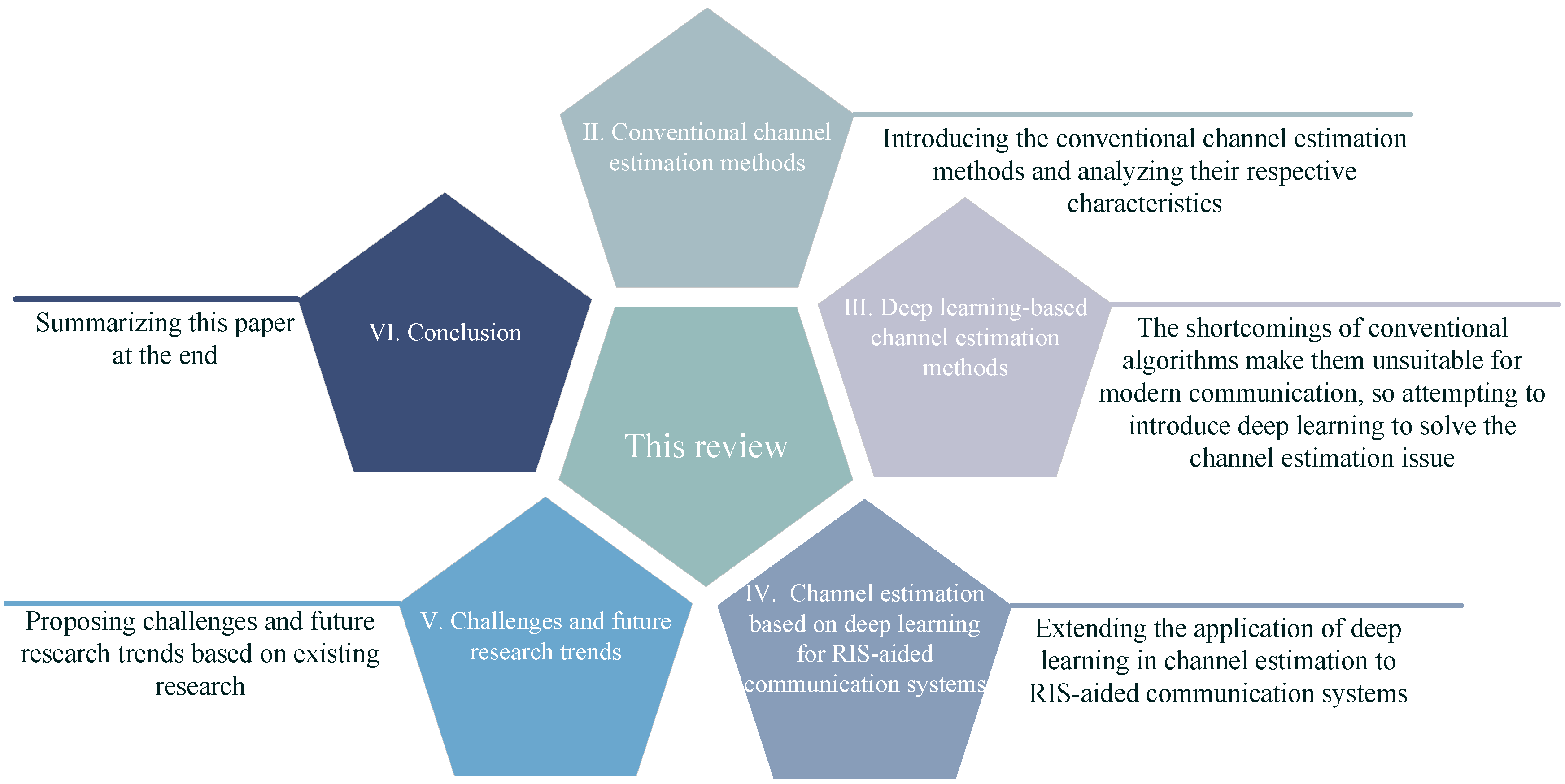
- Before discussing deep-learning-based channel estimation methods, conventional methods are introduced and classified as pilot-based, blind, and semi-blind, followed by an analysis of the advantages and disadvantages of each category.
- Dividing deep-learning-based channel estimation methods into data-driven and model-driven approaches, then reviewing their recent studies based on neural network types and benchmark algorithm types, respectively.
- We extend the discussion on applying deep learning to channel estimation to RIS-aided communication systems, which are emerging scenarios in next-generation wireless communications.
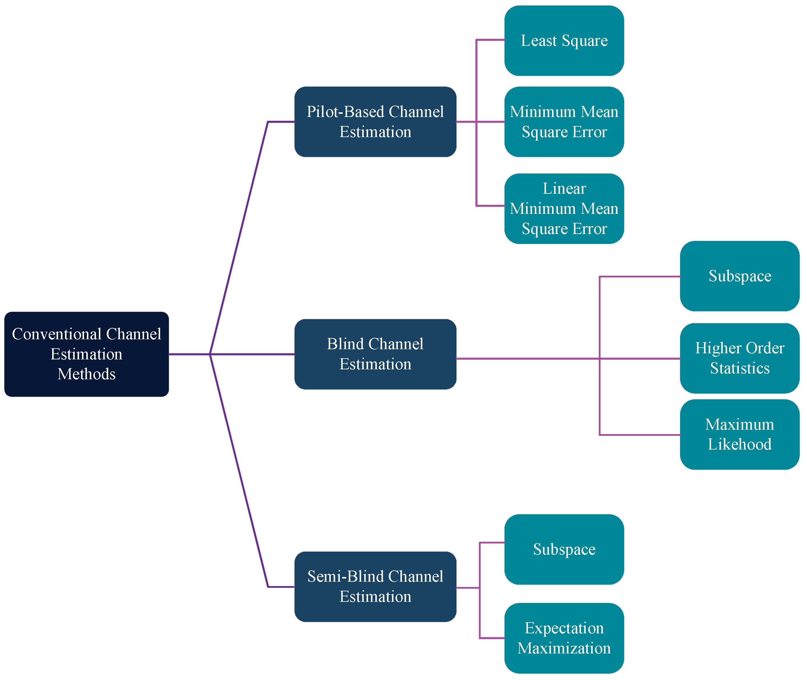
2. Conventional Channel Estimation Methods
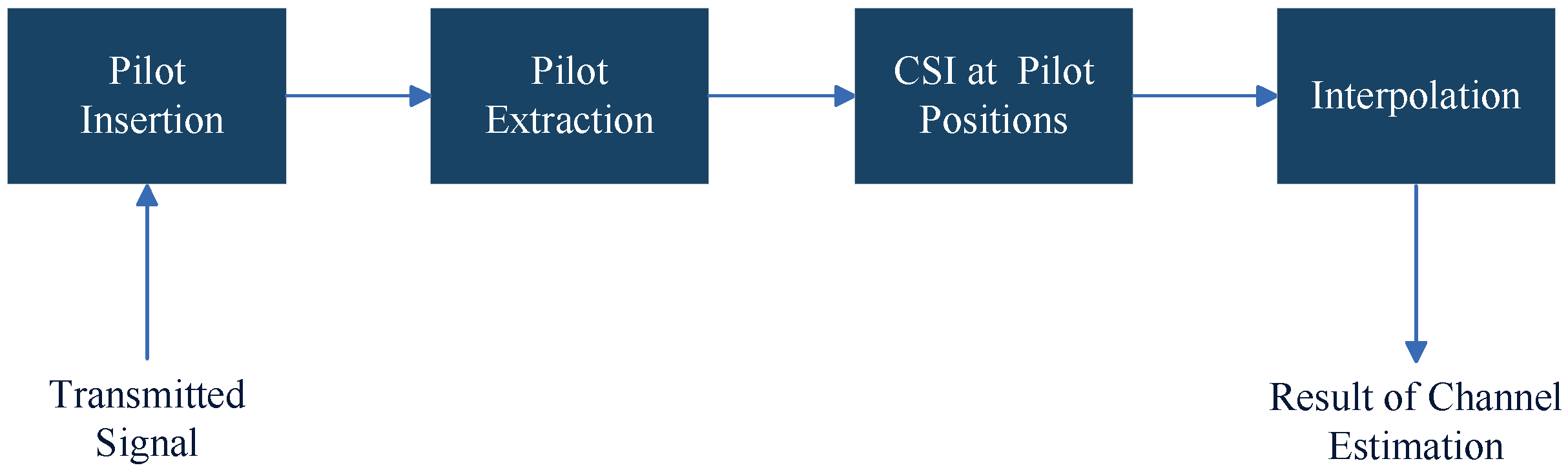
2.1. Pilot-Based Channel Estimation Method
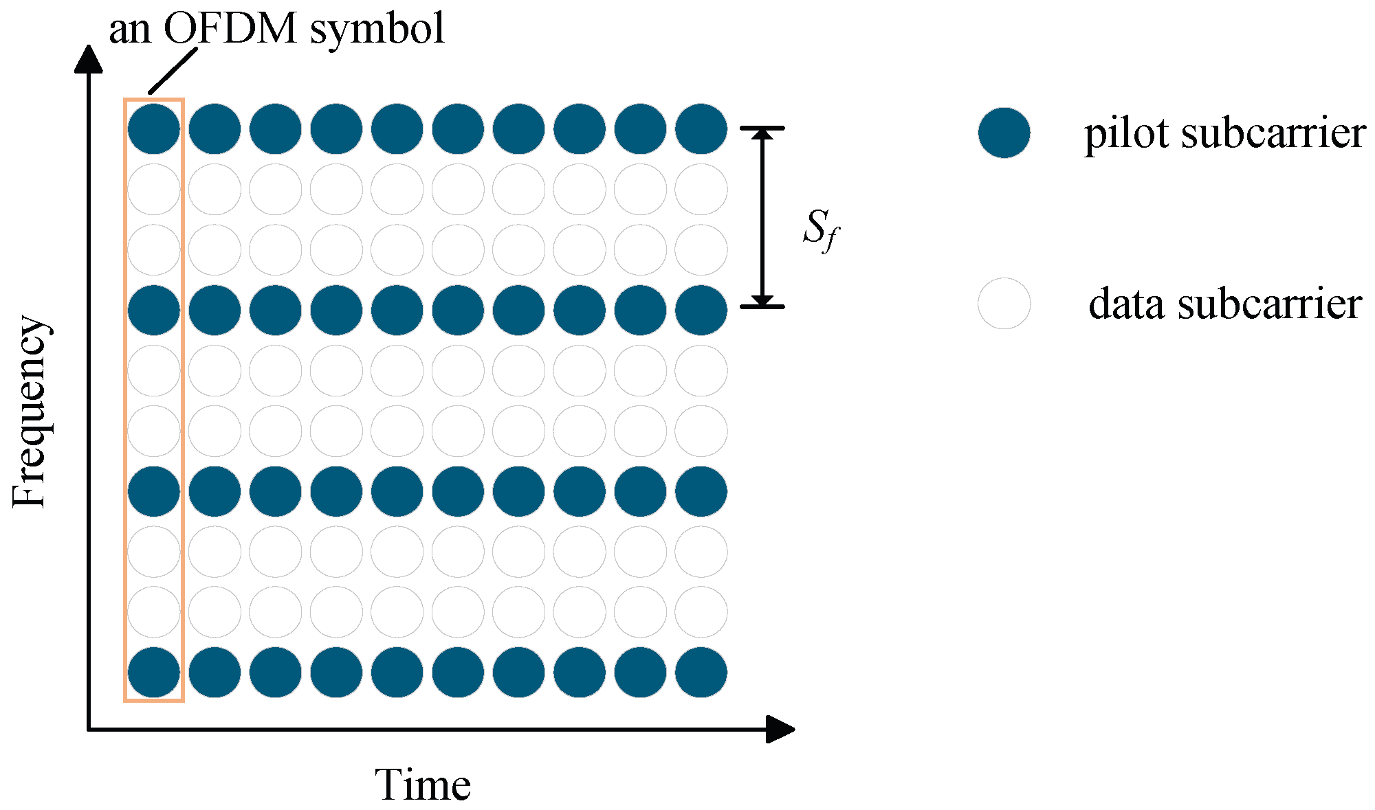
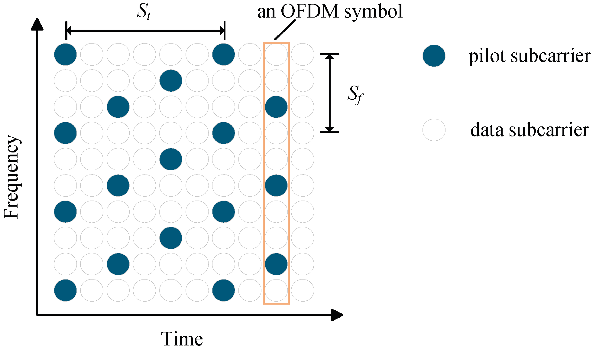
2.1.1. Pilot Arrangements
- Block-Type Pilot Arrangement
- Comb-Type Pilot Arrangement
- Lattice-Type Pilot Arrangement
2.1.2. LS Channel Estimation
2.1.3. MMSE Channel Estimation
2.1.4. LMMSE Channel Estimation
2.2. Blind Channel Estimation Method
2.2.1. Subspace-Based Blind Channel Estimation
2.2.2. HOS-Based Blind Channel Estimation
2.2.3. ML-Based Blind Channel Estimation
2.3. Semi-Blind Channel Estimation Method
2.3.1. Subspace-Based Semi-Blind Channel Estimation
2.3.2. EM-Based Semi-Blind Channel Estimation
3. Deep-Learning-Based Channel Estimation Methods
3.1. Overview of Neural Networks
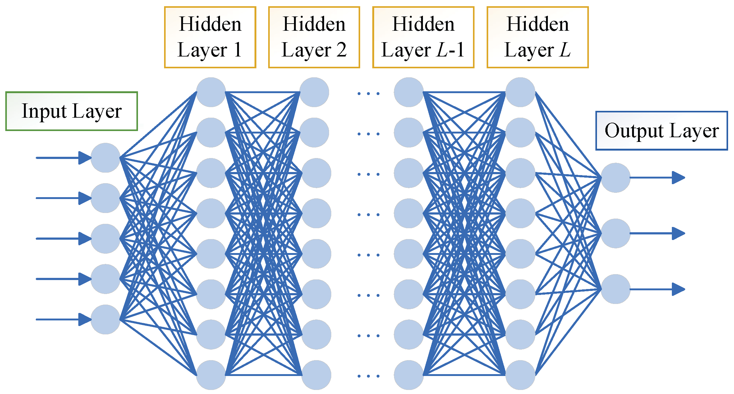
3.1.1. DNN
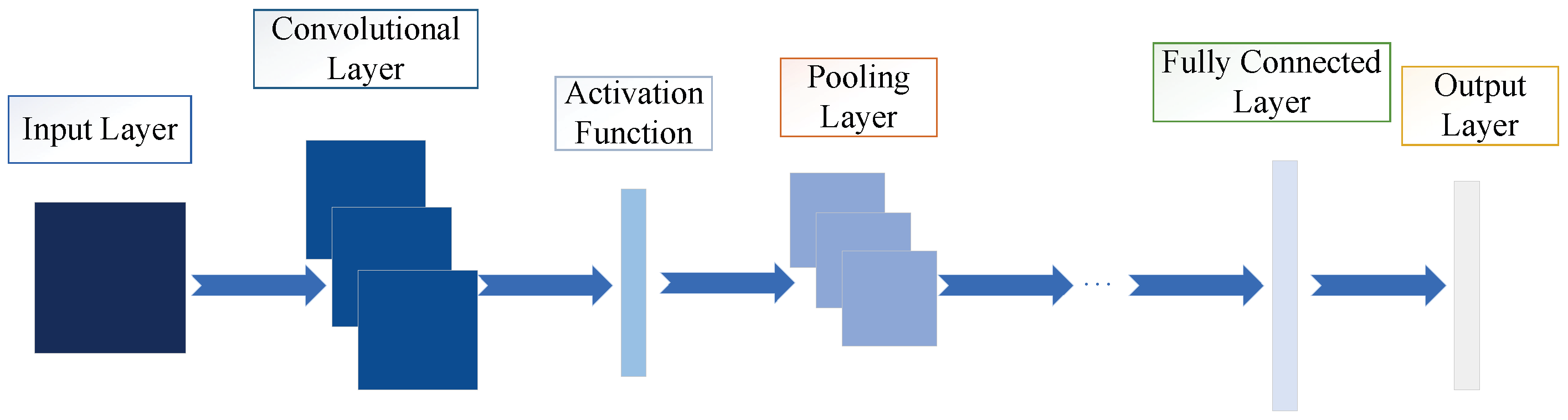
3.1.2. CNN
3.1.3. RNN
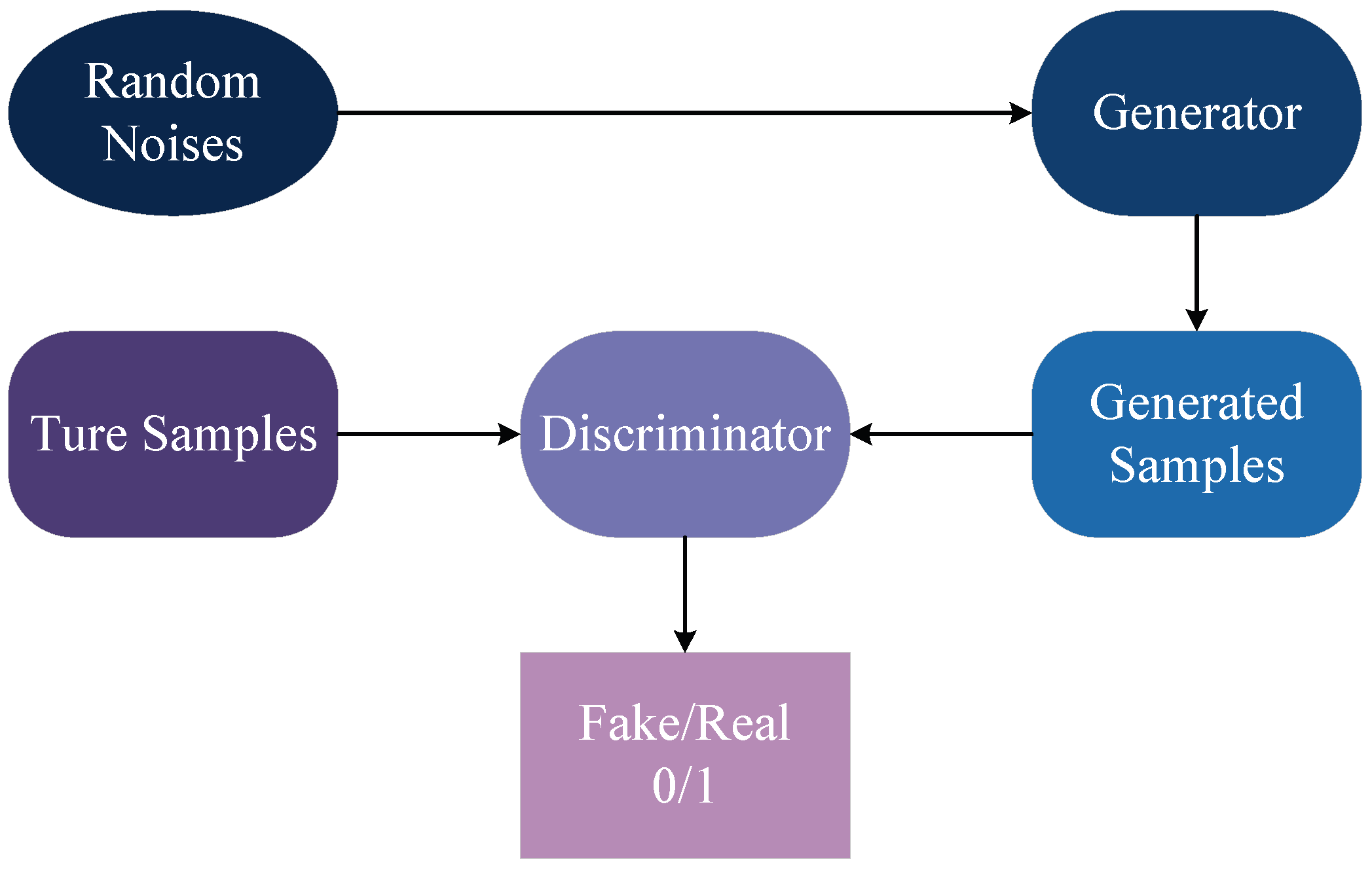
3.1.4. GAN
3.2. Toy Example of Deep Learning Application in Channel Estimation
3.3. Data-Driven Deep-Learning-Based Channel Estimation Methods
3.3.1. Application of DNN in Data-Driven Channel Estimation
3.3.2. Application of CNN in Data-Driven Channel Estimation
3.3.3. Application of RNN in Data-Driven Channel Estimation
3.3.4. Application of GAN in Data-Driven Channel Estimation
3.4. Model-Driven Deep-Learning-Based Channel Estimation Methods
3.4.1. Model-Driven Channel Estimation Combining LS Algorithm
3.4.2. Model-Driven Channel Estimation Combining OMP Algorithm
3.4.3. Model-Driven Channel Estimation Combining AMP Algorithm
4. Channel Estimation Based on Deep Learning for RIS-Aided Communication Systems
4.1. Application of Deep Learning in Channel Estimation for RIS-Aided Massive MIMO Systems
4.2. Application of Deep Learning in Channel Estimation for RIS-Aided mmWave Systems
4.3. Application of Deep Learning in Channel Estimation for RIS-Aided MU Systems
5. Challenges and Future Research Trends
5.1. Theoretical Exploration
5.2. Enhancing Estimation with Limited Data
5.3. Attention Mechanism in Noise Processing
5.4. Adaptation to Dynamic Environments
5.5. Channel Estimation for Other 6G Communication Scenarios
5.6. Lightweight Networks for Channel Estimation
6. Conclusions
Author Contributions
Funding
Data Availability Statement
Conflicts of Interest
References
- Henry, S.; Alsohaily, A.; Sousa, E.S. 5G is Real: Evaluating the Compliance of the 3GPP 5G New Radio System with the ITU IMT-2020 Requirements. IEEE Access 2020, 8, 42828–42840. [Google Scholar] [CrossRef]
- You, X.; Wang, C.X.; Huang, J.; Gao, X.; Zhang, Z.; Wang, M.; Huang, Y.; Zhang, C.; Jiang, Y.; Wang, J.; et al. Towards 6G wireless communication networks: Vision, enabling technologies, and new paradigm shifts. Sci. China Inf. Sci. 2021, 64, 110301. [Google Scholar] [CrossRef]
- Wang, C.X.; You, X.; Gao, X.; Zhu, X.; Li, Z.; Zhang, C.; Wang, H.; Huang, Y.; Chen, Y.; Haas, H.; et al. On the road to 6G: Visions, requirements, key technologies and testbeds. IEEE Commun. Surv. Tutor. 2023, 25, 905–974. [Google Scholar] [CrossRef]
- Cui, M.; Dai, L. Channel Estimation for Extremely Large-Scale MIMO: Far-Field or Near-Field? IEEE Trans. Commun. 2022, 70, 2663–2677. [Google Scholar] [CrossRef]
- Kolliboina, S.S.; Teja, S.; Giridhar, K. Non-Parametric Adaptive Thresholding for Channel Estimation of OTFS-Based 6G Communication Links. In Proceedings of the 2022 IEEE Globecom Workshops (GC Wkshps), Rio de Janeiro, Brazil, 4–8 December 2022; pp. 1561–1566. [Google Scholar] [CrossRef]
- Mao, Q.; Hu, F.; Hao, Q. Deep learning for intelligent wireless networks: A comprehensive survey. IEEE Commun. Surv. Tutor. 2018, 20, 2595–2621. [Google Scholar] [CrossRef]
- Qin, Z.; Ye, H.; Li, G.Y.; Juang, B.H.F. Deep learning in physical layer communications. IEEE Wirel. Commun. 2019, 26, 93–99. [Google Scholar] [CrossRef]
- Huang, H.; Guo, S.; Gui, G.; Yang, Z.; Zhang, J.; Sari, H.; Adachi, F. Deep Learning for Physical-Layer 5G Wireless Techniques: Opportunities, Challenges and Solutions. IEEE Wirel. Commun. 2020, 27, 214–222. [Google Scholar] [CrossRef]
- Ye, H.; Li, G.Y.; Juang, B.H. Power of Deep Learning for Channel Estimation and Signal Detection in OFDM Systems. IEEE Wirel. Commun. Lett. 2018, 7, 114–117. [Google Scholar] [CrossRef]
- Aboulfotouh, A.; De Oliveira, T.E.A.; Fadlullah, Z.M. Channel Estimation in Cellular Massive MIMO: A Data-Driven Approach. In Proceedings of the 2022 IEEE International Conference on Internet of Things and Intelligence Systems (IoTaIS), Bali, Indonesia, 24–26 November 2022; pp. 290–296. [Google Scholar] [CrossRef]
- Thakkar, K.; Goyal, A.; Bhattacharyya, B. Deep Learning and Channel Estimation. In Proceedings of the 2020 6th International Conference on Advanced Computing and Communication Systems (ICACCS), Coimbatore, India, 6–7 March 2020; pp. 745–751. [Google Scholar] [CrossRef]
- Gao, X.; Jin, S.; Wen, C.K.; Li, G.Y. ComNet: Combination of Deep Learning and Expert Knowledge in OFDM Receivers. IEEE Commun. Lett. 2018, 22, 2627–2630. [Google Scholar] [CrossRef]
- He, H.; Wen, C.K.; Jin, S.; Li, G.Y. Deep Learning-Based Channel Estimation for Beamspace mmWave Massive MIMO Systems. IEEE Wirel. Commun. Lett. 2018, 7, 852–855. [Google Scholar] [CrossRef]
- Zamanipour, M. A survey on deep-learning based techniques for modeling and estimation of massivemimo channels. arXiv 2019, arXiv:1910.03390. [Google Scholar]
- Boloursaz Mashhadi, M.; Gündüz, D. Deep learning for massive MIMO channel state acquisition and feedback. J. Indian Inst. Sci. 2020, 100, 369–382. [Google Scholar] [CrossRef] [PubMed]
- Peng, G.; Zhu, Z.; Liang, Y. Application of Deep Learning in Wireless Networks for Channel Estimation: A Survey. J. Phys. Conf. Ser. 2022, 2203, 012044. [Google Scholar] [CrossRef]
- Gizzini, A.K.; Chafii, M. A Survey on Deep Learning Based Channel Estimation in Doubly Dispersive Environments. IEEE Access 2022, 10, 70595–70619. [Google Scholar] [CrossRef]
- Vilas Boas, E.C.; e Silva, J.D.; de Figueiredo, F.A.; Mendes, L.L.; de Souza, R.A. Artificial intelligence for channel estimation in multicarrier systems for B5G/6G communications: A survey. EURASIP J. Wirel. Commun. Netw. 2022, 2022, 116. [Google Scholar] [CrossRef]
- Cui, T.J.; Qi, M.Q.; Wan, X.; Zhao, J.; Cheng, Q. Coding metamaterials, digital metamaterials and programmable metamaterials. Light. Sci. Appl. 2014, 3, e218. [Google Scholar] [CrossRef]
- Wei, X.; Shen, D.; Dai, L. Channel Estimation for RIS Assisted Wireless Communications—Part I: Fundamentals, Solutions, and Future Opportunities. IEEE Commun. Lett. 2021, 25, 1398–1402. [Google Scholar] [CrossRef]
- Oyerinde, O.O.; Mneney, S.H. Review of Channel Estimation for Wireless Communication Systems. IETE Tech. Rev. 2012, 29, 282–298. [Google Scholar] [CrossRef]
- Dong, X.; Lu, W.S.; Soong, A.C. Linear Interpolation in Pilot Symbol Assisted Channel Estimation for OFDM. IEEE Trans. Wirel. Commun. 2007, 6, 1910–1920. [Google Scholar] [CrossRef]
- Coleri, S.; Ergen, M.; Puri, A.; Bahai, A. Channel estimation techniques based on pilot arrangement in OFDM systems. IEEE Trans. Broadcast. 2002, 48, 223–229. [Google Scholar] [CrossRef]
- Dowler, A.; Doufexi, A.; Nix, A. Performance evaluation of channel estimation techniques for a mobile fourth generation wide area OFDM system. In Proceedings of the IEEE 56th Vehicular Technology Conference, Vancouver, BC, Canada, 24–28 September 2002; Volume 4, pp. 2036–2040. [Google Scholar] [CrossRef]
- Kwak, K.; Lee, S.; Kim, J.; Hong, D. A New DFT-Based Channel Estimation Approach for OFDM with Virtual Subcarriers by Leakage Estimation. IEEE Trans. Wirel. Commun. 2008, 7, 2004–2008. [Google Scholar] [CrossRef]
- Jeon, W.G.; Paik, K.H.; Cho, Y.S. An efficient channel estimation technique for OFDM systems with transmitter diversity. In Proceedings of the 11th IEEE International Symposium on Personal Indoor and Mobile Radio Communications. PIMRC 2000. Proceedings (Cat. No.00TH8525), London, UK, 18–21 September 2000; Volume 2, pp. 1246–1250. [Google Scholar] [CrossRef]
- Liu, Y.; Tan, Z.; Hu, H.; Cimini, L.J.; Li, G.Y. Channel Estimation for OFDM. IEEE Commun. Surv. Tutor. 2014, 16, 1891–1908. [Google Scholar] [CrossRef]
- Gong, Y.; Letaief, K. Low rank channel estimation for space-time coded wideband OFDM systems. In Proceedings of the IEEE 54th Vehicular Technology Conference. VTC Fall 2001. Proceedings (Cat. No.01CH37211), Atlantic City, NJ, USA, 7–11 October 2001; Volume 2, pp. 772–776. [Google Scholar] [CrossRef]
- Luo, Z.; Huang, D. General MMSE Channel Estimation for MIMO-OFDM Systems. In Proceedings of the 2008 IEEE 68th Vehicular Technology Conference, Calgary, AB, Canada, 21–24 September 2008; pp. 1–5. [Google Scholar] [CrossRef]
- Hung, K.C.; Lin, D.W. Pilot-Based LMMSE Channel Estimation for OFDM Systems With Power–Delay Profile Approximation. IEEE Trans. Veh. Technol. 2010, 59, 150–159. [Google Scholar] [CrossRef]
- Rossi, P.S.; Müller, R.R.; Edfors, O. Linear MMSE estimation of time–frequency variant channels for MIMO-OFDM systems. Signal Process. 2011, 91, 1157–1167. [Google Scholar] [CrossRef]
- Yu, J.L.; Zhang, B.; Chen, P.T. Blind and semi-blind channel estimation with fast convergence for MIMO-OFDM systems. Signal Process. 2014, 95, 1–9. [Google Scholar] [CrossRef]
- Shin, C.; Heath, R.W.; Powers, E.J. Blind channel estimation for MIMO-OFDM systems. IEEE Trans. Veh. Technol. 2007, 56, 670–685. [Google Scholar] [CrossRef]
- Kang, W.; Champagne, B. Subspace-based blind channel estimation: Generalization and performance analysis. IEEE Trans. Signal Process. 2005, 53, 1151–1162. [Google Scholar] [CrossRef]
- Tu, C.C.; Champagne, B. Subspace-Based Blind Channel Estimation for MIMO-OFDM Systems With Reduced Time Averaging. IEEE Trans. Veh. Technol. 2010, 59, 1539–1544. [Google Scholar] [CrossRef]
- Acar, T.; Petropulu, A. Blind MIMO system identification using PARAFAC decomposition of an output HOS-based tensor. In Proceedings of the The Thrity-Seventh Asilomar Conference on Signals, Systems & Computers, Pacific Grove, CA, USA, 9–12 November 2003; Volume 1, pp. 1080–1084. [Google Scholar] [CrossRef]
- Choqueuse, V.; Mansour, A.; Burel, G.; Collin, L.; Yao, K. Blind Channel Estimation for STBC Systems Using Higher-Order Statistics. IEEE Trans. Wirel. Commun. 2011, 10, 495–505. [Google Scholar] [CrossRef]
- Cirpan, H.; Tsatsanis, M. Maximum likelihood blind channel estimation in the presence of Doppler shifts. IEEE Trans. Signal Process. 1999, 47, 1559–1569. [Google Scholar] [CrossRef]
- Necker, M.; Stuber, G. Totally blind channel estimation for OFDM over fast varying mobile channels. In Proceedings of the 2002 IEEE International Conference on Communications. Conference Proceedings. ICC 2002 (Cat. No.02CH37333), New York, NY, USA, 28 April–2 May 2002; Volume 1, pp. 421–425. [Google Scholar] [CrossRef]
- Wu, C.Y.; Huang, W.J.; Chung, W.H. Low-Complexity Semiblind Channel Estimation in Massive MU-MIMO Systems. IEEE Trans. Wirel. Commun. 2017, 16, 6279–6290. [Google Scholar] [CrossRef]
- Kawasaki, H.; Matsumura, T. Semi-Blind Channel Estimation by Subspace Method for Orthogonal Precoded OFDM Systems. In Proceedings of the 2022 IEEE 33rd Annual International Symposium on Personal, Indoor and Mobile Radio Communications (PIMRC), Kyoto, Japan, 12–15 September 2022; pp. 451–456. [Google Scholar] [CrossRef]
- Moon, T. The expectation-maximization algorithm. IEEE Signal Process. Mag. 1996, 13, 47–60. [Google Scholar] [CrossRef]
- Obradovic, D.; Na, C.; Scheiterer, R.L.; Szabo, A. EM-based semi-blind channel estimation method for MIMO-OFDM communication systems. Neurocomputing 2008, 71, 2388–2398. [Google Scholar] [CrossRef]
- Nayebi, E.; Rao, B.D. Semi-blind Channel Estimation for Multiuser Massive MIMO Systems. IEEE Trans. Signal Process. 2018, 66, 540–553. [Google Scholar] [CrossRef]
- O’Shea, T.; Hoydis, J. An Introduction to Deep Learning for the Physical Layer. IEEE Trans. Cogn. Commun. Netw. 2017, 3, 563–575. [Google Scholar] [CrossRef]
- Khalid, W.; Yu, H.; Ali, R.; Ullah, R. Advanced physical-layer technologies for beyond 5G wireless communication networks. Sensors 2021, 21, 3197. [Google Scholar] [CrossRef]
- Kim, W.; Ahn, Y.; Kim, J.; Shim, B. Towards deep learning-aided wireless channel estimation and channel state information feedback for 6G. J. Commun. Netw. 2023, 25, 61–75. [Google Scholar] [CrossRef]
- LeCun, Y.; Boser, B.; Denker, J.S.; Henderson, D.; Howard, R.E.; Hubbard, W.; Jackel, L.D. Backpropagation Applied to Handwritten Zip Code Recognition. Neural Comput. 1989, 1, 541–551. [Google Scholar] [CrossRef]
- Sak, H.; Senior, A.; Beaufays, F. Long short-term memory based recurrent neural network architectures for large vocabulary speech recognition. arXiv 2014, arXiv:1402.1128. [Google Scholar] [CrossRef]
- Mirza, M.; Osindero, S. Conditional generative adversarial nets. arXiv 2014, arXiv:1411.1784. [Google Scholar] [CrossRef]
- Ma, X.; Gao, Z. Data-Driven Deep Learning to Design Pilot and Channel Estimator for Massive MIMO. IEEE Trans. Veh. Technol. 2020, 69, 5677–5682. [Google Scholar] [CrossRef]
- Ge, L.; Guo, Y.; Zhang, Y.; Chen, G.; Wang, J.; Dai, B.; Li, M.; Jiang, T. Deep Neural Network Based Channel Estimation for Massive MIMO-OFDM Systems With Imperfect Channel State Information. IEEE Syst. J. 2022, 16, 4675–4685. [Google Scholar] [CrossRef]
- Zheng, X.; Lau, V.K.N. Online Deep Neural Networks for MmWave Massive MIMO Channel Estimation with Arbitrary Array Geometry. IEEE Trans. Signal Process. 2021, 69, 2010–2025. [Google Scholar] [CrossRef]
- Zhang, Y.; Wang, H.; Li, C.; Chen, X.; Meriaudeau, F. On the performance of deep neural network aided channel estimation for underwater acoustic OFDM communications. Ocean Eng. 2022, 259, 111518. [Google Scholar] [CrossRef]
- Li, X.; Han, Z.; Yu, H.; Yan, L.; Han, S. Deep Learning for OFDM Channel Estimation in Impulsive Noise Environments. Wirel. Pers. Commun. 2022, 125, 2947–2964. [Google Scholar] [CrossRef]
- Mehlführer, C.; Colom Ikuno, J.; Šimko, M.; Schwarz, S.; Wrulich, M.; Rupp, M. The Vienna LTE simulators-Enabling reproducibility in wireless communications research. EURASIP J. Adv. Signal Process. 2011, 2011, 29. [Google Scholar] [CrossRef]
- Soltani, M.; Pourahmadi, V.; Mirzaei, A.; Sheikhzadeh, H. Deep Learning-Based Channel Estimation. IEEE Commun. Lett. 2019, 23, 652–655. [Google Scholar] [CrossRef]
- Li, L.; Chen, H.; Chang, H.H.; Liu, L. Deep Residual Learning Meets OFDM Channel Estimation. IEEE Wirel. Commun. Lett. 2020, 9, 615–618. [Google Scholar] [CrossRef]
- Pradhan, A.; Das, S.; Dayalan, D. A Two-Stage CNN Based Channel Estimation for OFDM System. In Proceedings of the 2021 Advanced Communication Technologies and Signal Processing (ACTS), Rourkela, India, 15–17 December 2021; pp. 1–4. [Google Scholar] [CrossRef]
- Li, J.; Peng, Q. Lightweight Channel Estimation Networks for OFDM Systems. IEEE Wirel. Commun. Lett. 2022, 11, 2066–2070. [Google Scholar] [CrossRef]
- Zhao, J.; Wu, Y.; Zhang, Q.; Liao, J. Two-Stage Channel Estimation for mmWave Massive MIMO Systems Based on ResNet-UNet. IEEE Syst. J. 2023, 17, 4291–4300. [Google Scholar] [CrossRef]
- Rahman, M.H.; Chowdhury, M.Z.; Utama, I.B.K.Y.; Jang, Y.M. Channel Estimation for Indoor Massive MIMO Visible Light Communication with Deep Residual Convolutional Blind Denoising Network. IEEE Trans. Cogn. Commun. Netw. 2023, 9, 683–694. [Google Scholar] [CrossRef]
- Gizzini, A.K.; Chafii, M. Deep Learning Based Channel Estimation in High Mobility Communications Using Bi-RNN Networks. arXiv 2023, arXiv:2305.00208. [Google Scholar] [CrossRef]
- Ali, M.H.E.; Taha, I.B. Channel state information estimation for 5G wireless communication systems: Recurrent neural networks approach. PeerJ Comput. Sci. 2021, 7, e682. [Google Scholar] [CrossRef]
- Essai Ali, M.H.; Rabeh, M.L.; Hekal, S.; Abbas, A.N. Deep Learning Gated Recurrent Neural Network-Based Channel State Estimator for OFDM Wireless Communication Systems. IEEE Access 2022, 10, 69312–69322. [Google Scholar] [CrossRef]
- Helmy, I.; Tarafder, P.; Choi, W. LSTM-GRU Model-Based Channel Prediction for One-Bit Massive MIMO System. IEEE Trans. Veh. Technol. 2023, 72, 11053–11057. [Google Scholar] [CrossRef]
- Zhao, S.; Fang, Y.; Qiu, L. Deep Learning-Based channel estimation with SRGAN in OFDM Systems. In Proceedings of the 2021 IEEE Wireless Communications and Networking Conference (WCNC), Nanjing, China, 29 March–1 April 2021; pp. 1–6. [Google Scholar] [CrossRef]
- Dong, Y.; Wang, H.; Yao, Y.D. Channel Estimation for One-Bit Multiuser Massive MIMO Using Conditional GAN. IEEE Commun. Lett. 2021, 25, 854–858. [Google Scholar] [CrossRef]
- Zhang, Q.; Dong, H.; Zhao, J. Channel Estimation for High-Speed Railway Wireless Communications: A Generative Adversarial Network Approach. Electronics 2023, 12, 1752. [Google Scholar] [CrossRef]
- Kang, X.F.; Liu, Z.H.; Yao, M. Deep learning for joint pilot design and channel estimation in MIMO-OFDM systems. Sensors 2022, 22, 4188. [Google Scholar] [CrossRef]
- Jiang, P.; Wen, C.K.; Jin, S.; Li, G.Y. Dual CNN-Based Channel Estimation for MIMO-OFDM Systems. IEEE Trans. Commun. 2021, 69, 5859–5872. [Google Scholar] [CrossRef]
- Haq, S.A.U.; Gizzini, A.K.; Shrey, S.; Darak, S.J.; Saurabh, S.; Chafii, M. Deep Neural Network Augmented Wireless Channel Estimation for Preamble-Based OFDM PHY on Zynq System on Chip. IEEE Trans. Very Large Scale Integr. (VLSI) Syst. 2023, 31, 1026–1038. [Google Scholar] [CrossRef]
- Li, Y.; Bian, X.; Li, M. Denoising Generalization Performance of Channel Estimation in Multipath Time-Varying OFDM Systems. Sensors 2023, 23, 3102. [Google Scholar] [CrossRef] [PubMed]
- Hu, Z.; Chen, Y.; Han, C. PRINCE: A Pruned AMP Integrated Deep CNN Method for Efficient Channel Estimation of Millimeter-wave and Terahertz Ultra-Massive MIMO Systems. IEEE Trans. Wirel. Commun. 2023, 22, 8066–8079. [Google Scholar] [CrossRef]
- Li, Q.; Gong, Y.; Meng, F.; Li, Z.; Miao, L.; Xu, Z. Residual Learning based Channel Estimation for OTFS system. In Proceedings of the 2022 IEEE/CIC International Conference on Communications in China (ICCC Workshops), Foshan, China, 11–13 August 2022; pp. 275–280. [Google Scholar] [CrossRef]
- Tong, W.; Xu, W.; Wang, F.; Shang, J.; Pan, M.; Lin, J. Deep Learning Compressed Sensing-Based Beamspace Channel Estimation in mmWave Massive MIMO Systems. IEEE Wirel. Commun. Lett. 2022, 11, 1935–1939. [Google Scholar] [CrossRef]
- Nayir, H.; Karakoca, E.; Görçin, A.; Qaraqe, K. Hybrid-Field Channel Estimation for Massive MIMO Systems based on OMP Cascaded Convolutional Autoencoder. In Proceedings of the 2022 IEEE 96th Vehicular Technology Conference (VTC2022-Fall), London, UK, 26–29 September 2022; pp. 1–6. [Google Scholar] [CrossRef]
- Donoho, D.L.; Maleki, A.; Montanari, A. Message passing algorithms for compressed sensing: I. motivation and construction. In Proceedings of the 2010 IEEE Information Theory Workshop on Information Theory (ITW 2010, Cairo), Cairo, Egypt, 6–8 January 2010; pp. 1–5. [Google Scholar] [CrossRef]
- Wei, X.; Hu, C.; Dai, L. Deep Learning for Beamspace Channel Estimation in Millimeter-Wave Massive MIMO Systems. IEEE Trans. Commun. 2021, 69, 182–193. [Google Scholar] [CrossRef]
- Pu, X.; Liu, Y.; Song, M.; Chen, Q. Orthogonal Time Frequency Space Channel Estimation Based on Model-driven Deep Learning. J. Electron. Inf. Technol. 2023, 45, 1–8. [Google Scholar] [CrossRef]
- Wang, P.; Li, J.; Liu, X.; Wang, P. Multi-Stage Training Optimization for Pilot Compression and Channel Estimation in Massive MIMO Systems Under Quasi-Sparse Channel Environment. IEEE Commun. Lett. 2022, 26, 3059–3063. [Google Scholar] [CrossRef]
- Yuan, X.; Zhang, Y.J.A.; Shi, Y.; Yan, W.; Liu, H. Reconfigurable-Intelligent-Surface Empowered Wireless Communications: Challenges and Opportunities. IEEE Wirel. Commun. 2021, 28, 136–143. [Google Scholar] [CrossRef]
- Tang, W.; Chen, X.; Chen, M.Z.; Dai, J.Y.; Han, Y.; Jin, S.; Cheng, Q.; Li, G.Y.; Cui, T.J. On Channel Reciprocity in Reconfigurable Intelligent Surface Assisted Wireless Networks. IEEE Wirel. Commun. 2021, 28, 94–101. [Google Scholar] [CrossRef]
- Mao, Z.; Liu, X.; Peng, M. Channel Estimation for Intelligent Reflecting Surface Assisted Massive MIMO Systems—A Deep Learning Approach. IEEE Commun. Lett. 2022, 26, 798–802. [Google Scholar] [CrossRef]
- Xie, W.; Xiao, J.; Zhu, P.; Yu, C.; Yang, L. Deep Compressed Sensing-Based Cascaded Channel Estimation for RIS-Aided Communication Systems. IEEE Wirel. Commun. Lett. 2022, 11, 846–850. [Google Scholar] [CrossRef]
- Liu, M.; Li, X.; Ning, B.; Huang, C.; Sun, S.; Yuen, C. Deep Learning-Based Channel Estimation for Double-RIS Aided Massive MIMO System. IEEE Wirel. Commun. Lett. 2023, 12, 70–74. [Google Scholar] [CrossRef]
- Liu, S.; Gao, Z.; Zhang, J.; Renzo, M.D.; Alouini, M.S. Deep Denoising Neural Network Assisted Compressive Channel Estimation for mmWave Intelligent Reflecting Surfaces. IEEE Trans. Veh. Technol. 2020, 69, 9223–9228. [Google Scholar] [CrossRef]
- Shtaiwi, E.; Zhang, H.; Abdelhadi, A.; Han, Z. RIS-Assisted mmWave Channel Estimation Using Convolutional Neural Networks. In Proceedings of the 2021 IEEE Wireless Communications and Networking Conference Workshops (WCNCW), Nanjing, China, 29 March 2021; pp. 1–6. [Google Scholar] [CrossRef]
- Jin, Y.; Zhang, J.; Zhang, X.; Xiao, H.; Ai, B.; Ng, D.W.K. Channel Estimation for Semi-Passive Reconfigurable Intelligent Surfaces With Enhanced Deep Residual Networks. IEEE Trans. Veh. Technol. 2021, 70, 11083–11088. [Google Scholar] [CrossRef]
- Feng, H.; Zhao, Y. mmWave RIS-Assisted SIMO Channel Estimation Based on Global Attention Residual Network. IEEE Wirel. Commun. Lett. 2023, 12, 1179–1183. [Google Scholar] [CrossRef]
- Abdallah, A.; Celik, A.; Mansour, M.M.; Eltawil, A.M. RIS-Aided mmWave MIMO Channel Estimation Using Deep Learning and Compressive Sensing. IEEE Trans. Wirel. Commun. 2023, 22, 3503–3521. [Google Scholar] [CrossRef]
- Ginige, N.; Shashika Manosha, K.B.; Rajatheva, N.; Latva-aho, M. Untrained DNN for Channel Estimation of RIS-Assisted Multi-User OFDM System with Hardware Impairments. In Proceedings of the 2021 IEEE 32nd Annual International Symposium on Personal, Indoor and Mobile Radio Communications (PIMRC), Helsinki, Finland, 13–16 September 2021; pp. 561–566. [Google Scholar] [CrossRef]
- Liu, C.; Liu, X.; Ng, D.W.K.; Yuan, J. Deep Residual Learning for Channel Estimation in Intelligent Reflecting Surface-Assisted Multi-User Communications. IEEE Trans. Wirel. Commun. 2022, 21, 898–912. [Google Scholar] [CrossRef]
- Shen, W.; Qin, Z.; Nallanathan, A. Deep Learning for Super-Resolution Channel Estimation in Reconfigurable Intelligent Surface Aided Systems. IEEE Trans. Commun. 2023, 71, 1491–1503. [Google Scholar] [CrossRef]
- Li, T.; Yang, Y.; Lee, J.; Qin, X.; Huang, J.; He, G. DCSaNet: Dilated Convolution and Self-Attention-Based Neural Network for Channel Estimation in IRS-Aided Multi-User Communication System. IEEE Wirel. Commun. Lett. 2023, 12, 1139–1143. [Google Scholar] [CrossRef]
- Dai, L.; Jiao, R.; Adachi, F.; Poor, H.V.; Hanzo, L. Deep Learning for Wireless Communications: An Emerging Interdisciplinary Paradigm. IEEE Wirel. Commun. 2020, 27, 133–139. [Google Scholar] [CrossRef]
- Qing, C.; Dong, L.; Wang, L.; Ling, G.; Wang, J. Transfer learning-based channel estimation in orthogonal frequency division multiplexing systems using data-nulling superimposed pilots. PLoS ONE 2022, 17, e0268952. [Google Scholar] [CrossRef]
- Kim, D.; Park, S.; Kang, J.; Kang, J. Block-Fading Non-Stationary Channel Estimation for MIMO-OFDM Systems via Meta-Learning. IEEE Commun. Lett. 2022, 26, 2924–2928. [Google Scholar] [CrossRef]
- Gao, W.; Zhang, W.; Liu, L.; Yang, M. Deep Residual Learning with Attention Mechanism for OFDM Channel Estimation. IEEE Wirel. Commun. Lett. 2022; early access. [Google Scholar] [CrossRef]
- Niu, Z.; Zhong, G.; Yu, H. A review on the attention mechanism of deep learning. Neurocomputing 2021, 452, 48–62. [Google Scholar] [CrossRef]
- Serghiou, D.; Khalily, M.; Brown, T.W.C.; Tafazolli, R. Terahertz Channel Propagation Phenomena, Measurement Techniques and Modeling for 6G Wireless Communication Applications: A Survey, Open Challenges and Future Research Directions. IEEE Commun. Surv. Tutor. 2022, 24, 1957–1996. [Google Scholar] [CrossRef]
- Sejan, M.A.S.; Rahman, M.H.; Aziz, M.A.; Kim, D.S.; You, Y.H.; Song, H.K. A Comprehensive Survey on MIMO Visible Light Communication: Current Research, Machine Learning and Future Trends. Sensors 2023, 23, 739. [Google Scholar] [CrossRef]


| Article | Year | Main Contribution |
|---|---|---|
| [14] | 2019 | It groups the challenges (such as feedback overhead) in massive MIMO channel modeling and estimation according to four technical details, followed by a discussion of each group’s relevant deep-learning-based solutions. |
| [15] | 2020 | It outlines how to use deep learning to enhance the performance of massive MIMO channel estimation while reducing training overhead, followed by introducing some data-driven methods. |
| [16] | 2022 | It reviews various deep learning models used for channel estimation. Subsequently, it introduces the channel estimation methods that use deep learning in different systems. |
| [17] | 2022 | It overviews recent channel estimation methods using deep learning in doubly-dispersive channels and conducts experimental comparisons and simulation analyses under various frame sizes, modulation orders, and mobility scenarios. |
| [18] | 2022 | It provides a comprehensive summary of artificial intelligence-assisted channel estimation methods in multicarrier systems, which include machine learning and neural networks. |
| This review | 2023 | This paper discusses data-driven channel estimation methods based on different fundamental neural networks. It also introduces model-driven methods, which are categorized according to various benchmark algorithms. Additionally, this paper overviews recent studies on deep-learning-based channel estimation in RIS-aided communication systems. |
| Methods | Advantages | Disadvantages |
|---|---|---|
| Pilot-based channel estimation | Low computational complexity | Waste of spectrum resources |
| Easy to implement | Low transmission efficiency | |
| Pilot can improve estimation performance | ||
| Blind channel estimation | Efficient use of spectrum resources | High computational complexity |
| Able to adaptively track the dynamic changes of the channel | Slow convergence speed | |
| Presence of phase ambiguity | ||
| Long observation time | ||
| Semi-blind channel estimation | Relatively high bandwidth efficiency | Relatively large amount of calculation |
| Able to solve phase ambiguity | Relatively difficult to implement | |
| Relatively fast convergence speed |
| Reference | Model | Input | Output | Compared with | Performance | Complexity |
|---|---|---|---|---|---|---|
| Ma et al. [51] | DNN | Original channel | Estimated channel | SOMP algorithm | Has better NMSE performance and can reduce pilot overhead | |
| Ge et al. [52] | DNN | Data subcarrier position index | Channel estimation of data subcarriers | LS algorithm | Has better NMSE and BER performance | \ |
| Zheng et al. [53] | DNN | Received signals and pilot symbols | Estimated channel | GOMP, MMSE, and burst LASSO algorithms | The NMSE performance is close to the GOMP and the burst LASSO algorithms while exceeding the MMSE algorithm | CPU time = 0.338 ms |
| Zhang et al. [54] | DNN | Received OFDM symbols and transmitted pilot symbols | Estimated channel | LS and MMSE algorithms | The BER performance is close to the MMSE algorithm, over 40% better than the LS algorithm | Parameters = 267.168 K, CPU time = 2.995 ms |
| Li et al. [55] | DAE-DNN | Noisy received signal | Estimated CSI | LS, OMP, MMSE algorithms, and DNN | Outperforms other methods in terms of BER and the MSE in impulse noise environments | \ |
| Soltani et al. [57] | ChannelNet (SRCNN + DNCNN) | Estimated channel at pilot positions | Estimated whole channel | Ideal MMSE and ideal ALMMSE algorithms | At SNR below 20 dB, the MSE performance is superior to the ideal MMSE algorithm but inferior to the ideal ALMMSE algorithm | Floating-point operations per second (FLOPs) = 1533.583 M, parameters = 130.754 K, predict time = 4.422 ms |
| Li et al. [58] | ReEsNet | Estimated channel at pilot positions | Estimated whole channel | LS, MMSE algorithms, and ChannelNet | The MSE performance is superior to the LS algorithm and the ChannelNet, comparable to the LMMSE algorithm | FLOPs = 5.875 M, parameters = 23.554 K, predict time = 1.737 ms |
| Pradhan et al. [59] | CENet (SRCNN + CBDNet) | Estimated channel at pilot positions | Estimated whole channel | Ideal MMSE algorithm and ChannelNet | The MSE performance is superior to the ChannelNet but inferior to the ideal MMSE algorithm | \ |
| Li et al. [60] | LCET (LFEC + LAT) | Estimated channel at pilot positions | Estimated whole channel | LS, LMMSE algorithms, ChannelNet, ReEsNet, and SRGAN | The MSE and the BER performance are superior to the LS algorithm and other deep learning networks and approach the LMMSE algorithm in multi-pilot scenarios | FLOPs = 19.316 M, parameters = 21.970 K, predict time = 5.439 ms |
| Zhao et al. [61] | ResNet-UNet | Noisy pilot sequences | Estimated channel | LS, MMSE algorithms, and deep CNN | Has the best NMSE performance and exhibits strong robustness in noisy environments | \ |
| Rahman et al. [62] | ResCBDNet | Noisy channel matrix | Estimated channel | DnCNN and FFDNet | The NMSE and the PSNR performance are significantly superior to the DnCNN and the FFDnet | Parameters = 536 K, inference time = 0.119 s |
| Gizzini et al. [63] | Bi-RNN | Estimated channel at pilot symbols | Estimated whole channel | 2D-LMMSE algorithm, ChannelNet, and Bi-LSTM | The BER performance is superior to the ChannelNet and the Bi-LSTM and is slightly inferior to the 2D-LMMSE algorithm | |
| Essai Ali et al. [64] | Bi-LSTM | Transmitted signal sequence | Prediction matrix of features extracted from the input sequence | LS, MMSE algorithms, and LSTM | With limited pilots, the SER performance is superior to all three | \ |
| Essai Ali et al. [65] | GRU | Received signals | Transmitted signals | LS, MMSE algorithms, DNN, and ReEsNet | With limited pilots, the SER performance is superior to other methods | \ |
| Helmy et al. [66] | LSTM-GRU | Received signals | Estimated channel | CNN and CGAN | Has the best NMSE performance | Computation time = 23.34 ms |
| Zhao et al. [67] | SRGAN | Estimated channel at pilot positions | Estimated whole channel | LS, LMMSE algorithms, and ReESNet | At low SNR, it provides the best MSE performance; while at high SNR, it is only slightly inferior to the LMMSE algorithm | FLOPs = 48.590 M, parameters = 24.102 K, predict time = 3.464 ms |
| Dong et al. [68] | CGAN | Received signals and pilot sequences | Estimated channel | U-Net and CNN | Has the best NMSE performance | Computation time = 25.88 ms |
| Zhang et al. [69] | N2N-CGAN | Noisy pilot sequences | Estimated channel | LS, MMSE algorithms, and CGAN | In terms of MSE, it is superior to the LS algorithm and CGAN and only slightly inferior to the MMSE algorithm at high SNR | |
| Kang et al. [70] | CAGAN (concrete AE + CGAN) | Noisy channel | Estimated channel | LS, MMSE algorithms, and ChannelNet | Outperforms the LS algorithm in terms of MSE and, under high SNR conditions, approaches the ideal MMSE algorithm, surpassing the ChannelNet | FLOPs = 548 K, parameters = 275 K |
| Reference | Deep Learning Model | Input | Output | Compared with | Performance | Complexity |
|---|---|---|---|---|---|---|
| Jiang et al. [71] | Dual CNN (SFCNN + ADCNN) | LS rough channel estimation result | Accurate channel estimation result | LMMSE, robust LMMSE (RLMMSE) algorithms, SFCNN, and ADCNN | The NMSE performance surpasses the RLMMSE algorithm, the SFCNN, and the ADCNN, while it is comparable to the LMMSE algorithm | FLOPs = 3.7 M, parameters = 1764 |
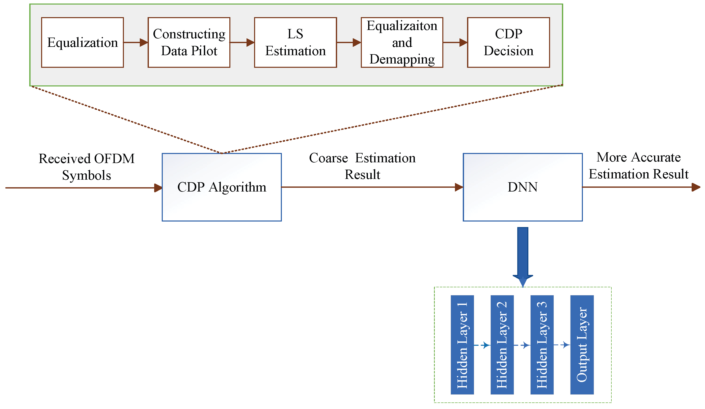
| Haq et al. [72] | DNN | LS rough channel estimation result | Accurate channel estimation result | LS and MMSE algorithms | Has the best NMSE and BER performances on SoC, the resource utilization is lower than the MMSE algorithm but higher than the LS algorithm | Execution time = 0.0179 ms, SoC power = 2.849 W |
| Li et al. [73] | NDR-Net (NLE + DnCNN + residual learning) | LS rough channel estimation result | Accurate channel estimation result | LS, MMSE algorithms, and DnCNN | Has a better MSE performance when the SNR is mismatched, with nearly 5–7 dB of gain compared to the MMSE algorithm | Parameters = 1231 K, FLOPs = 67 K |
| Li et al. [75] | ResNet | OMP rough channel estimation result | Accurate channel estimation result | OMP algorithm | Significantly superior to the OMP algorithm in terms of NMSE, especially when the frame size is 128 × 16, and the NMSE is 0.00173, the gain is close to 6dB | \ |
| Tong et al. [76] | SE-ResNet | Coarsely estimated AoAs/AoDs | Finely estimated AoAs/AoDs | SW-OMP, NOMP algorithms, and CENN | Has better NMSE performance even with low SNR and fewer training frames | |
| Nayir et al. [77] | CAE | OMP rough channel estimation result | Accurate channel estimation result | OMP and MMSE algorithms | Performs best in terms of NMSE, even at low SNR | \ |
| Wei et al. [79] | GM-LAMP | Measurement signal vector and beam selection matrix | Estimated channel | OMP, AMP and LAMP algorithms | Achieves better NMSE performance with lower pilot overhead | |
| Pu et al. [80] | LDAMP | Received signal vector and transmitted signal matrix | Estimated channel | OMP, AMP algorithms, and ResNet | Has the best NMSE performance, with the NMSE already less than in the low SNR scenario with an SNR of 2dB | |
| Wang et al. [81] | DNN | Original channel | Estimated channel | AMP, LAMP, and LDAMP algorithms | The NMSE performance outperforms the AMP and the LAMP algorithms; it outperforms the LDAMP algorithm when the SNR is above 8 dB | \ |
| Characteristics | Data-Driven Approach | Model-Driven Approach | |
|---|---|---|---|
| Advantages | Self-learning/automatic feature extraction | ✓ | |
| High accuracy | ✓ (With sufficient training data) | ✓ (When the model is well designed) | |
| Utilization of prior knowledge | ✓ | ||
| Interpretability | ✓ | ||
| Disadvantages | Large data requirements | ✓ | |
| Risk of overfitting | ✓ | ||
| High computational complexity | ✓ | ||
| Inflexibility | ✓ | ||
| Reference | System | RIS Architecture | Deep Learning Model | Input | Output | Complexity |
|---|---|---|---|---|---|---|
| Mao et al. [84] | RIS-aided massive MIMO | Entirely passive | ResNet | OMP rough channel estimation result | Accurate channel estimation result | |
| Xie et al. [85] | RIS-aided massive MIMO | Entirely passive | ResU-Net | Received pilot signal | Estimated channel | CPU time = 95.7 ms, GPU time = 4.27 ms |
| Liu et al. [86] | Double-RIS-aided massive MIMO | Entirely passive | SC-attention network | LS rough channel estimation result | Accurate channel estimation result | \ |
| Shtaiwi et al. [88] | RIS-aided mmWave MIMO | Entirely passive | STS-CNN | Partial CSI | Entire CSI | \ |
| Jin et al. [89] | RIS-aided mmWave massive MIMO | Semi-passive | EDSR + MDSR | Partial CSI | Entire CSI | EDSR: average running time = 7.8 ms MDSR: average running time = 7.5 ms |
| Feng et al. [90] | RIS-aided mmWave SIMO | Entirely passive | GARN (ResNet + global attention) | Grouped LS channel estimation matrix | Reconstructed complete channel matrix | Parameters = 2.061 M, FLOPs = 1.807 G |
| Abdallah et al. [91] | RIS-aided mmWave MIMO | Entirely passive | DnCNN | Received pilot signal | Residual noise | |
| Ginige et al. [92] | RIS-aided MU SIMO-OFDM | Entirely passive | DNN | LS rough channel estimation result | Accurate channel estimation result | \ |
| Liu et al. [93] | RIS-aided MUC | Entirely passive | CDRN (CNN + DRN) | Noisy channel matrix | Denoised channel matrix | computation time = 2.66 ms |
| Shen et al. [94] | RIS-aided MU MIMO-OFDM | Entirely passive | SRDnNet (SRCNN + DnCNN) | Estimated channel at pilot positions | Estimated whole channel | Predict time = 1.61 × s |
| Li et al. [95] | RIS-aided MUC | Entirely passive | DCSaNet (dilated convolution + self-attention) | LS rough channel estimation result | Accurate channel estimation result | Execution time = 5.2 × s, training time = 246 s |
Disclaimer/Publisher’s Note: The statements, opinions and data contained in all publications are solely those of the individual author(s) and contributor(s) and not of MDPI and/or the editor(s). MDPI and/or the editor(s) disclaim responsibility for any injury to people or property resulting from any ideas, methods, instructions or products referred to in the content. |
© 2023 by the authors. Licensee MDPI, Basel, Switzerland. This article is an open access article distributed under the terms and conditions of the Creative Commons Attribution (CC BY) license (https://creativecommons.org/licenses/by/4.0/).
Share and Cite
Lv, C.; Luo, Z. Deep Learning for Channel Estimation in Physical Layer Wireless Communications: Fundamental, Methods, and Challenges. Electronics 2023, 12, 4965. https://doi.org/10.3390/electronics12244965
Lv C, Luo Z. Deep Learning for Channel Estimation in Physical Layer Wireless Communications: Fundamental, Methods, and Challenges. Electronics. 2023; 12(24):4965. https://doi.org/10.3390/electronics12244965
Chicago/Turabian StyleLv, Chaoluo, and Zhongqiang Luo. 2023. "Deep Learning for Channel Estimation in Physical Layer Wireless Communications: Fundamental, Methods, and Challenges" Electronics 12, no. 24: 4965. https://doi.org/10.3390/electronics12244965
APA StyleLv, C., & Luo, Z. (2023). Deep Learning for Channel Estimation in Physical Layer Wireless Communications: Fundamental, Methods, and Challenges. Electronics, 12(24), 4965. https://doi.org/10.3390/electronics12244965