GRU- and Transformer-Based Periodicity Fusion Network for Traffic Forecasting

Abstract

Accurate traffic prediction is vital for traffic management, control, and urbanization construction. Extensive research efforts have diligently focused on capturing the intricate spatio-temporal relationships that are inherent in traffic data. However, a limited number of studies have fully exploited the potential of periodicity, a distinctive and valuable characteristic of transportation systems. In this paper, we propose a novel GRU- and Transformer-Based Periodicity Fusion Network (GTPFN) to distinguish the effects of different types of periodic data and integrate them seamlessly and effectively. Initially, the proposed model captures dynamic spatio-temporal correlations and obtains the candidate prediction result by employing a GRU encoder–decoder with spatial attention, focusing on the hourly data. Subsequently, we design the Pattern Induction Block based on GRU layers to extract regular traffic patterns from daily and weekly data. Finally, the Pattern Fusion Transformer integrates these patterns, followed by a Feedforward layer, to yield the final prediction output. Experiments on the Caltrans Performance Measurement System (PEMS) datasets illustrate that the proposed model outperforms state-of-art baseline models on most predicted horizons.

1. Introduction

In recent years, the field of intelligent transportation systems (ITS) has gained increasing attention and experienced rapid development. Traffic forecasting is a crucial component of ITS, which enhances urban road utilization, allowing traffic department personnel to optimize the traffic flow and allocate resources more efficiently. Accurate traffic forecasting is essential for predicting and preventing road accidents, thus improving the overall traffic control capabilities. Moreover, it empowers citizens to plan their travel routes effectively, leading to time savings, reduced emissions, and an improved quality of life. Furthermore, it impacts industries like navigation, autonomous driving [1], and traffic monitoring [2], where precise traffic prediction is essential for operational optimization and efficiency improvements. Therefore, the development and advancement of accurate traffic forecasting have significant implications for both the public welfare and economic sectors.

Capturing intricate and dynamically evolving spatio-temporal relationships is a distinguishing characteristic and challenge encountered in traffic forecasting. In recent decades, researchers have achieved notable advancements that allow them to tackle this issue comprehensively. Initially, classical statistical methodologies, such as the autoregressive integrated moving average (ARIMA) [3] and History Average (HA), were extensively explored and implemented within this field. However, their focus primarily rests on temporal relations while disregarding the equally significant nonlinear factors and spatial relationships. This leads to insufficient performances in traffic prediction endeavors, mainly when dealing with long-term scenarios. Subsequently, to achieve a better predictive accuracy, traditional machine learning techniques like the k nearest neighbors (KNN) [4] and support vector regression (SVR) [5] are adopted to process voluminous traffic data, enabling more effective capture of the dynamic spatio-temporal associations. Nonetheless, owing to the stringent feature engineering prerequisites and limited generalizability, the practical applicability of these traditional machine learning models in traffic prediction remains constrained. With the progression of computing power and the abundance of traffic data, many deep learning approaches have emerged as potential remedies for addressing the above-mentioned challenges.

In the domain of deep learning models for traffic prediction, the initial approaches revolve around utilizing Convolutional Neural Networks (CNNs). These networks are designed to extract spatial dependencies. In parallel, Recurrent Neural Networks (RNNs) and their variants are employed to capture temporal dependencies [6,7,8,9]. The inherent limitation of CNNs it that they are solely suitable for grid-based maps, while traffic road maps adhere to a graph-based structure. Consequently, CNNs do not align with road maps’ essential characteristics, adversely impacting their ability to capture the spatial relationships among nodes. Subsequently, the introduction of Graph Neural Networks (GNNs) has effectively addressed this challenge by leveraging the structural attributes of road maps to facilitate spatial feature fusion, consequently yielding substantial advancements within this field [10,11,12]. Nevertheless, the prevailing deep learning models still contend with two unresolved issues that detrimentally influence the prediction accuracy.

In GNNs, the node relationship matrix used in most studies is fixed (based on connection, distance, and similarity), and can only be utilized to extract neighbor information or similar functional area information [13,14,15]. However, in reality, the dependencies between nodes in each time step constantly change and cannot be captured by a fixed matrix, affecting the model’s ability to capture spatial connections. Therefore, determining how to construct a node relationship matrix to discover the node relationships at each time point entirely is a critical issue. Another challenge is that, in existing models, most models overlook the utilization of periodic traffic characteristics. Periodicity is one of the most apparent traffic characteristics, and historical data from the same period often exhibit a high level of similarity. Therefore, periodic data can more accurately predict future traffic trends. Some studies have utilized periodic data and obtained relatively excellent experimental results [16,17,18]. However, a significant deficiency observed across numerous studies lies in their inadequate utilization of periodicity. Essentially, these studies incorporate periodic data into the same model architecture to derive corresponding outputs, followed by adopting simplistic information aggregation methods such as linear layer fusion or concatenation to generate the final prediction results. This approach exhibits the absence of a more profound exploration of periodic data. The utilization of hourly data primarily aims at prediction, whereas daily and weekly data serve analogical purposes. Hence, a solitary model architecture fails to address these two functions simultaneously. Furthermore, implementing such periodic fusion methods hinders the comprehensive exploration of interconnections within periodic data. Thus, effectively harnessing periodic features and optimizing the information fusion process across different periods pose formidable challenges.

In response to the above-mentioned challenges, we propose a novel deep learning framework named the GRU- and Transformer-Based Periodicity Fusion Network (GTPFN) as a potential solution. This model leverages hourly data to forecast forthcoming traffic patterns utilizing a GRU encoder–decoder with spatial attention. Additionally, the regular traffic patterns of future periods are induced from daily and weekly data employing the Pattern Induction Block. The Pattern Fusion Transformer integrates these distinct outputs subsequently. Finally, a Feedforward layer is employed to derive the ultimate output. The main contributions of this paper can be summarized as follows:

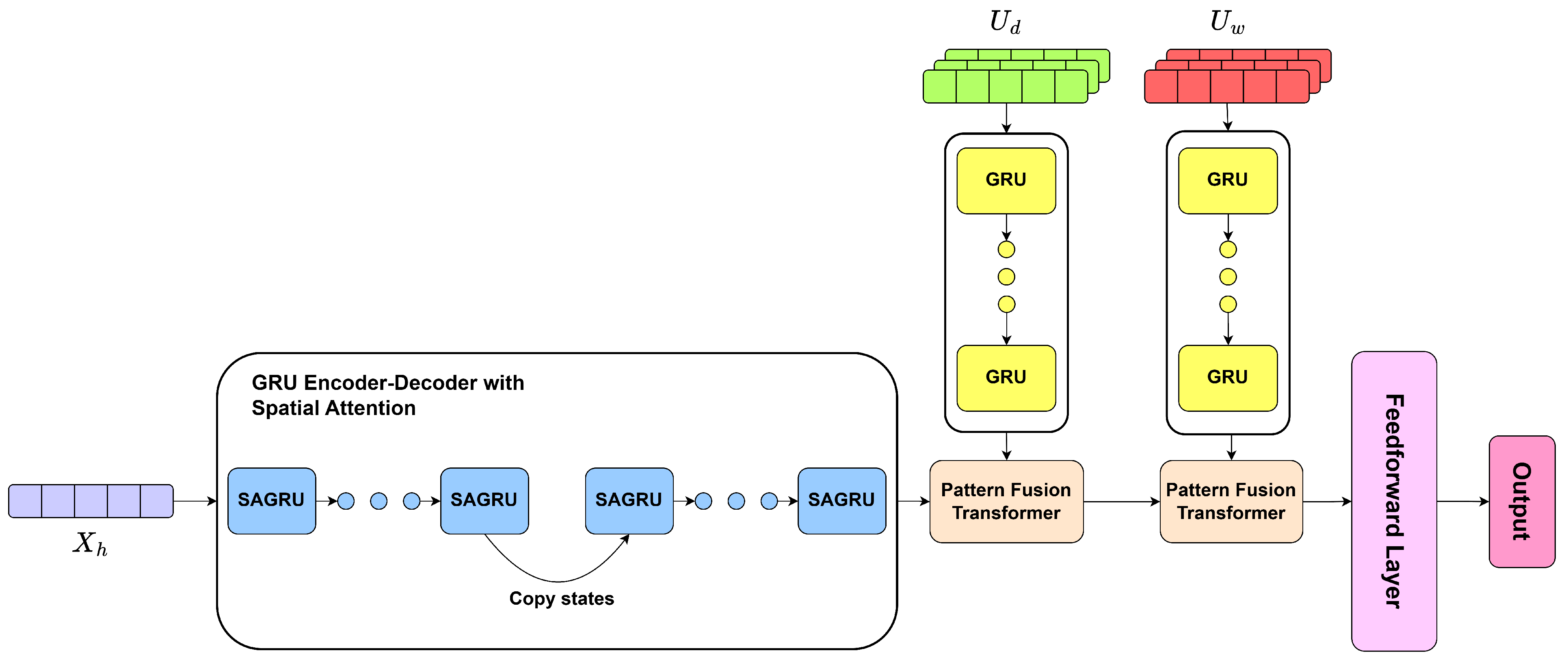
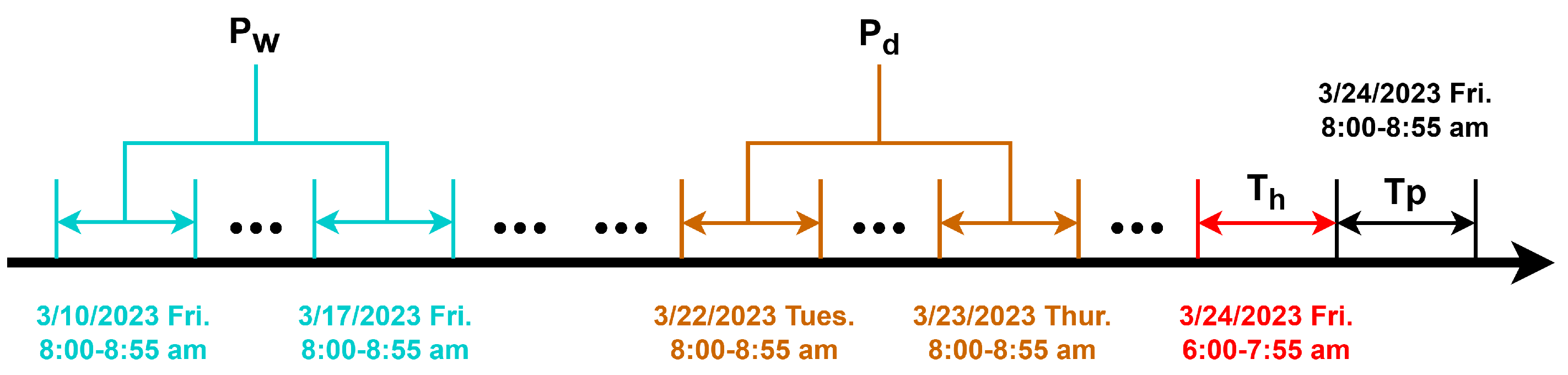
• We present a novel and interpretable perspective for handling periodicity traffic prediction data, aiming to use the different features of various types of periodicity data fully. Specifically, we utilize hourly data to forecast the basic future traffic pattern and introduce the Pattern Induction Block, which enables the induction of regular future traffic patterns from daily and weekly data. Furthermore, we propose the Pattern Fusion Transformer to consolidate these disparate outputs effectively.
• We propose the Spatial Attention GRU encoder–decoder to simultaneously consider spatial and temporal relationships. This spatial attention mechanism facilitates the dynamic computation of inter-node relationships at each time step. Consequently, it enhances the representation of the current traffic status while effectively capturing the evolving spatial correlations.
• We conduct extensive experimental evaluations to assess the model’s performance on four PEMS datasets. The resulting experimental findings reveal that GTPFN performs better than state-of-the-art baselines on most horizons.

The rest of this paper is organized as follows: An overview of the relevant work is provided in Section 2, the definition of the problem is provided in Section 3, the various parts of the model are discussed in detail in Section 4, and Section 5 provides our comparison with other baselines on PEMS datasets as well as sufficient ablation experiments, hyperparameter experiments, and their comparison results. Finally, we conclude in Section 6.

2. Related Work

2.1. Periodicity

In traffic prediction, recognizing and accommodating recurring traffic patterns, including daily rush hours, weekly fluctuations between weekdays and weekends, and seasonal variations, is paramount. These periodic features are instrumental for enhancing the performance of traffic prediction models. Consequently, researchers are dedicated to exploring methods for effectively capturing and utilizing this periodic information for traffic forecasting.

The Attention-Based Spatio-Temporal Graph Convolutional Network (ASTGCN) [16] puts periodic information into corresponding stacked spatio-temporal blocks composed of convolution and attention. It combines their outputs with a linear layer to obtain the final result. The Transformer-Graph Convolutional Attention Network (TRGCAT) [17] encodes periodic features based on temporal transformer layers in parallel and then concatenates and decodes them with the spatial feature through the Graph Convolutional Attention Network to obtain the final output. The Multi-View Dynamic Graph Convolution Network (MVDGCN) [18] puts periodic information into the GRU encoder–decoder with coupled graph convolution and fuses these results with linear layers. Multiple Information Spatio–Temporal Attention-Based Graph Convolution Networks (MISTAGCNs) [15] put the periodic information into the corresponding spatio-temporal blocks and then stack these results and put them into multiple spatio-temporal blocks to obtain the final result.

Nonetheless, many contemporary models incorporating periodicity, including the aforementioned ones, commonly integrate hourly, daily, and weekly data within a singular module to encompass spatio-temporal relationships, fusing them through straightforward mechanisms. These approaches neglect the characteristics inherent in distinct periodic information, thereby limiting the potential enhancement of the model’s performance. Specifically, the daily and weekly data that have the same prediction period are more conducive to induction. Daily data that are collected before the prediction period, on the other hand, are better suited for capturing the spatio-temporal relationships that are essential for predictive analytics. Furthermore, prevalent periodic data fusion techniques such as concatenation and linear layers, as employed in the aforementioned models, exhibit a degree of oversimplification in their capacity to comprehensively integrate and leverage periodic information.

2.2. Transformer

Transformer is a sequence-to-sequence model based on the self-attention mechanism [19], which is widely used in natural language processing methods, such as machine translation, text summarization, language generation, and other tasks [20,21]. It achieves significant results in a short period of time. Transformer adopts a new architecture compared to that used by the traditional Recurrent Neural Network (RNN) model. It does not need to process the elements in the sequence one-by-one, which makes the training process highly parallel and accelerates the training speed of the model. The self-attention mechanism is the core idea of Transformer. It can model the relationship between any two positions in a sequence, thereby capturing global contextual information. It also interacts with all other positions by computing an attention weight matrix. It subsequently combines and aggregates the representations of various positions, factoring in their respective attention weights. This method enables the model better to understand the dependency relationships between different sentence positions. In addition to the self-attention mechanism, Transformer introduces residual connections and layer normalization techniques to address gradient vanishing and stability issues during the training process.

Transformer has made significant achievements in traffic prediction due to its excellent ability to capture complex spatio-temporal relationships in historical data. Spatio-Temporal Transformer Networks (STTNs) [22] utilize the stacking of spatial transformers and temporal transformers to fuse spatio-temporal information. Autoformer [23] designs a decomposition architecture to deal with long-term temporal dependencies. It also creates an autocorrelation mechanism to improve the computation efficiency and data utilization. Non-Stationary Transformers [24] address the over-stationarization problem which deteriorates Transformer’s performance in non-stationary time series forecasting. It introduces two key modules,“Series Stationarization” to enhance the predictability by standardizing input statistics and “De-Stationary Attention” to restore non-stationary information into temporal dependencies. Propagation Delay-Aware Dynamic Long-Range Transformer (PDFormer) [25] introduces a spatial self-attention module incorporating distinct graph-masking techniques to capture local geographic and global semantic neighborhoods. Moreover, a traffic delay perception feature conversion module was devised to model temporal delays in the propagation of spatial information explicitly.

However, although various studies have demonstrated Transformer’s strong ability to capture spatio-temporal relationships, the vast memory consumption caused by excessive parameters must be addressed, especially when using the multi-head attention mechanism, which exacerbates this situation. Some models only stack Transformer blocks to achieve better prediction results while ignoring the vast memory consumption. Determining how to more efficiently utilize transformers to reduce memory usage while improving the model’s accuracy remains a challenging issue. Determining how to solve the problem mentioned above is also a key point that we are concerned about, so we use transformer blocks for pattern fusion instead of capturing spatio-temporal dependencies, which can significantly reduce the usage of transformers without harming the model’s performance.

3. Preliminaries

In this section, we provide the basic definitions and statements related to this work.

3.1. Road Network

The road map $G=(V,E,A)$ is used to display the connection relationship of road segments. $V={\left\{v_i\right\}}_{i=1,2,\cdots ,N}$ is a set of nodes on the road, and N represents the number of nodes. $E=\left\{e_{ij}\right\}$ is a set of edges indicating connectivity between node i and node j. $A\in R^{N\times N}$ describes the connectivity between nodes. The specific definition is as follows:

$$\begin{array}{c}{A}_{ij}=\left\{\begin{array}{cc}1,\hfill & \mathrm{if}{v}_i\mathrm{and}{v}_j\mathrm{are}\mathrm{connected},\hfill \\ 0,\hfill & \mathrm{otherwise}.\hfill \end{array}\right.\end{array}$$

(1)

While there is a definition of A in the standard traffic network diagram, this model uses dynamic matrices to capture changing spatial relationships, not fixed ones like A.

3.2. Traffic Feature Matrix

Assuming that a sequence of time T records the traffic features of each node in the road network G during this time period, we use $x_t^{c,i}\in R$ to indicate the value of the c-th feature of node i at time t. $X_t^i\in R^F$ denotes the values of all features of node i at time t, and F is the number of traffic features. $\mathbf{X}=(X_t^1,X_t^2,\dots ,X_t^N)\in R^{N\times F}$ shows the values of all nodes at time t. $\mathcal{X}=({\mathbf{X}}_1,{\mathbf{X}}_2,\dots ,{\mathbf{X}}_T)\in R^{N\times T\times F}$ denotes the value of all features of all nodes over the period T. In the experiment, we use the traffic flow for predictions for the PEMS03, 04, and 08 datasets, while for the PEMS-Bay dataset, we choose speed.

3.3. Problem Definition

To predict traffic information $Y=(y^1,y^2,\cdots ,y^N)\in R^{N\times T_p}$ for a while in the future, we utilize the $\mathcal{X}$ of specific periods in the past. Y represents the characteristics of all nodes in the next $T_p$ time steps. $y^i=(y_1^i,y_2^i,\dots ,y_{T_p}^i)\in R^{T_p}$ represents one traffic feature of a particular node i during the predicted period.

4. Methodology

4.1. Data Preparation and Processing

Before formally introducing the modules in our model, we need to introduce the data required for each module. As shown in Figure 1, ${\mathcal{X}}_h\in R^{N\times T_h\times F_i}$ denotes hourly data, and $T_h$ is the length of its time steps. $U_d=\left({\mathcal{X}}_d^1,\cdots ,{\mathcal{X}}_d^{P_d}\right)\in R^{P_d\times N\times T_p\times F_i}$ denotes daily data, namely those with the same time period as the predicted time in the previous $P_d$ days. Similarly, $U_w=\left({\mathcal{X}}_w^1,\cdots ,{\mathcal{X}}_w^{P_w}\right)\in R^{P_w\times N\times T_p\times F_i}$ denotes weekly data, namely those with the same time period as the predicted time in the previous $P_w$ weeks. For instance, as Figure 2 shows, if we want to predict the traffic feature from 8:00 to 8:55 on Friday, 24 March, we need data from 7:00 to 7:55 on 24 March (${\mathcal{X}}_h$), data from 8:00 to 9:00 on 23 March and 22 March ($U_d$), and data from 8:00 to 9:00 on 17 March and 10 March ($U_w$). The exact number of $P_d$ and $P_w$ to choose depends on the specific situation. It is important to emphasize that $F_i$ represents the input feature dimension, which has been modified from the original matrix containing only one traffic feature through a linear layer. This modification allows us to capture more complex relationships from the input features.

4.2. Overview

As shown in Figure 1, the GTPFN mainly consists of three modules. The first module is a Spatial Attention GRU encoder–decoder for hourly data. We integrate the GRU and spatial mechanism to capture the spatio-temporal relationship at each time step. The second module is the Pattern Induction Block for daily and weekly data. We utilize the GRU gate mechanism to induce the regular traffic pattern for the predicted period. The third module is the Pattern Fusion Transformer for periodic result fusion, We use the multi-head self-attention mechanism of Transformer to deeply fuse the periodic information results generated by the above two modules.

4.3. Spatial Attention GRU Encoder–Decoder

Firstly, we feed ${\mathcal{X}}_h\in R^{N\times T_h\times F_i}$ into a Spatial Attention GRU encoder–decoder to generate the candidate prediction outcome ${\tilde{Y}}_0$. Compared with the Long Short-Term Memory (LSTM) [26], the Gated Recurrent Unit (GRU) network has gained widespread adoption for its parameter efficiency and competitive ability to capture long-term temporal relationships [27], thereby serving as a preferred alternative to the LSTM. The basic formulas are as follows:

$$R_t=\sigma \left(I_t{W}_{xr}+H_{t-1}{W}_{hr}+b_r\right)$$

(2)

$$Z_t=\sigma \left(I_t{W}_{xz}+H_{t-1}{W}_{hz}+b_z\right)$$

(3)

$$\tilde{H}=tanh\left(I_t{W}_{xh}+\left(R_t\odot H_{t-1}\right)W_{hh}+b_h\right)$$

(4)

$$H_t=Z_t\odot H_{t-1}+(1-Z_t)\odot \widetilde{H_t}$$

(5)

where $R_t$ and $Z_t$ represent the reset gate and the update gate, respectively, which are the core of the GRU. $I_t$ is the input at the current time t. $H_{t-1}$ shows the hidden state of the previous time step. $\tilde{H}$ indicates the candidate hidden state. $H_t$ is the final hidden state of time step t. ⊙ represents the Hadamard product. $R_t$ is used to control the impact of historical information on the current hidden state at a time point. When it is 0, it means completely ignoring historical information; when it is 1, it means retaining more historical information. The update gate $Z_t$ is used to determine the weights of the hidden state of the previous time step and the candidate hidden state of the current time step. When it approaches 1, it means that the hidden state of the previous time step has a greater impact on the current time than the current input data.

In order to effectively model the dynamic spatial dependencies over time while considering the temporal dependencies, we replace the above formulas with the following:

$$S=Leaky\_ReLU\left({\mathbf{X}}_{\mathbf{t}}^{\mathbf{h}}{W}_{xa}{\left(H_{t-1}{W}_{ha}\right)}^T\right)$$

(6)

$$S_{i,j}^{\prime }=\frac{exp\left(S_{i,j}\right)}{{\sum }_{j=1}^{N}exp\left(S_{i,j}\right)}$$

(7)

$${\mathbf{X}}_{\mathbf{t}}^{{\mathbf{h}}^{\prime }}=S^{\prime }{\mathbf{X}}_{\mathbf{t}}^{\mathbf{h}}{R}_t=\sigma \left({\mathbf{X}}_{\mathbf{t}}^{{\mathbf{h}}^{\prime }}{W}_{xr}+b_r\right)$$

(8)

$$Z_t=\sigma \left({\mathbf{X}}_{\mathbf{t}}^{{\mathbf{h}}^{\prime }}{W}_{xz}+b_z\right)$$

(9)

$$\tilde{H}=tanh\left({\mathbf{X}}_{\mathbf{t}}^{\mathbf{h}}{W}_{xh}+\left(R_t\odot H_{t-1}\right)W_{hh}+b_h\right)$$

(10)

$$H_t=Z_t\odot H_{t-1}+(1-Z_t)\odot \widetilde{H_t}$$

(11)

where ${\mathbf{X}}_{\mathbf{t}}^{\mathbf{h}}\in R^{N\times F_i}$ is the hourly input of the current step. $S\in R^{N\times N}$ is the attention score between nodes at time t, and $S^{\prime }\in R^{N\times N}$ is the result of normalization through the Softmax function. ${\mathbf{X}}_{\mathbf{t}}^{{\mathbf{h}}^{\prime }}$ is the result after spatial attention. $\tilde{H},H_{t-1},H_t\in R^{N\times F_h}$ denote the candidate hidden state, the hidden state of the previous time step, and the hidden state of the current time step, respectively. $W_{xa},W_{xr},W_{xz},W_{xh}\in R^{F_i\times F_h}$, $W_{hr},W_{hz},W_{hh}\in R^{F_h\times F_h}$ and $b\in R^{N\times F_h}$ are learnable parameters. $F_h$ is the feature dimension of the hidden state.

As shown in Equations (6)–(11), we first calculate the attention score according to ${\mathbf{X}}_{\mathbf{t}}^{\mathbf{h}}$ and $H_{t-1}$ and then capture spatial relationships to obtain ${\mathbf{X}}_{\mathbf{t}}^{{\mathbf{h}}^{\prime }}$ through spatial attention. This departure enables the independent utilization of spatial information obtained from each time step. As a result, our model is able to incorporate spatial attention into the GRU computations, thus enhancing its capacity to capture dynamic spatial correlations effectively.

We use this Spatial Attention GRU encoder to obtain the hidden state of the historical time series, which contains essential historical contextual information. Then, we use the Spatial Attention GRU decoder to generate candidate prediction autoregressive results ${\tilde{Y}}_0\in R^{T_p\times N\times F_h}$ based on this hidden state.

4.4. Pattern Induction Block

The Spatial Attention GRU encoder–decoder model employs hourly data as the foundation for prediction, while the Pattern Induction Block harnesses daily and weekly historical information to abstract the conventional traffic pattern during the predicted timeframe. The Pattern Induction Block is composed of GRU layers. The number of layers is $P_d$ for daily data and $P_w$ for weekly data. The formulas of GRU layers are very similar to Equations (2)–(5). We only replace $I_t$ with ${\mathcal{X}}_t\in R^{N\times T_p\times F_i}$. The utilization of the GRU layer serves the purpose of leveraging its gate mechanism to eliminate outliers within the periodic information effectively. This transformative approach aims to attain the regular traffic pattern during the predicted period rather than exploiting the GRU layer to address spatio-temporal relationships as usual. Taking the daily part as an example, we introduce the specific working method of the Pattern Induction Block in detail below.

Daily data are $U_d\in R^{P_d\times N\times T_p\times F_i}$, and their GRU layers of the Pattern Induction Block should be $P_d$, corresponding to the past $P_d$ days. Each ${\mathcal{X}}_d^i\left(i=1,2,\cdots ,P_d\right)$ in $U_d$ is put into the GRU layers from old to new, and finally, we obtain the daily traffic pattern $H_d\in R^{N\times T_p\times F_h}$. Similarly, the weekly regular pattern $H_w\in R^{N\times T_p\times F_h}$ is also obtained using the same method.

4.5. Pattern Fusion Transformer

After obtaining the candidate prediction result ${\tilde{Y}}_0$, daily traffic pattern $H_d$, and weekly traffic pattern $H_w$ based on the periodic information, we fuse them sequentially in the Pattern Fusion Transformer. The Transformer mainly consists of position encoding, a multi-head self-attention mechanism, the Feedforward layer, and the residual connection & normalization layer, as shown in Figure 3.

In contrast to Recurrent Neural Networks (RNNs), which inherently exhibit a natural temporal sequencing of data and iterate input following this temporal order, the Transformer architecture’s self-attention mechanism lacks an intrinsic awareness of input sequences’ temporal relationships. The time order is important for the fusion of regular traffic patterns and candidate prediction results, because they should pay more attention to the information of nearby time points rather than the information of distant time points. Consequently, it becomes imperative to introduce position encoding as a remedy for this limitation. Position encoding leverages sine (sin) and cosine (cos) functions to encode and represent the temporal relationships among input samples. The computational procedure for position encoding is elucidated by Formulas (12) and (13).

$$P{E}_{(pos,2i)}=sin\left(\frac{pos}{{10,000}^{2i/d_{model}}}\right)$$

(12)

$$P{E}_{(pos,2i+1)}=cos\left(\frac{pos}{{10,000}^{2i/d_{model}}}\right)$$

(13)

In this context, $pos$ denotes the specific position of the current sample within the input sequence, $d_{model}$ signifies the eigenvalue dimensions of each sample, and i denotes the position of the current feature within the sample. The position encoding matrix, represented as $PE$, is constructed by iteratively encoding information concerning the sample’s position and feature positions. This encoding process uses the sine (sin) and cosine (cos) functions. This matrix has a dimensionality of $pos\ast d_{model}$. The rationale behind employing sine and cosine functions is their ability to capture relative position relationships effectively. Specifically, any location $P{E}_{pos+k}$ within the encoding matrix can be expressed as a linear function of $P{E}_{pos}$, as shown in Equations (14) and (15). This property simplifies the extraction of relative positional information between the two positions.

$$sin(pos+k)=sin\left(pos\right)cosk+cos\left(pos\right)sink$$

(14)

$$cos(pos+k)=cos\left(pos\right)cosk-sin\left(pos\right)sink$$

(15)

Finally, the outcome of the positional encoder is added to the input, so that the temporal relationship is preserved for further calculation.

After applying positional encoding, we utilize the self-attention mechanism to uncover the deep-seated interconnections within periodic data. Our goal is to enable our model to adeptly capture and encapsulate the inherent periodic correlations in time series data, thereby enhancing the understanding of the relationships between the candidate prediction outcome and regular traffic patterns. Applying this method, in turn, facilitates the generation of more comprehensive representations and precise analytical insights for traffic prediction. The formulas used for the self-attention of the block are as follows (here, we collectively refer to $H_d$ and $H_w$ as O):

$$Q={\tilde{Y}}_{i-1}{W}_q$$

(16)

$$K=H{W}_k$$

(17)

$$V=H{W}_v$$

(18)

$$SelfAttention(Q,K,V)=softmax\left(\frac{Q{\left(K\right)}^T}{\sqrt{F_k}}\right)V$$

(19)

where Q, K, and V represent the query, key, and value, respectively. $W_q\in R^{F_h\times F_k},W_k\in R^{F_h\times F_k},W_v\in R^{F_h\times F_k}$ are learnable parameters. $F_k$ is the dimension of the key that is used to adjust the similarity calculation range between queries and keys. $softmax$ is employed to calculate its correlation coefficient, ensuring that its product values adhere strictly to the positivity and collectively sum up to 1. Subsequently, the value matrix V undergoes a weighted aggregation procedure using predetermined weight coefficients, leading to the attainment of the self-attention output.

This module aims to integrate periodic traffic patterns into the candidate prediction results. Therefore, for the calculation of Q and V, we choose to use the periodic traffic pattern H, and for the calculation of K, we choose to use ${\tilde{Y}}_{i-1}$. In order to capture the correlation and dependency between patterns and the candidate prediction results at a deeper level, we also use the multi-head attention mechanism for the calculation, and the specific formula is as follows:

$$MultiHead(Q,K,V)=\mathrm{Concat}(h_1,\cdots ,h_n)$$

(20)

$$h_j=SelfAttention(H{W}_j^Q,{\tilde{Y}}_{i-1}{W}_i^K,H{W}_j^V)$$

(21)

The multi-head self-attention mechanism is an amalgamation of multiple self-attention operations that employs several self-attention heads to capture distinct subspaces of information. The resulting attention values from each head are then concatenated and subjected to linear transformation, yielding the ultimate attention representation. Taking the n-head self-attention mechanism as an example, the input feature vector X is partitioned into $X//n$ sub-feature sequences, where $//$ means the division with only the retention of the integer part. Each sub-sequence independently computes its attention and subsequently merges them into an output sequence denoted as O through concatenation.

It should be emphasized that, after obtaining the output sequence $O\in R^{N\times T_p\times F_h}$, we add the periodic fusion information ${\tilde{Y}}_{i-1}$ from the previous step in the form of residuals and then perform LayerNorm together to improve the stability of the gradient propagation and enhance the feature representation ability. The final output result ${\tilde{Y}}_i$ of this Pattern Fusion Transformer is obtained through LayerNorm and a Feedforward layer. The formula can be expressed as follows:

$$L_i=LayerNorm(O+{\tilde{Y}}_{i-1})$$

(22)

$${\tilde{Y}}_i=ReLU(ReLU(L_i{W}_{ia}+b_{ia})W_{ib}+b_{ib})$$

(23)

where $W_{ia}\in R^{F_h\times 2F_h}$, $W_{ib}\in R^{2F_h\times F_h}$ are learnable parameters.

In this way, we only used two Transformer blocks to deeply capture the internal connections between periodic information and combine them, reducing memory usage while still giving the model excellent predictive power.

After passing through the Weekly Pattern Fusion Transformer, the output obtained is ${\tilde{Y}}_2$. It passes through a Feedforward layer to adjust the feature dimension and perform feature extraction, resulting in the final model output result Y. The specific formula for this last Feedforward network is as follows:

$$Y=ReLU({\tilde{Y}}_2{W}_{ya}+b_{ya})W_{yb}+b_{yb}$$

(24)

5. Experiment

5.1. Datasets

Our experiments use four Caltrans Performance Measurement System datasets to evaluate our model: PEMS-Bay, PEMS04, PEMS07, and PEMS08 [28]. PEMS provides a unified database of traffic data collected by Caltrans on California’s highways, along with datasets from Caltrans and partner agencies. The PEMS04, 07, and 08 datasets contain three traffic features, flow, speed, and occupation, while the PEMS-Bay dataset only contains the speed feature. The relevant information from these datasets is shown in

Table 1. Dataset description and statistics.

Dataset	#Sensors	Granularity	#Time Step	Time Range
PEMS-Bay	325	5 min	52,116	01/01/2017–06/31/2017
PEMS04	307	5 min	16,992	01/01/2018–02/28/2018
PEMS07	883	5 min	28,224	05/01/2017–08/31/2017
PEMS08	170	5 min	17,856	07/01/2016–08/31/2016

.

5.2. Baselines

In order to substantiate the efficacy of our proposed method, we compare our method with the following baseline methods:

• HA: A statistical method that employs historical data averages to forecast forthcoming values.
• ARIMA [29]: A methodology that integrates autoregressive and moving average models to address time series forecasting challenges.
• VAR [30]: A statistical method used for modeling and analyzing the dynamic relationships among multiple time series variables.
• FC-LSTM [31]: A neural network architecture that combines fully connected layers with Long Short-Term Memory (LSTM) layers to handle sequential and non-sequential data.
• DCRNN [32]: A model that combines the bi-directional random walk on the distance-based graph with GRU in an encoder–decoder manner.
• Graph WaveNet [33]: A framework that combines the adaptive adjacency matrix into graph convolution with 1D dilated convolution.
• ASTGCN [16]: A model which utilizes attention and convolution to capture the spatio-temporal relationship with periodicity fusion.
• STGCN [13]: A method that utilizes graph convolution and casual convolution to learn the spatial and temporal dependencies.
• STSGCN [34]: A network that utilizes the localized spatio-temporal subgraph module to model localized correlations independently.
• STID [35]: A framework that leverages Spatial and Temporal IDentity information (STID) to address samples’ indistinguishability in the spatial and temporal dimensions based on multi-layer perceptrons.

5.3. Evaluation Metrics

To facilitate a quantitative comparison of these methodologies, we employ three distinct metrics to comprehensively evaluate the model’s performance in traffic forecasting. Specifically, these metrics encompass the Mean Absolute Error (MAE), Root Mean Square Error (RMSE), and Mean Absolute Percentage Error (MAPE), each of which is elucidated as follows:

$$MAE=\frac{1}{NT}\sum _{i=1}^N\sum _{t=1}^T\left|{\widehat{y}}_t^i-y_t^i\right|$$

(25)

$$MAPE=\frac{100\%}{NT}\sum _{i=1}^N\sum _{t=1}^T\left|\frac{{\widehat{y}}_t^i-y_t^i}{y_t^i}\right|$$

(26)

$$RMSE=\sqrt{\frac{1}{NT}{\displaystyle \sum _{i=1}^N}{\displaystyle \sum _{t=1}^T}{\left({\widehat{y}}_t^i-y_t^i\right)}^2}$$

(27)

where ${\widehat{y}}_t^i$ is the element in the predicted result $\widehat{\mathit{Y}}$, and $y_t^i$ is the element in the ground truth $\mathit{Y}$.

5.4. Experiment Setting

All experimental assessments are conducted utilizing a single NVIDIA RTX 3090 GPU with 24 GB of memory. The proposed neural network architecture is implemented by utilizing PyTorch. The maximum training epoch is established at 300, including an early stopping mechanism. The default batch size is 64. The key hyperparameters are configured as follows: $T_h$ is 12, equivalent to the past 1 h; $P_d$ and $P_w$ are both 2, corresponding to the past 2 days and 2 weeks, respectively. There are 32 hidden channels for the GRU layers, and the number of heads of multi-head attention is eight. The initial learning rate for the model is initialized at 0.01 and subsequently reduced to 0.001 after 150 training epochs. The weight decay is 0.0001. Regarding dataset partitioning, the training, validation, and test data are distributed in a ratio of 6:2:2. Model training is executed by employing the Adam optimization algorithm, and the loss function is the SmoothL1 Loss. We utilize the above-mentioned hourly, daily, and weekly data to forecast the subsequent 12 time steps (i.e., one hour).

5.5. Main Results

Table 2. Traffic Forecasting Result Comparison On Different Datasets.

Datasets	Methods	Horizon 3			Horizon 6			Horizon 12
		MAE	RMSE	MAPE	MAE	RMSE	MAPE	MAE	RMSE	MAPE
PEMS-Bay	HA	2.88	5.59	6.77%	2.88	5.59	6.77%	2.88	5.59	6.77%
	ARIMA	1.62	3.30	3.50%	2.33	4.76	5.40%	3.38	6.50	8.30%
	VAR	1.74	3.16	3.60%	2.32	4.25	5.00%	2.93	5.44	6.50%
	FC-LSTM	2.05	4.19	4.80%	2.20	4.55	5.20%	2.37	4.96	5.70%
	DCRNN	1.39	2.80	2.73%	1.66	3.81	3.75%	1.98	4.64	4.75%
	Graph WaveNet	1.39	2.80	2.69%	1.65	3.75	3.65%	1.97	4.58	4.63%
	ASTGCN	1.52	3.13	3.22%	2.01	4.27	4.48%	2.61	5.42	6.00%
	STGCN	1.35	2.86	2.86%	1.69	3.83	3.85%	2.00	4.56	4.74%
	STSGCN	1.44	3.01	3.04%	1.83	4.18	4.17%	2.26	5.21	5.40%
	STID	1.30	2.81	2.73%	1.62	3.72	3.68%	1.89	4.40	4.47%
	GTPFN	1.31	2.75	2.65%	1.62	3.65	3.52%	1.90	4.35	4.29%
PEMS04	HA	30.26	60.93	72.24%	30.26	60.93	72.24%	30.26	60.93	72.24%
	ARIMA	21.98	35.21	16.52%	25.38	39.21	21.03%	26.67	40.74	22.43%
	VAR	21.94	34.40	16.42%	23.72	36.58	18.02%	26.76	40.28	20.94%
	FC-LSTM	21.37	33.31	15.21%	23.72	36.58	18.02%	26.76	40.28	20.94%
	DCRNN	19.65	31.29	15.17%	21.80	34.11	16.83%	26.20	39.91	18.43%
	Graph WaveNet	18.75	29.80	14.14%	20.40	31.91	15.85%	23.21	35.41	19.43%
	STGCN	19.70	31.15	14.83%	20.70	32.86	15.28%	22.14	34.99	16.92%
	ASTGCN	20.16	31.53	14.13%	22.29	34.27	15.65%	26.23	40.12	19.19%
	STSGCN	19.80	31.58	13.41%	21.30	33.84	14.27%	24.47	38.84	16.27%
	STID	17.52	28.48	12.00%	18.29	29.86	12.46%	19.58	31.79	13.38%
	GTPFN	17.72	29.74	11.82%	18.51	31.24	12.18%	19.87	33.42	13.00%
PEMS07	HA	37.59	51.65	21.83%	37.59	51.65	21.83%	37.59	51.65	21.83%
	ARIMA	32.02	48.83	18.30%	35.18	52.91	20.54%	38.12	55.64	20.77%
	VAR	20.09	32.13	13.61%	25.58	40.41	17.44%	32.86	52.05	26.00%
	FC-LSTM	20.42	33.21	8.79%	23.18	37.54	9.80%	28.73	45.63	12.23%
	DCRNN	19.45	31.39	8.29%	21.18	34.42	9.01%	24.14	38.84	10.42%
	Graph WaveNet	18.69	30.69	8.02%	20.26	33.37	8.56%	22.79	37.11	9.73%
	STGCN	20.33	32.73	8.68%	21.66	35.35	9.16%	22.74	37.94	9.71%
	ASTGCN	21.36	32.91	8.87%	22.63	36.45	9.86%	24.51	37.97	11.03%
	STSGCN	20.21	31.65	8.46%	21.45	33.95	8.96%	23.99	39.36	10.13%
	STID	18.31	30.39	7.72%	19.59	32.90	8.30%	21.52	36.29	9.15%
	GTPFN	17.32	29.88	7.16%	18.38	31.96	7.56%	20.00	34.74	8.32%
PEMS08	HA	29.52	44.03	16.59%	29.52	44.03	16.59%	29.52	44.03	16.59%
	ARIMA	19.56	29.78	12.45%	22.35	33.43	14.43%	26.27	38.86	17.38%
	VAR	19.52	29.73	12.54%	22.25	33.30	14.23%	26.17	38.97	17.32%
	FC-LSTM	17.38	26.27	12.63%	21.22	31.97	17.32%	30.96	43.96	25.72%
	DCRNN	16.62	25.48	10.04%	17.88	17.63	11.38%	22.51	34.21	14.17%
	Graph WaveNet	14.22	22.96	9.45%	15.94	24.72	9.77%	17.27	26.77	11.26%
	STGCN	15.45	25.13	9.98%	17.79	27.38	11.03%	21.46	33.71	13.34%
	ASTGCN	16.45	25.18	11.13%	18.76	28.57	12.33%	22.53	33.69	15.34%
	STSGCN	16.65	25.40	10.90%	17.82	27.31	11.60%	19.77	31.43	13.12%
	STID	13.28	21.66	8.62%	14.21	23.57	9.24%	15.58	25.89	10.33%
	GTPFN	12.95	21.93	8.94%	13.57	23.28	9.41%	14.47	25.40	10.34%

shows a comparison of the baselines for 15 min (horizon = 3), 30 min (horizon = 6), and 60 min (horizon = 12) ahead of the prediction on the PEMS datasets. We observe that (1) deep learning techniques, exemplified by STSGCN and DCRNN, consistently yield superior outcomes when compared to conventional time series methodologies, such as the ARIMA and VAR models. This result substantiates the efficacy of incorporating both spatial and temporal correlations in traffic forecasting. (2) STID achieves promising results on all four datasets, indicating the importance of considering spatio-temporal indistinguishability in the sample. (3) The GTPFN model yields commendable outcomes compared to preceding state-of-the-art models across four distinct datasets. This performance underscores the methodology’s effectiveness, which incorporates periodic information for predictive and inductive purposes alongside the seamless integration of Pattern Fusion Transformers. Such an approach is demonstrably efficacious for bolstering the precision of both short-term and long-term forecasting endeavors.

5.6. Ablation Study

We conducted ablation studies on the PEMS04 dataset to validate the effectiveness of the key components of our proposed model GTPFN. We name the GTPFNs without different components as follows:

• GTPFN w/o P: Removes the utilization of daily data and weekly data and only uses hourly data for predictions.
• GTPFN w/o T: Removes the Pattern Fusion Transformer and fuses the periodical data by linear layers instead.
• GTPFN w/o H: Removes the utilization of hourly data and only uses daily data and weekly data to induce the pattern.
• GTPFN w/o A: Removes the attention mechanism from the SAGRU encoder–decoder.

Figure 4 shows the results of the ablation experiment. Evidently, the Pattern Induction Block exerts the most substantial influence on the entire model, particularly in the context of long-term predictions. This observation underscores the pivotal role that Pattern Induction Blocks play in mitigating the cumulative error impact of the GRU encoder–decoder. The second-most influential factor affecting the model’s performance is the Pattern Fusion Transformer, underscoring the imperative of delving into deeper levels to consider the interplay of periodic information. Importantly, it is noteworthy that when employing only the Pattern Induction Block for prediction, the loss values exhibit remarkable uniformity across various time points. This outcome aligns coherently with our expectations, as utilizing the induced regular traffic patterns as predictive outcomes does not entail the stepwise accumulation of losses that is characteristic of conventional prediction models.

5.7. Hyperparameter Experiments

In this subsection, we conduct hyperparameter experiments using the PEMS04 dataset to determine the optimal values for $P_d$ and $P_w$. The outcomes are visually represented in Figure 5. The most favorable prediction results are obtained when the values of $P_d$ and $P_w$ are both 2. This observation underscores the significance of amalgamating weekly and daily information to enhance the prediction accuracy. Notably, the model’s performance is the least favorable when $P_d$ is 2 and $P_w$ is 0, while it is significantly improved when $P_d$ is 0 and $P_w$ is 2. This discrepancy implies that the weekly periodicity within the PEMS04 dataset holds greater prominence compared to the daily periodicity.

6. Conclusions

This paper proposes a novel GRU- and Transformer-Based Periodicity Fusion Network (GTPFN). The proposed model includes the Spatial Attention GRU encoder–decoder. It captures dynamic spatio-temporal relationships at each time step and makes basic predictions based on hourly data. Additionally, the model incorporates Pattern Induction Blocks based on GRU layers. This block induces regular traffic patterns using daily and weekly data. Furthermore, the model utilizes Pattern Fusion Transformers to integrate the output from the above-mentioned modules, followed by a Feedforward layer to generate the final output. The extensive experiments on PEMS datasets demonstrate the superiority of the proposed method.

Nevertheless, this model exhibits a limited responsiveness towards the outlier. In future investigations, we intend to explore methodologies to integrate external influences from weather conditions, events, and accidents into the model, thereby fostering enhanced sensitivity towards the outlier. However, integrating these external influences poses potential challenges that warrant careful consideration. Challenges may include data quality issues, the dynamic nature of external factors, and the need for real-time updates. Addressing these challenges is crucial for ensuring the robustness of our predictive model. If the model can successfully address these challenges, it will be more sensitive to traffic flow prediction in emergencies, thereby achieving a better performance.

References

1. Guo, K.; Wu, Z.; Wang, W.; Ren, S.; Zhou, X.; Gadekallu, T.R.; Luo, E.; Liu, C. GRTR: Gradient Rebalanced Traffic Sign Recognition for Autonomous Vehicles. IEEE Trans. Autom. Sci. Eng. 2023, 1–13. [Google Scholar] [CrossRef]
2. Yang, Y.; Wang, W.; Liu, L.; Dev, K.; Qureshi, N.M.F. AoI Optimization in the UAV-Aided Traffic Monitoring Network Under Attack: A Stackelberg Game Viewpoint. IEEE Trans. Intell. Transp. Syst. 2023, 24, 932–941. [Google Scholar] [CrossRef]
3. Zhang, G.P. Time series forecasting using a hybrid ARIMA and neural network model. Neurocomputing 2003, 50, 159–175. [Google Scholar] [CrossRef]
4. Zhang, L.; Liu, Q.C.; Yang, W.; Wei, N.; Dong, D. An Improved K-nearest Neighbor Model for Short-term Traffic Flow Prediction. Procedia Soc. Behav. Sci. 2013, 96, 653–662. [Google Scholar] [CrossRef]
5. Zivot, E.; Wang, J. Vector Autoregressive Models for Multivariate Time Series. In Modeling Financial Time Series with S-Plus®; Springer: New York, NY, USA, 2003; pp. 369–413. [Google Scholar] [CrossRef]
6. Ma, X.; Dai, Z.; He, Z.; Na, J.; Wang, Y.; Wang, Y. Learning Traffic as Images: A Deep Convolutional Neural Network for Large-Scale Transportation Network Speed Prediction. Sensors 2017, 17, 818. [Google Scholar] [CrossRef] [PubMed]
7. Yao, H.; Wu, F.; ke, J.; Tang, X.; Jia, Y.; Lu, S.; Gong, P.; Ye, J. Deep Multi-View Spatial-Temporal Network for Taxi Demand Prediction. In Proceedings of the AAAI Conference on Artificial Intelligence, New Orleans, LA, USA, 2–7 February 2018; Volume 32. [Google Scholar] [CrossRef]
8. Zhang, J.; Zheng, Y.; Qi, D. Deep Spatio-Temporal Residual Networks for Citywide Crowd Flows Prediction. In Proceedings of the AAAI Conference on Artificial Intelligence, Phoenix, AZ, USA, 12–17 February 2016; Volume 31. [Google Scholar] [CrossRef]
9. Ubal Núñez, C.; Di-Giorgi, G.; Contreras-Reyes, J.; Salas, R. Predicting the Long-Term Dependencies in Time Series Using Recurrent Artificial Neural Networks. Mach. Learn. Knowl. Extr. 2023, 5, 1340–1358. [Google Scholar] [CrossRef]
10. Zhao, L.; Song, Y.; Zhang, C.; Liu, Y.; Wang, P.; Lin, T.; Deng, M.; Li, H. T-GCN: A Temporal Graph Convolutional Network for Traffic Prediction. IEEE Trans. Intell. Transp. Syst. 2020, 21, 3848–3858. [Google Scholar] [CrossRef]
11. Ye, J.; Sun, L.; Du, B.; Fu, Y.; Xiong, H. Coupled Layer-wise Graph Convolution for Transportation Demand Prediction. In Proceedings of the AAAI Conference on Artificial Intelligence, Virtual, 2–7 February 2021; Volume 35, pp. 4617–4625. [Google Scholar] [CrossRef]
12. Xu, Y.; Cai, X.; Wang, E.; Liu, W.; Yang, Y.; Yang, F. Dynamic traffic correlations based spatio-temporal graph convolutional network for urban traffic prediction. Inf. Sci. 2022, 621, 580–595. [Google Scholar] [CrossRef]
13. Yu, B.; Yin, H.; Zhu, Z. Spatio-Temporal Graph Convolutional Networks: A Deep Learning Framework for Traffic Forecasting. In Proceedings of the Twenty-Seventh International Joint Conference on Artificial Intelligence, IJCAI-18, Stockholm, Sweden, 13–19 July 2018; AAAI Press Inc.: Menlo Park, CA, USA, 2018; pp. 3634–3640. [Google Scholar] [CrossRef]
14. Zhang, W.; Zhang, C.; Tsung, F. Transformer Based Spatial-Temporal Fusion Network for Metro Passenger Flow Forecasting. In Proceedings of the 2021 IEEE 17th International Conference on Automation Science and Engineering (CASE), Lyon, France, 23–17 August 2021; pp. 1515–1520. [Google Scholar]
15. Tao, S.; Zhang, H.; Yang, F.; Wu, Y.; Li, C. Multiple Information Spatial-Temporal Attention based Graph Convolution Network for traffic prediction. Appl. Soft Comput. 2023, 136, 110052. [Google Scholar] [CrossRef]
16. Guo, S.; Lin, Y.; Feng, N.; Song, C.; Wan, H. Attention Based Spatial-Temporal Graph Convolutional Networks for Traffic Flow Forecasting. In Proceedings of the AAAI Conference on Artificial Intelligence, Honolulu, HI, USA, 27 January–1 February 2019; Volume 33, pp. 922–929. [Google Scholar] [CrossRef]
17. Zhu, C.; Yu, C.X.; Huo, J. Research on Spatio-Temporal Network Prediction Model of Parallel-Series Traffic Flow Based on Transformer and Gcat. SSRN Electron. J. 2022. [Google Scholar] [CrossRef]
18. Huang, X.; Ye, Y.; Yang, X.; Xiong, L. Multi-view dynamic graph convolution neural network for traffic flow prediction. Expert Syst. Appl. 2023, 222, 119779. [Google Scholar] [CrossRef]
19. Vaswani, A.; Shazeer, N.; Parmar, N.; Uszkoreit, J.; Jones, L.; Gomez, A.N.; Kaiser, L.; Polosukhin, I. Attention is All You Need. In Proceedings of the NIPS’17: 31st International Conference on Neural Information Processing Systems, Long Beach, CA, USA, 4–9 December 2017; Curran Associates Inc.: Red Hook, NY, USA, 2017; pp. 6000–6010. [Google Scholar]
20. Liu, Z.; Lin, Y.; Cao, Y.; Hu, H.; Wei, Y.; Zhang, Z.; Lin, S.; Guo, B. Swin Transformer: Hierarchical Vision Transformer using Shifted Windows. In Proceedings of the 2021 IEEE/CVF International Conference on Computer Vision (ICCV), Montreal, QC, Canada, 10–17 October 2021; pp. 9992–10002. [Google Scholar]
21. Dai, Z.; Yang, Z.; Yang, Y.; Carbonell, J.G.; Le, Q.V.; Salakhutdinov, R. Transformer-XL: Attentive Language Models beyond a Fixed-Length Context. arXiv 2019, arXiv:1901.02860. [Google Scholar]
22. Xu, M.; Dai, W.; Liu, C.; Gao, X.; Lin, W.; Qi, G.J.; Xiong, H. Spatial-Temporal Transformer Networks for Traffic Flow Forecasting. arXiv 2020, arXiv:2001.02908. [Google Scholar]
23. Wu, H.; Xu, J.; Wang, J.; Long, M. Autoformer: Decomposition Transformers with Auto-Correlation for Long-Term Series Forecasting. arXiv 2022, arXiv:2106.13008. [Google Scholar]
24. Liu, Y.; Wu, H.; Wang, J.; Long, M. Non-stationary Transformers: Exploring the Stationarity in Time Series Forecasting. arXiv 2022, arXiv:2205.14415. [Google Scholar]
25. Jiang, J.; Han, C.; Zhao, W.X.; Wang, J. PDFormer: Propagation Delay-Aware Dynamic Long-Range Transformer for Traffic Flow Prediction. arXiv 2023, arXiv:2301.07945. [Google Scholar] [CrossRef]
26. Hochreiter, S.; Schmidhuber, J. Long Short-Term Memory. Neural Comput. 1997, 9, 1735–1780. [Google Scholar] [CrossRef] [PubMed]
27. Chung, J.; Gülçehre, Ç.; Cho, K.; Bengio, Y. Empirical Evaluation of Gated Recurrent Neural Networks on Sequence Modeling. arXiv 2014, arXiv:1412.3555. [Google Scholar]
28. Chen, C.; Varaiya, P.P. Freeway Performance Measurement System (Pems); PATH Research Report; Sage: Thousand Oaks, CA, USA, 2002. [Google Scholar]
29. Box, G.E.P.; Jenkins, G. Time Series Analysis, Forecasting and Control; Holden-Day, Inc.: Oakland, CA, USA, 1990. [Google Scholar]
30. Brockwell, P.J.; Davis, R.A. Time Series: Theory and Methods; Springer Science & Business Media: Berlin/Heidelberg, Germany, 2013. [Google Scholar]
31. Sutskever, I.; Vinyals, O.; Le, Q.V. Sequence to Sequence Learning with Neural Networks. arXiv 2014, arXiv:1409.3215. [Google Scholar]
32. Li, Y.; Yu, R.; Shahabi, C.; Liu, Y. Diffusion Convolutional Recurrent Neural Network: Data-Driven Traffic Forecasting. arXiv 2017, arXiv:1707.01926. [Google Scholar]
33. Wu, Z.; Pan, S.; Long, G.; Jiang, J.; Zhang, C. Graph WaveNet for Deep Spatial-Temporal Graph Modeling. In Proceedings of the Twenty-Eighth International Joint Conference on Artificial Intelligence, IJCAI-19, Macao, China, 10–16 August 2019; AAAI Press Inc.: Menlo Park, CA, USA, 2019; pp. 1907–1913. [Google Scholar] [CrossRef]
34. Song, C.; Lin, Y.; Guo, S.; Wan, H. Spatial-Temporal Synchronous Graph Convolutional Networks: A New Framework for Spatial-Temporal Network Data Forecasting. In Proceedings of the AAAI Conference on Artificial Intelligence, New York, NY, USA, 7–12 February 2020; Volume 34, pp. 914–921. [Google Scholar] [CrossRef]
35. Shao, Z.; Zhang, Z.; Wang, F.; Wei, W.; Xu, Y. Spatial-Temporal Identity: A Simple yet Effective Baseline for Multivariate Time Series Forecasting. In Proceedings of the 31st ACM International Conference on Information & Knowledge Management, Atlanta, GA, USA, 17–21 October 2022. [Google Scholar]
Figure 1. Framework of GTPFN.
Electronics 12 04988 g001
Figure 2. An example of constructing the input of the time series segments (suppose the size of the predicting window is 1 h, and T h = T p , P d and P w both have values of 2).
Electronics 12 04988 g002
Figure 3. Overall structure of the Pattern Fusion Transformer.
Electronics 12 04988 g003
Figure 4. Results of ablation experiment. (a) MAE Loss. (b) RMSE Loss. (c) MAPE Loss.
Electronics 12 04988 g004
Figure 5. Results of the hyperparameter experiment. (a) MAE Loss. (b) RMSE Loss. (c) MAPE Loss.
Electronics 12 04988 g005