Comparative Performance of UPQC Control System Based on PI-GWO, Fractional Order Controllers, and Reinforcement Learning Agent

Abstract

In this paper, based on a benchmark on the performance of a Unified Power Quality Conditioner (UPQC), the improvement of this performance is presented comparatively by using Proportional Integrator (PI)-type controllers optimized by a Grey Wolf Optimization (GWO) computational intelligence method, fractional order (FO)-type controllers based on differential and integral fractional calculus, and a PI-type controller in tandem with a Reinforcement Learning—Twin-Delayed Deep Deterministic Policy Gradient (RL-TD3) agent. The main components of the UPQC are a series active filter and an Active Parallel Filter (APF) coupled to a common DC intermediate circuit. The active series filter provides the voltage reference for the APF, which in turn corrects both the harmonic content introduced by the load and the V_DC voltage in the DC intermediate circuit. The UPQC performance is improved by using the types of controllers listed above in the APF structure. The main performance indicators of the UPQC-APF control system for the controllers listed above are: stationary error, voltage ripple, and fractal dimension (DF) of the V_DC voltage in the DC intermediate circuit. Results are also presented on the improvement of both current and voltage Total harmonic distortion (THD) in the case of, respectively, a linear and nonlinear load highly polluting in terms of harmonic content. Numerical simulations performed in a MATLAB/Simulink environment demonstrate superior performance of UPQC-APF control system when using PI with RL-TD3 agent and FO-type controller compared to classical PI controllers.

1. Introduction

The transformation that electricity distribution networks are undergoing lately is undeniable in the sense that they have to allow bidirectional circulation of energy, to ensure a market-based operation in which generators are distributed and have varying power ranges. Thus, the generators are both the classic ones with powers in the range of 10–100 MW, as well as those with photovoltaic or wind elements of much lower power. Electricity distribution networks must also keep pace with technological changes and commercial requirements, while providing security, safety and quality of energy to the final consumer under conditions of increased energy efficiency [1,2].

Among the characteristics of smartgrid systems are: flexibility and reliability (to ensure the supply of energy to consumers in case of partial failures), accessibility (to provide both energy to consumers and the possibility for renewable energy producers, who naturally cannot ensure a continuous and constant flow of energy to connect to the system), cost-effectiveness, open standards and protocols to ensure the integration of equipment from different producers. It should also be mentioned that all these changes in architecture, concepts and protocols are made to the existing distribution network, which needs to transform continuously and uniformly to ensure the goals outlined above [3,4].

Active and passive filters are used to ensure power quality in a distribution network. If passive filters are cheaper, they can usually only reduce a limited set of harmonics, whereas for a controlled THD, independently of variations in the network, active filters are used but at a higher price. To avoid overcurrent problems (e.g., high current harmonics), shunt active filters are used, which are connected in parallel with the load, while series active filters are connected in series with the load and limit power quality problems such as voltage sags and swells or interruptions. The tandem use of such active filters together with the related intermediate circuits organized under different topologies constitutes a UPQC [5,6].

Obviously, in order to achieve the most efficient UPQC, once its architecture is established, efforts to increase performance focus on the construction of active component filters. Thus, various solutions are proposed to increase the performance of active filters, starting with the number of levels on which active filters operate, two levels, three levels, up to nine levels [7,8], continuing with the topology (e.g., series, parallel or H-bridge) [9], and ending with the most flexible approach to increase performance, namely, the types of controllers used [10,11,12].

The efficiency of active filter controllers relies on the flexibility and performance of the control laws implemented in them. In principle in the operation of a UPQC, the series active filter controller will provide the reference voltage for the parallel active filter, while the parallel active filter controller will provide the equalizing/balancing current needed to attenuate harmonics. Thus, control algorithms for achieving this goal are presented in [13,14,15]. In [16], the same problem is solved by proposing an algorithm based on the Karush–Kuhn–Tucher condition for optimization. Additionally, a similar approach based on an imposed optimization criterion is presented in [17]. A fuzzy logic-based control law is presented in [18], while a neural network-based controller is presented in [19]. Additionally, a control law based on conservative power theory is presented in [20], while an adaptive law and predictive control law are presented in [21,22], respectively.

It is also obvious that the main elements of an active filter include DC–AC converters and DC–DC converters. Thus, a complex control law with superior performance based on FO-Sliding Mode Control (SMC) and synergetic controllers and RL-TD3 Agent is presented in [23]. A robust approach to the control law considered linear and a nonlinear control law based on Port Controlled Hamiltonian are presented in [24].

In this article, a low voltage distribution network is considered, which is chosen with intermediate circuit capacity for reasons of satisfying the specific requirements. Thus, this structure is presented by the authors in [25,26]. Based on the results obtained in these articles, this paper proposes a comparative study of the control performance of UPQC, in which the controller in APF is of the classical type, PI controller, and optimized by a computational intelligence optimization method, namely, GWO [27], as well as fractional order type, whose synthesis is based on fractional differential and integral calculus [28,29]. Additionally, a separate controller is implemented around a PI controller, but it receives correction signals from a specially trained RL-TD3 agent [30]. Furthermore, starting from the statement [31] that the DF of a signal (voltage, current, electromagnetic torque) in a motor control system is higher the better the controller performance, in this paper, we propose to verify this assumption in the case of the voltage signal in the DC intermediate circuit when the APF controller is based on one of the control laws described above.

The main contributions presented in this article are highlighted as follows:

• Presentation of a UPQC system described by the authors and used in [25,26] as a benchmark for the comparative study of UPQC-APF performance, in which the controllers are of the following types: PI controller, PI controller optimized using GWO algorithm, FO-PI controller, TID controller, FO-Lead-Lag controller, and PI controller with RL-TD3 agent;
• Presentation, synthesis, and implementation of integer-order PI controllers optimized with the Ziegler–Nichols method and a computational intelligence GWO optimization method;
• Presentation, synthesis and implementation of FO-type controllers, as FO-PI controller, Tilt Integral Derivative (TID), and FO-Lead-Lag controller using FOMCON toolbox from MATLAB;
• Presentation, synthesis, and implementation of an RL-TD3 agent which will be used in tandem with a PI controller;
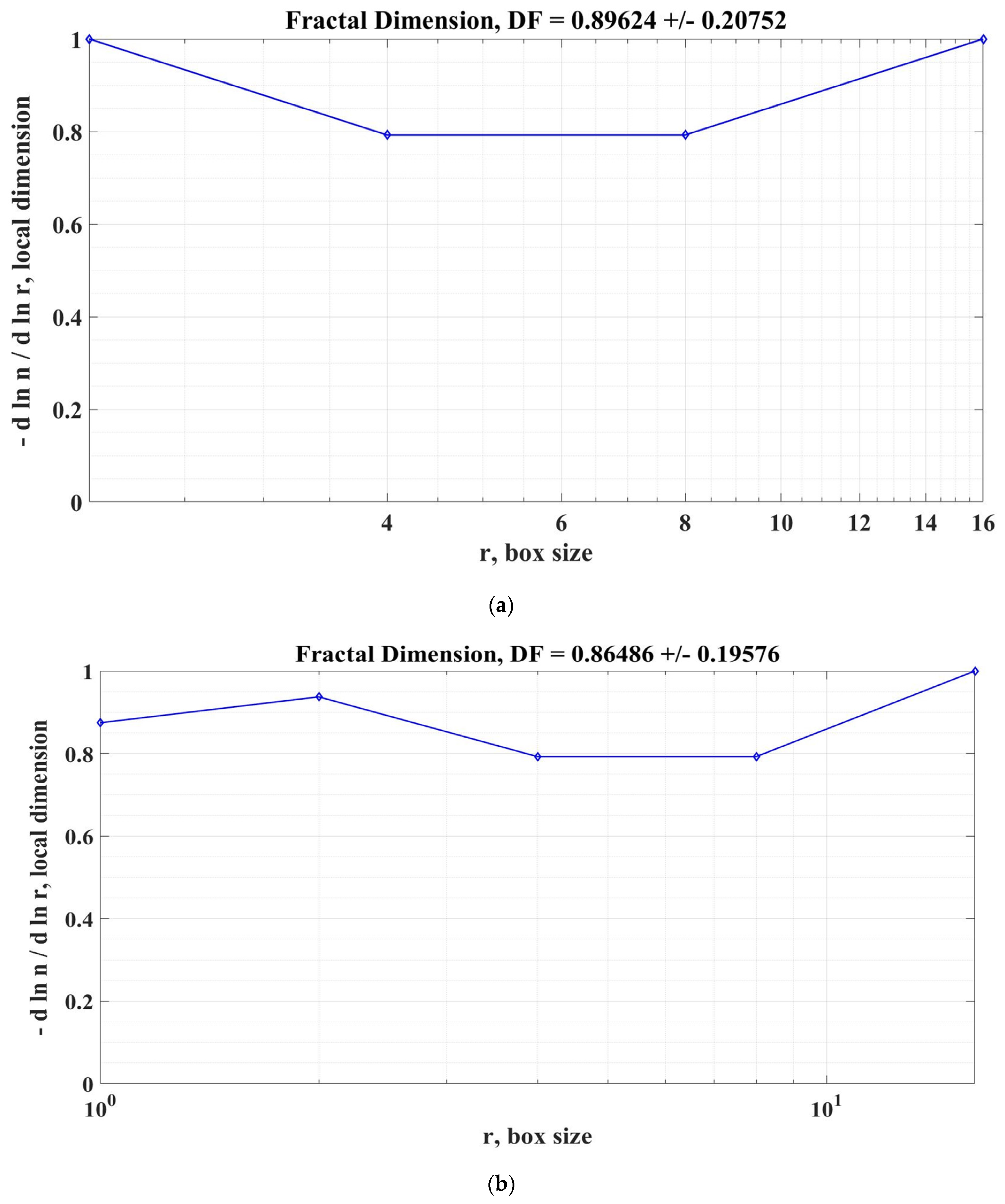
• Implementation in MATLAB/Simulink of the software applications for the calculation of steady-state error, ripple, and DF of the V_DC voltage;
• Implementation in MATLAB/Simulink of the software applications for the calculation of the THD current and voltage on the load side in case of using linear load or nonlinear load (highly polluting in terms of harmonic content).

The rest of the paper is organized as follows: the UPQC system architecture description is presented in Section 2, while the controllers for active power filter and the mathematical description of these controllers is presented in Section 3. Numerical simulations performed in MATLAB/Simulink environment and comparative results of the UPQC-APF control system using the proposed controllers are presented in Section 4. Some conclusions and approaches for future work are presented in Section 5.

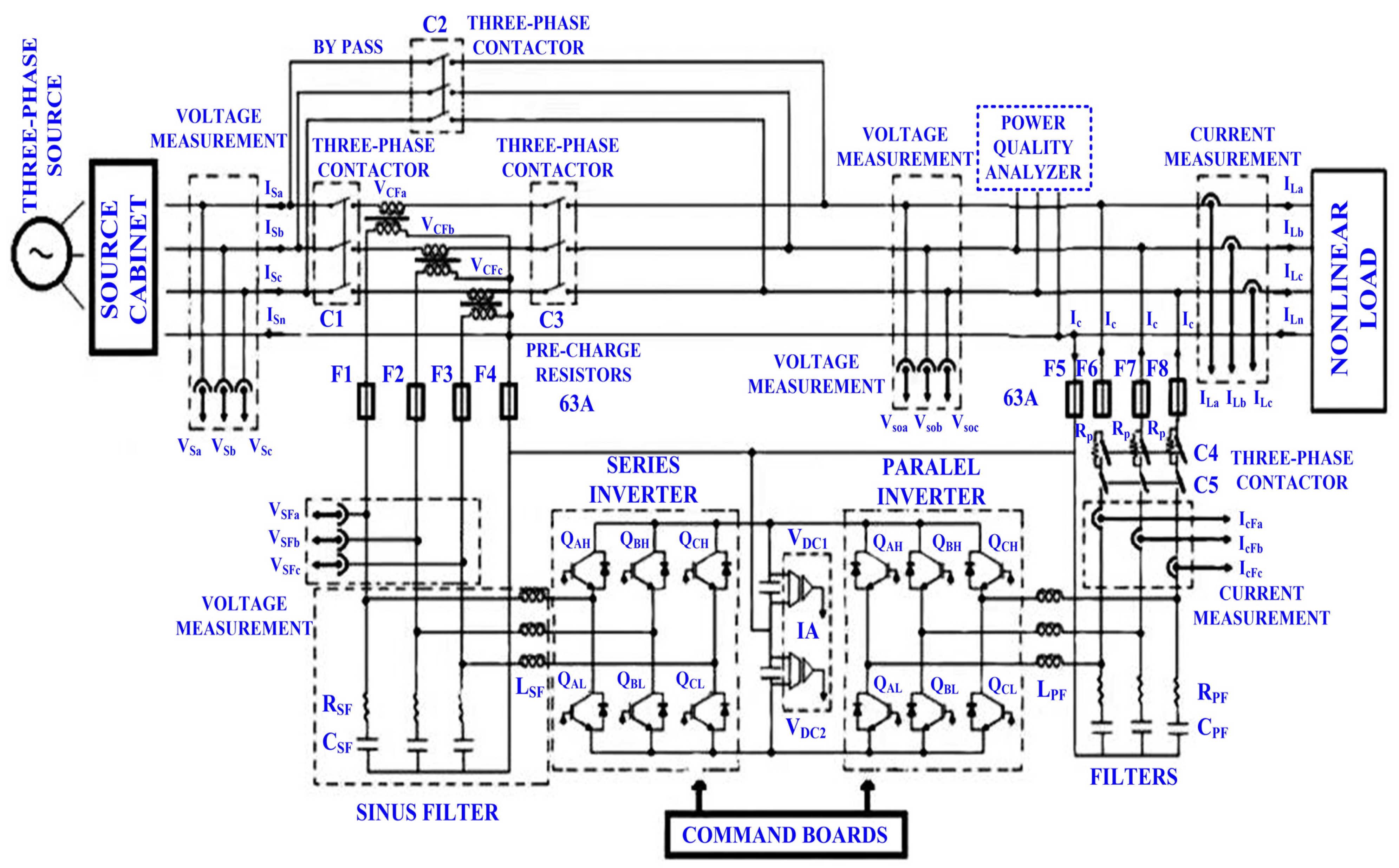
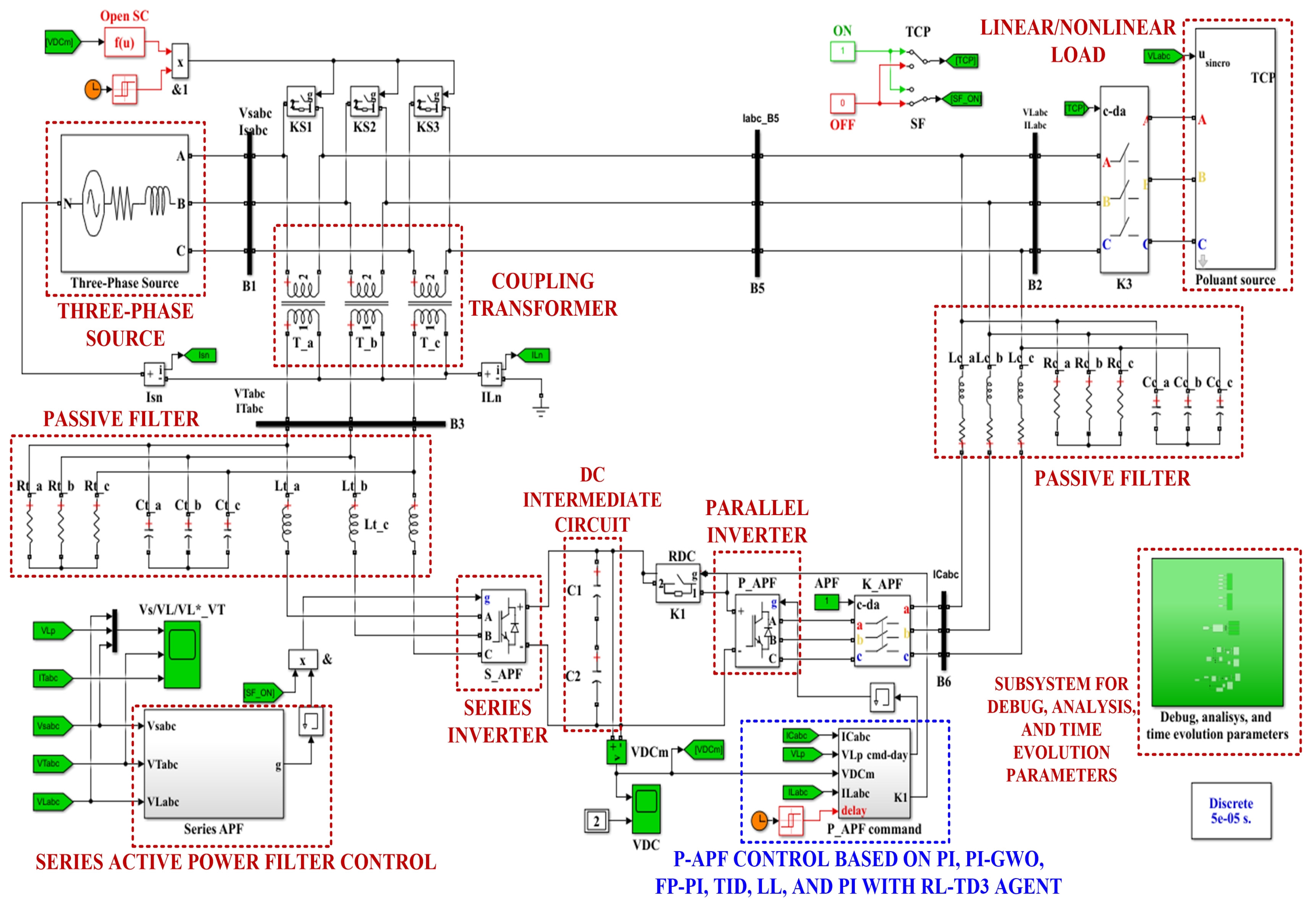
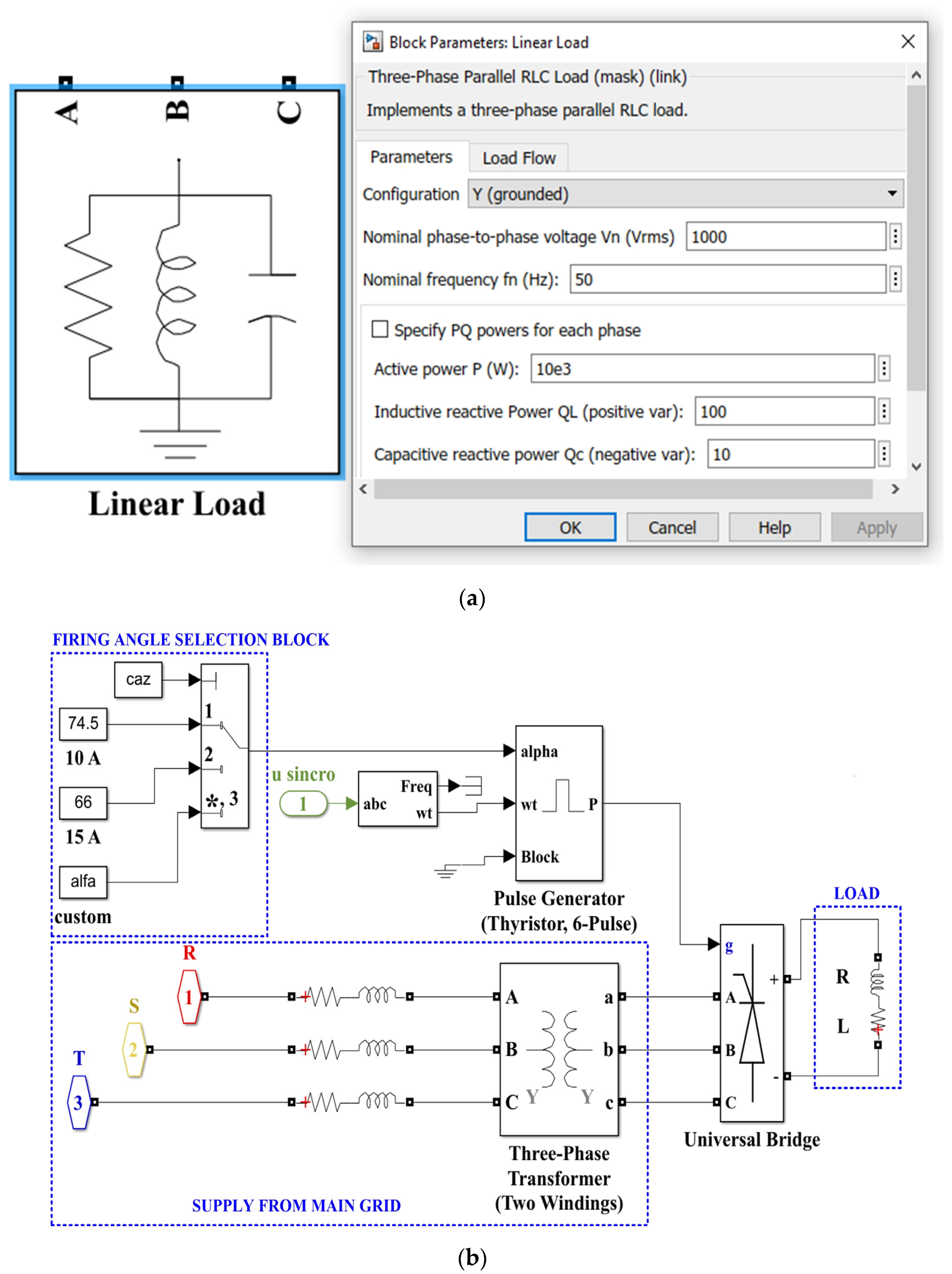
2. UPQC System Description

The UPQC system architecture is shown in Figure 1, and the main components are the common DC intermediate circuit, a series active filter and a parallel active filter. The parallel active filter corrects both the harmonic content introduced by the load and the voltage V_DC in the DC intermediate circuit. The description of the operation starts with the description of the state of contactor C1, located in parallel with the secondary of the transformers in the series filter, and contactor C3 supplying the load. Initially, contactor C1 is closed, and contactor C3 is open. It is necessary to establish these states to ensure the conditions for charging the capacitors in the filter intermediate circuit [25,26].

Since the UPQC system uses high-frequency signals (at least equal to the frequency given by the highest harmonic, which must be compensated) it is necessary to use current and voltage sensors with fast response over a wide range of frequencies and capable of providing galvanic isolation between the power block and the control block.

The general structure of the UPQC adaptive filtering system contains the following main blocks: a series active filter and an APF grouped around a DC intermediate circuit.

The main components of the series active filter can be mentioned: series voltage inverter, coupling transformers, sinusoidal-type filter, contactors for connecting/disconnecting the voltage inverter to the load and for withdrawing the series active filter from the circuit, voltage and current Hall effect transducers. The mains voltage variations and phase voltage unbalances are compensated by the active filter.

Among the components of the parallel active filter, we can mention the following: parallel voltage inverter, mains connection coils, sinusoidal-type filter, current and voltage Hall effect transducers, resistors for limiting the load currents from the DC intermediate circuit of the capacitors, and contactor for connecting/disconnecting the APF to the mains. The main tasks of the APF are as follows: maintaining the constant V_DC voltage in the DC intermediate circuit and attenuating harmonics when using both linear loads and ones that are highly polluting in terms of harmonic content. The DC intermediate circuit is common to both the series active filter, and the APF and includes mainly capacitors that store energy for the operation of these active filters.

In order to reduce THD, the APF will inject into the network currents equal to and 180° out of phase from those causing disturbance in the network, operating in tandem with the active series filter which has high impedance and will be the load for the currents to be compensated. The series active filter controller will provide the V_DC reference voltage for the APF, and the APF controller will provide the I_DC equalizing/balancing current. Obviously, the execution elements controlled by the two active filters will be the Insulated Gate Bipolar Transistor (IGBT) or Metal-Oxide-Semiconductor Field-Effect Transistor (MOSFET) active elements, controlled by PWM signals from the component inverters.

Appendix A presents the main components of the UPQC system hardware implementation.

3. Controllers for Active Power Filter: Mathematical Description

This section presents the main controllers used for the control of the APF presented in the previous section.

3.1. PI Controller

In the time domain, the output of a Proportional Integrator Derivative (PID) controller denoted u(t) as a function of the error e(t), which is defined as the difference between the reference size and the current size can be described like in Equation (1).

Note that by cancelling the derivative component, the PI-type controller used in this paper is obtained.

$$u(t)=K_{p}e(t)+K_i{\displaystyle \underset{0}{\overset{t}{\int }}e(t)}dt+K_d\frac{de(t)}{dt}$$

(1)

In the complex domain s, after applying the Laplace transform, Equation (1) can be written as follows:

$$U(s)=K_{p}E(s)+K_i\frac{1}{s}E(s)+K_{d}sE(s)$$

(2)

In the case of PI controllers, the tuning by using Ziegler–Nichols method is performed like a well-known technique.

3.2. Fractional Order PI Controller

PI^λD^μ-type fractional controllers are described by the following relation [29]:

$$u(t)=K_{p}e(t)+K_i{D}^{-\lambda }e(t)+K_d{D}^{\mu }e(t)$$

(3)

where e(t) represents the signal error.

For the notations in Equation (3), we define the non-integer order operator for integration and differentiation as $a{D}_t^{\alpha }$. The fractional order is denoted as α, and the range limits of the operator are denoted as a and t [29].

$$a{D}_t^{\alpha }=\{\begin{array}{c}\frac{d^{\alpha }}{d{t}^{\alpha }}\mathrm{Re}(\alpha )>0\\ 1\mathrm{Re}(\alpha )=0\\ {\displaystyle {\int }_a^t{(dt)}^{-\alpha }\mathrm{Re}(\alpha )<0}\end{array}$$

(4)

The most commonly used definition for this operator is Riemann–Liouville:

$$a{D}_t^{\alpha }f\left(t\right)=\frac{1}{\Gamma \left(m-\alpha \right)}{\left(\frac{d}{dt}\right)}^m{\displaystyle \underset{\alpha }{\overset{t}{\int }}\frac{f\left(\tau \right)}{{\left(t-\tau \right)}^{\alpha -m+1}}d\tau }$$

(5)

where m − 1 < α < m, $m\in N$, and Euler’s gamma function is denoted by $\Gamma (\cdot )$.

For practical applications, the Grünwald–Letnikov definition is preferred [29]:

$$a{D}_t^{\alpha }f(t)=\underset{h\to 0}{\lim }\frac{1}{h^{\alpha }}{\displaystyle \sum _{j=0}^{\left[\frac{t-\alpha }{h}\right]}{\left(-1\right)}^j}\left(\begin{array}{c}\alpha \\ j\end{array}\right)f\left(t-jh\right)$$

(6)

where [·] represents the integer part.

After applying the Laplace transform to (3) assuming zero initial conditions, the following equation is obtained:

$$G_c(s)=K_p+\frac{K_i}{s^{\lambda }}+K_d{s}^{\mu }$$

(7)

where G_c(s) is the controller’s transfer function, K_p is the proportional factor, K_i is the integral factor, λ is the integrator’s order (positive), K_d is the differential factor, and μ is the differentiator order. For λ = μ = 1, the result is the ordinary integer-order PID controller.

3.3. Fractional Order TID Controller

This controller can be described by the following transfer function [29]:

$$G_c(s)=\frac{K_t}{s^{1/n}}+\frac{K_i}{s}+K_{d}s$$

(8)

where G_c(s) is the controller’s transfer function, K_t is the tilt gain, n is the order of integration of the term tilt, K_i is the amplification factor of the integrator term, and K_d is the amplification factor of the derivative term.

3.4. Fractional Order Lead Lag Controller

The description of this controller can be made as follows [29]:

$$G_c(s)=K_c{\left(\frac{s+\frac{1}{\lambda }}{s+\frac{1}{x\lambda }}\right)}^{\alpha }=K_c{x}^{\alpha }{\left(\frac{\lambda s+1}{x\lambda s+1}\right)}^{\alpha },0<x<1$$

(9)

where G_c(s) is the controller’s transfer function, λ is the fractional order of the FO-Lead-Lag controller.

The lead effect is obtained for α > 0, and the lag effect is obtained for α < 0. The usual form of this type of controller is obtained for $k^{\text{'}}=Kc=x^{\alpha }$.

$$G_c(s)=k^{\text{'}}{\left(\frac{\lambda s+1}{x\lambda s+1}\right)}^{\alpha }$$

(10)

For $k^{\text{'}}=\alpha =1$, $\lambda =\frac{K_p}{K_i}$, and x has a very large value (e.g., x > 10,000), so the FO-Lead-Lag controller transfer function becomes similar to the FO-PI controller transfer function.

3.5. Optimization of PI Controller Using GWO Algorithm

A GWO algorithm can be used to choose the parameters K_p and K_i of the PI controllers described by Equations (1) and (2) in order to optimize the performance of the closed-loop control loop.

It can be described using the way the grey wolf hunts in groups to catch prey. The leading wolf is denoted by α, and the second most important wolf by β. The third most important wolf in the group is denoted by δ, and the wolf with the least importance in the group is denoted by ω. The four steps, search for prey, encircle prey, attack and hunt prey, form the starting point of the GWO algorithm analogy.

After generating the initial positions of the wolves and their initial positions, by denoting the position of the prey as X_n(k) and the position of a wolf at the current iteration as X(k), the following equations can be written [27]:

$$D=\left|C{X}_p(k)-X(k)\right|$$

(11)

$$X(k+1)=X_p(k)-AD$$

(12)

where k is the iterations number, and D is the new position of the grey wolf. A and C are denoted as $A=2a{r}_1-a,r_1\in [0,1]$ and $C=2a{r}_2,r\in 2[0,1]$ where the parameter a has a linear decrease between 2 and 0.

By denoting the position of a wolf at each iteration as (x, y), and the position of the location of the prey as $\left(x^{\prime },y^{\prime }\right)$ the following relations can be written [27]:

$$D_{\alpha }=\left|C_1{X}_{\alpha }(k)-X(k)\right|$$

(13)

$$D_{\beta }=\left|C_2{X}_{\beta }(k)-X(k)\right|$$

(14)

$$D_{\delta }=\left|C_3{X}_{\delta }(k)-X(k)\right|$$

(15)

$$X_1=X_{\alpha }-A_1{D}_{\alpha }$$

(16)

$$X_2=X_{\beta }-A_2{D}_{\beta }$$

(17)

$$X_3=X_{\delta }-A_3{D}_{\delta }$$

(18)

$$X(k+1)=\frac{X_1+X_2+X_3}{3}$$

(19)

The GWO algorithm, when used to determine the optimal K_p and K_i values of the PI controller for the control of the APF, is completed after a proposed maximum number of iterations or after the minimum of the objective function has been reached with a required accuracy. Usually, the objective function is defined as an integral criterion of the squared error and characterizes the overall performance of the control system.

3.6. Improvement Performances of PI Controller Using RL-TD3 Agent

Generally speaking, RL is about the computer learning to execute a task when it interacts dynamically with an unknown process. Without explicitly programming the manner of learning the task, the learning process is based on a set of decisions that are made, so as to maximize the cumulative reward, whose expression is established in advance [23,24].

Figure 2 shows the block diagram of an RL scenario for use in the process control.

The input signals to the agent are observation and reward. The observation consists of a set of predefined signals that characterize the process, and the reward is defined as a measure of the success of the action output signal. The action is represented by the control inputs of the controlled process. Observations represent the signals visible to the agent and are in the form of measured signals, their rate of change and the associated errors. Usually, the reward is formed as part of the continuous actions as a sum of the square of the error of the signals of interest and the square of the past actions. These terms are given a weight set by the final goal of the problem. In the process control, the reward is given by a function that implements stationary error minimization [23,24].

The reward at each step for this case is given by the following relation:

$$r_{\mathrm{int}}=-\left(Q\cdot V_{DCerror}^2+R{\displaystyle \sum _j{\left(u_{t-1}^j\right)}^2}\right)$$

(20)

where usually, the parameter values Q = 0.5 and R = 0.1, and $u_{t-1}^j$ are the actions from the previous step.

It should be noted that of the machine learning types, the RL-TD3 agent has a similar operation to the control of an industrial process. Thus, it reads the inputs, calculates the reward, which is analogous to an integral performance criterion (in Equation (20), this is given by a discrete form), and generates outputs analogous to the control inputs. After the training phase of the RL-TD3 agent, it provides additional correction signals that are added to the PI controller outputs to improve the performance of the APF control system.

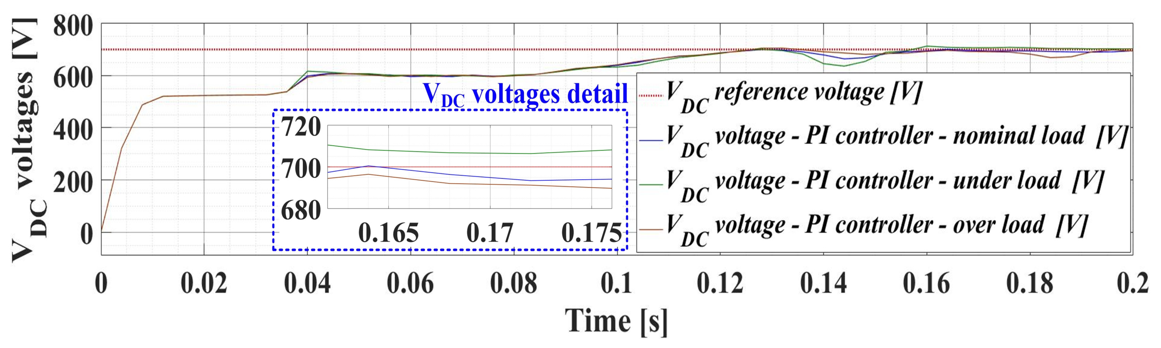
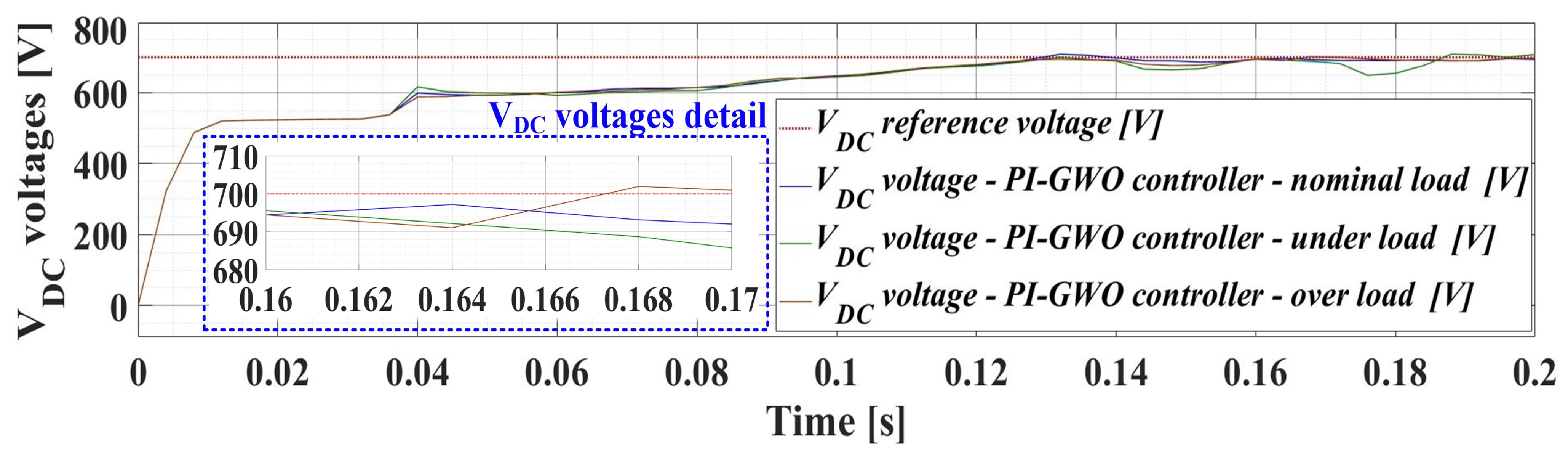
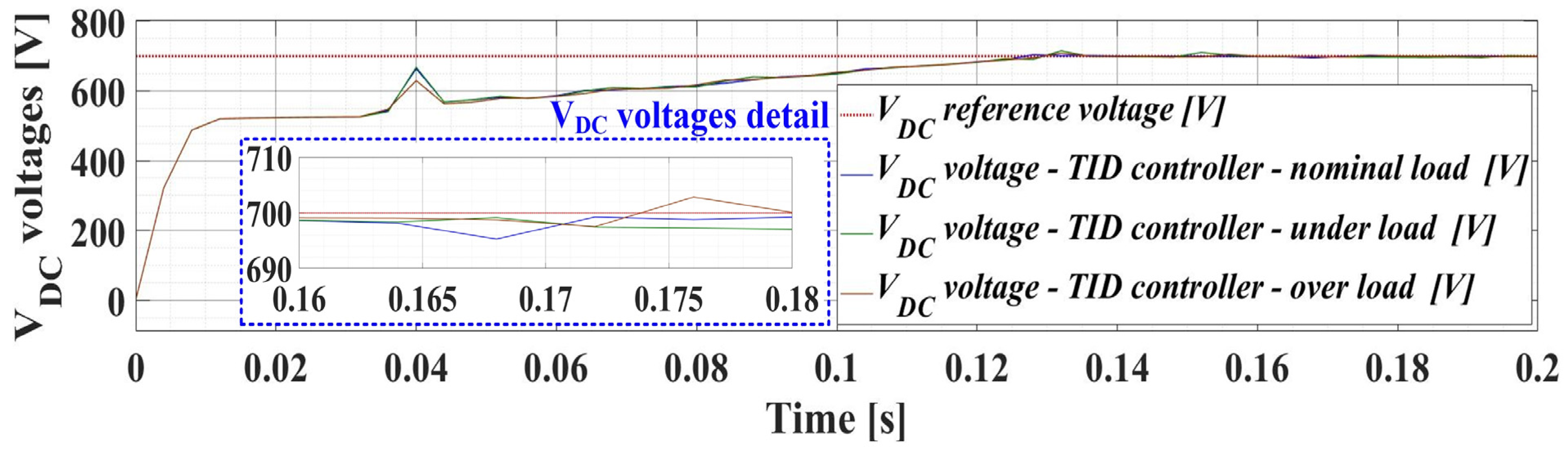
4. Numerical Simulations

In this section, the performance of the APF control system will be compared through numerical simulations using the MATLAB/Simulink environment. The intended quality goals are to maintain the lowest error and ripple of the V_DC voltage of the DC intermediate circuit, presented in Figure 3, and also the lowest current and voltage THD, both in the case of a usual linear load and in the case of a nonlinear load that is highly polluting in terms of harmonic content.

Among UPQC system components, we can mention the following blocks used in MATLAB/Simulink implementation: three-phase source block; passive filters blocks; active series filter and APF control subsystems; series and parallel inverters block; coupling transformer blocks; DC intermediate circuit block; nonlinear/linear load subsystem (Figure 4a,b); switches and breakers blocks; debug, analysis, and time evolution for the UPQC system parameters subsystem. The nonlinear load consists of a controlled inverter which consist in an RL series circuit at the output, with a resistance of value R = 4 Ω and an inductance of value L = 35 mH. Thus, the main role of the UPQC system is to improve the power quality on both sides the source and the load. Usually, the subsystem for controlling active filters is based on classical PI controllers.

In addition to the description of the UPQC system operation, it should be noted that the charging of the intermediate circuit capacitors is carried out in three stages:

• In the first stage, to limit the charging current, contactor K1 (short-circuiting the RDC resistor) is opened. When the voltage on the capacitors reaches 480 V, the second stage starts;
• In the second stage, the capacitors continue to charge directly, without driving the parallel filter elements. This stage continues until the voltage on the capacitors reaches 525 V. The two thresholds (480 V and 525 V, respectively) have been set through testing to ensure a reasonable dynamic charging rate. They can be set to different values;
• In the third stage, the parallel filter transistors start to be controlled.

By replacing the PI controller normally tuned (empirically or by using the Ziegler–Nichols method) with a PI controller optimally tuned using the GWO algorithm or FO-PI controller, TID controller, Lead-Lag controller (Figure 5), PI controller with RL-TD3 agent (Figure 6), superior performances are obtained. One of the important performances is to maintain a constant value (V_DC = 700 V) of the voltage, with a ripple as small as possible in the common DC circuit for the two series and parallel inverters.

After tuning the PI, PI-GWO, and FO-PI controllers according to the methods presented above in Section 3.1, 3.2 and 3.5, the values presented in

Table 1. Tuned parameters of PI, PI-GWO, and FO-PI controllers.

Controller	Parameter Kp	Parameter Ki	Parameter λ
PI	0.1	0.1	–
PI-GWO	0.18	39.51	–
FO-PI	2.38	0.85	0.73

are obtained.

Following the elements presented in Section 3.3 for the TID controller the following parameters were chosen: K_t = 1.2, K_i = 12, n = 10, and K_d = 0. Thus, the following FO-type controller is obtained in the form of the TID controller transfer function:

$$H_{TID}=\frac{1.2+12s^{0.1}}{s^{1.1}}$$

(21)

Following the elements presented in Section 3.4 for the FO-Lead-Lag controller the following parameters were chosen: $k\text{'}=300$, x = 50, λ = 1.4, and α = 0.11. Thus, the following FO-type controller is obtained in the form of the FO-Lead-Lag controller transfer function:

$$H_{LL}=\frac{3.606\cdot {10}^8}{s^{2.1}+7.373\cdot {10}^4{s}^{1.1}+4.74\cdot {10}^6}$$

(22)

Appendix B presents a series of notions regarding the method of implementation of the real-time FO controllers in embedded systems.

Following the elements presented in Section 3.6, the result of the performance of the 200 epochs RL-TD3 agent drive is presented in Figure 7.

Following the numerical simulations, comparative results were obtained for the time evolution of the V_DC voltage for each of the controllers presented for the APF control when the nonlinear load can be nominal load, under load, and over load, respectively. Note that the load resistance values in this case are 4Ω, 3Ω, and 5Ω, respectively.

Thus, Figure 8 shows the V_DC voltage evolution in the DC intermediate circuit when using a PI controller for APF control, while Figure 9 shows the same quantities of interest for APF control using a PI-GWO controller. Furthermore, Figure 10, Figure 11 and Figure 12 show the V_DC voltage evolution for APF control using FO-type controllers is shown, namely, FO-PI, TID, and FO-Lead-Lag, respectively. In the case of using an RL-TD3 agent in tandem with a PI controller for APF control, Figure 13 shows the V_DC voltage evolution.

In the case of the nominal nonlinear load, Figure 14 compares the V_DC voltage evolution in the DC intermediate circuit when using the six types of controllers: PI, PI-GWO, FO-PI, TID, and FO-Lead-Lag controllers, as well as the PI controller with the RL-TD3 agent for correction of command signals.

Table 2. Performance indicators of the V_DC voltage control for UPQC-APF control system based on the presented controllers.

Controller	Stationary Error [%]	Voltage Ripple [V]	DF
PI	1	145.71	0.79248 +/− 0.17540
PI-GWO	0.50	143.76	0.83048 +/− 0.20534
FO-PI	0.41	142.92	0.83048 +/− 0.20534
TID	0.30	142.15	0.86486 +/− 0.19576
FO-Lead-Lag	0.25	141.82	0.86486 +/− 0.19576
PI with RL-TD3 agent	0.10	141.11	0.89624 +/− 0.20752

shows the performance indicators of the UPQC-APF control system based on PI controller, PI-GWO controller, FO-PI controller, TID controller, FO-Lead-Lag controller, and PI controller with RL-TD3 agent for correction of command signals. These performance indicators are as follows: stationary error, voltage ripple, and DF.

Voltage ripple is defined as follows [23]:

$$V_{DCripple}=\sqrt{\frac{1}{N}{\displaystyle \sum _{i=1}^N{\left(V_{DC}(i)-V_{DCref}(i)\right)}^2}}$$

(23)

where the number of samples is denoted as N, V_DC represents the voltage in DC intermediate circuit, and the reference voltage is denoted as V_DCref = 700 V.

Improved performance of the PI controllers is noted when optimizing the tuning parameters by a GWO computational intelligence method. Additionally, better performance is obtained when using FO controllers: FO-PI controller, TID controller, and FO-Lead-Lag controller. This can be explained by the fact that we have an additional degree of freedom in tuning FO controllers, namely, the FO. The best results for APF control were obtained by using the PI-type controller combined with the RL-TD3 agent, due to the fact that after training, the RL-TD3 agent will provide correction signals, following the optimization of a performance criterion, which will overlap the commands of the basic PI-type controller.

The analysis of some electrical signals in an inverter-plus-load circuit is presented in [31], where it is shown that the better the inverter control (achieved by various types of controlled/uncontrolled sources) the more DF of the electrical signals increases. Thus, for the system presented in this article, following the use of the controllers presented in the previous section, in addition to the stationary error and the V_DC voltage ripple, the DF of these voltage signals is also analyzed for the V_DC voltage signals.

The following briefly describes the method of calculating the DF of a signal, in the case of our application, a one-dimensional signal. For this, we use the box-counting method. Thus, for the analyzed one-dimensional signal, we find a square that encompasses all of it, in which the length of one side is considered the unit of measurement. The chosen square must contain all the non-zero values of the signal, and the size chosen for the scale is preferable to be power of 2 for quick calculation.

In addition, the unit of measurement is repeatedly divided by 2 until the value obtained decreases below a predefined threshold. This form of division is of the form 1/2k, where k represents the current step. On the other axis, the division is of the form $\frac{n_k}{2^{2k}}$, where n_k represents the total number of domains that are occupied by the signal at the given scale.

For each sequence at the current step, the values obtained on the two axes following the procedure described above can be considered as the coordinates of a point M_k(x,y), and the representation is in the Cartesian system but with log coordinates. Using these values, the coordinates of the sequences of points M₁, M₂, ..., M_n are calculated sequentially at each step k (until reaching values over the chosen threshold). The slope of the line closest to the points M₁, M₂, ..., M_n, provides the DF of the initial signal. Using the following MATLAB command “[n,r] = boxcount(signal,’slope’)” the vectors corresponding to the two dimensions in the algorithm described above are obtained.

With the following MATLAB commands: “df = −diff(log(n))./diff(log(r))” and “[‘DF = ‘num2str(mean(df(1:length(df)))) ‘+/− ‘num2str(std(df(1:length(df))))])” the coordinates of the points Mk and the slope of the line closest to the points M₁, M₂, ..., M_n, i.e., DF are obtained in logarithmic coordinates [31].

Figure 15 shows the DF calculation for the V_DC voltage signal when using the controllers shown in the previous section. It can be noted that DF is maximum for the PI controller with RL-TD3 agent and minimum for the PI controller. It is also noted that for PI-GWO- and FO-PI-type controllers, the same DF is obtained, and the same is noted for TID- and FO-Lead-Lag-type controllers. It can therefore be noted that the claim made in [31], namely, that DF is higher for a more efficient controller, is verified.

Additionally, by analyzing Table 2, we can notice the high values for the ripple and stationary error of V_DC voltage corresponding to the use of the PI controller and the PI controller with RL-TD3 agent, respectively, while the values of these two indicators are relatively close when using PI-GWO and FO-PI controllers on the one hand and when using TID and FO-Lead-Lag controllers on the other hand. Therefore, there is conformity with the DF obtained for the V_DC voltage signal for the six types of controllers compared.

Another important indicator of the performance of an APF in a UPQC-type system is the THD. Both THD current and THD voltage for the most efficient (PI controller with RL-TD3 agent) and the least efficient (PI controller) of the presented controllers will be presented by FFT analysis. For this, both a nonlinear load presented above which is highly polluting in terms of harmonics, containing switching elements but no filters, and a 100 kW/10 Kvar RLC linear load are considered.

THD current is described by the next expression [32]:

$$THD(\%)=\frac{\sqrt{{\displaystyle \sum _{n=1}^N{I}_N^2}}}{I_{RMS}}$$

(24)

where I_N represents the RMS value of the harmonic N and I_RMS represents RMS value of the fundamental of the signal.

The THD voltage is defined in a similar way. Thus, Figure 16a,b show the FFT and THD current analysis for a PI-type controller under a nonlinear and a linear load, respectively. Similarly, Figure 16c,d show the FFT and THD current analysis for a PI controller with RL-TD3 agent under a nonlinear and a linear load, , respectively. A decrease in the THD current value from 22.82% to 16.71% is noted in the worst case. Regarding the THD analysis in terms of voltage, for the combinations of controllers and loads presented above, the results obtained are shown in Figure 17. There is a decrease in THD voltage from 2.04% in the worst case to 0.18%. It can be concluded that the order of the performance of the presented controllers is also consistent with the performances shown in Table 2 in the case of current or voltage THD analysis.

5. Conclusions

This article presents the general architecture of a UPQC, whose main components are the common DC circuit, a series active filter and an APF. The parallel active filter corrects both the harmonic content introduced by the load and the DC voltage V_DC in the DC intermediate circuit. Thus, starting from the performance of a PI-type controller integrated in the UPQC-APF control system, the performance is compared for more complex controllers such as: PI controller optimally tuned using the GWO algorithm, FO-PI controller, TID controller, FO-Lead-Lag controller, and PI controller with RL-TD3 agent. The main performance indicators of the UPQC-APF control system for the controllers listed above are: stationary error of V_DC voltage, ripple of V_DC voltage, and DF of V_DC voltage. Results are also presented on the improvement of both current and voltage THD in the case of, respectively, a linear and nonlinear load heavily polluting in terms of harmonic content. Numerical simulations carried out in MATLAB/Simulink environment demonstrate the superior performance of UPQC-APF control system when using PI with RL-TD3 agent and FO-type controllers compared to classical PI controllers. This can be explained by the fact that the RL-TD3 agent provides additional correction signals that are added to the PI controller outputs to improve the performance of the UPQC-APF control system. In the case of FO, the explanation of the superiority of these types of controllers over the classic PI type resides in the existence of an additional tuning parameter. In [25,26], the implementation of classical PI and integer order algorithms in an embedded system is presented, and following the elements presented in Appendix A and Appendix B, the implementation of FO control algorithms in real time in embedded systems will be presented in future papers.

References

1. Honarmand, M.E.; Hosseinnezhad, V.; Hayes, B.; Siano, P. Local Energy Trading in Future Distribution Systems. Energies 2021, 14, 3110. [Google Scholar] [CrossRef]
2. Chartier, S.L.; Venkiteswaran, V.K.; Rangarajan, S.S.; Collins, E.R.; Senjyu, T. Microgrid Emergence, Integration, and Influence on the Future Energy Generation Equilibrium—A Review. Electronics 2022, 11, 791. [Google Scholar] [CrossRef]
3. Ayalew, M.; Khan, B.; Giday, I.; Mahela, O.P.; Khosravy, M.; Gupta, N.; Senjyu, T. Integration of Renewable Based Distributed Generation for Distribution Network Expansion Planning. Energies 2022, 15, 1378. [Google Scholar] [CrossRef]
4. Nafkha-Tayari, W.; Ben Elghali, S.; Heydarian-Forushani, E.; Benbouzid, M. Virtual Power Plants Optimization Issue: A Comprehensive Review on Methods, Solutions, and Prospects. Energies 2022, 15, 3607. [Google Scholar] [CrossRef]
5. Maciążek, M. Active Power Filters and Power Quality. Energies 2022, 15, 8483. [Google Scholar] [CrossRef]
6. Buła, D.; Grabowski, D.; Maciążek, M. A Review on Optimization of Active Power Filter Placement and Sizing Methods. Energies 2022, 15, 1175. [Google Scholar] [CrossRef]
7. Yang, B.; Liu, K.; Zhang, S.; Zhao, J. Design and Implementation of Novel Multi-Converter-Based Unified Power Quality Conditioner for Low-Voltage High-Current Distribution System. Energies 2018, 11, 3150. [Google Scholar] [CrossRef] [Green Version]
8. Sekhar, A.H.; Bharathi, S.L.K.; Asif, N.A.H.; Manikandan, P.V. Power Quality Enhancement Using Multi-Level Inverter with UPQC and Robust Back Propagation Neural Network Strategy. SPAST Abstr. 2021, 1. Available online: https://spast.org/techrep/article/view/2967 (accessed on 10 June 2022). [CrossRef]
9. Gupta, A. Power quality evaluation of photovoltaic grid interfaced cascaded H-bridge nine-level multilevel inverter systems using D-STATCOM and UPQC. Energy 2022, 238, 121707. [Google Scholar] [CrossRef]
10. Mahdi, D.I.; Gorel, G. Design and Control of Three-Phase Power System with Wind Power Using Unified Power Quality Conditioner. Energies 2022, 15, 7074. [Google Scholar] [CrossRef]
11. Yang, D.; Ma, Z.; Gao, X.; Ma, Z.; Cui, E. Control Strategy of Intergrated Photovoltaic-UPQC System for DC-Bus Voltage Stability and Voltage Sags Compensation. Energies 2019, 12, 4009. [Google Scholar] [CrossRef] [Green Version]
12. Garces-Gomez, Y.A.; Hoyos, F.E.; Candelo-Becerra, J.E. Classic Discrete Control Technique and 3D-SVPWM Applied to a Dual Unified Power Quality Conditioner. Appl. Sci. 2019, 9, 5087. [Google Scholar] [CrossRef] [Green Version]
13. Afonso, J.L.; Tanta, M.; Pinto, J.G.O.; Monteiro, L.F.C.; Machado, L.; Sousa, T.J.C.; Monteiro, V. A Review on Power Electronics Technologies for Power Quality Improvement. Energies 2021, 14, 8585. [Google Scholar] [CrossRef]
14. Das, S.R.; Ray, P.K.; Sahoo, A.K.; Ramasubbareddy, S.; Babu, T.S.; Kumar, N.M.; Elavarasan, R.M.; Mihet-Popa, L. A Comprehensive Survey on Different Control Strategies and Applications of Active Power Filters for Power Quality Improvement. Energies 2021, 14, 4589. [Google Scholar] [CrossRef]
15. El Ghaly, A.; Tarnini, M.; Moubayed, N.; Chahine, K. A Filter-Less Time-Domain Method for Reference Signal Extraction in Shunt Active Power Filters. Energies 2022, 15, 5568. [Google Scholar] [CrossRef]
16. Kołek, K.; Firlit, A. A New Optimal Current Controller for a Three-Phase Shunt Active Power Filter Based on Karush–Kuhn–Tucker Conditions. Energies 2021, 14, 6381. [Google Scholar] [CrossRef]
17. Buła, D.; Grabowski, D.; Lewandowski, M.; Maciążek, M.; Piwowar, A. Software Solution for Modeling, Sizing, and Allocation of Active Power Filters in Distribution Networks. Energies 2021, 14, 133. [Google Scholar] [CrossRef]
18. Kenjrawy, H.; Makdisie, C.; Houssamo, I.; Mohammed, N. New Modulation Technique in Smart Grid Interfaced Multilevel UPQC-PV Controlled via Fuzzy Logic Controller. Electronics 2022, 11, 919. [Google Scholar] [CrossRef]
19. Mahar, H.; Munir, H.M.; Soomro, J.B.; Akhtar, F.; Hussain, R.; Elnaggar, M.F.; Kamel, S.; Guerrero, J.M. Implementation of ANN Controller Based UPQC Integrated with Microgrid. Mathematics 2022, 10, 1989. [Google Scholar] [CrossRef]
20. Mota, D.d.S.; Tedeschi, E. On Adaptive Moving Average Algorithms for the Application of the Conservative Power Theory in Systems with Variable Frequency. Energies 2021, 14, 1201. [Google Scholar] [CrossRef]
21. Karchi, N.; Kulkarni, D.; Pérez de Prado, R.; Divakarachari, P.B.; Patil, S.N.; Desai, V. Adaptive Least Mean Square Controller for Power Quality Enhancement in Solar Photovoltaic System. Energies 2022, 15, 8909. [Google Scholar] [CrossRef]
22. Gaburro Bacheti, G.; Sartório Camargo, R.; Silva Amorim, T.; Yahyaoui, I.; Frizera Encarnação, L. Model-Based Predictive Control with Graph Theory Approach Applied to Multilevel Back-to-Back Cascaded H-Bridge Converters. Electronics 2022, 11, 1711. [Google Scholar] [CrossRef]
23. Nicola, M.; Nicola, C.-I. Improved Performance in the Control of DC-DC Three-Phase Power Electronic Converter Using Fractional-Order SMC and Synergetic Controllers and RL-TD3 Agent. Fractal Fract. 2022, 6, 729. [Google Scholar] [CrossRef]
24. Nicola, M.; Nicola, C.-I. Comparative Performance Analysis of the DC-AC Converter Control System Based on Linear Robust or Nonlinear PCH Controllers and Reinforcement Learning Agent. Sensors 2022, 22, 9535. [Google Scholar] [CrossRef] [PubMed]
25. Nicola, M.; Sacerdoțianu, D.; Nicola, C.-I.; Ivanov, S.; Ciontu, M.; Nițu, M.-C. Improved Control Strategy of Unified Power Quality Conditioner Using Fractional Order Controller and Particle Swarm Optimization. In Proceedings of the International Conference on Applied and Theoretical Electricity (ICATE), Craiova, Romania, 27–29 May 2021; pp. 1–6. [Google Scholar]
26. Ivanov, S.; Ciontu, M.; Sacerdoțianu, D.; Radu, A. Simple control strategies of the active filters within a unified power quality conditioner (UPQC). In Proceedings of the International Conference on Modern Power Systems (MPS), Cluj-Napoca, Romania, 6–9 June 2017; pp. 1–4. [Google Scholar]
27. Zychlewicz, M.; Stanislawski, R.; Kaminski, M. Grey Wolf Optimizer in Design Process of the Recurrent Wavelet Neural Controller Applied for Two-Mass System. Electronics 2022, 11, 177. [Google Scholar] [CrossRef]
28. Benbouhenni, H.; Bizon, N.; Colak, I.; Thounthong, P.; Takorabet, N. Application of Fractional-Order PI Controllers and Neuro-Fuzzy PWM Technique to Multi-Rotor Wind Turbine Systems. Electronics 2022, 11, 1340. [Google Scholar] [CrossRef]
29. Tepljakov, A.; Petlenkov, E.; Belikov, J. Closed-loop identification of fractional-order models using FOMCON toolbox for MATLAB. In Proceedings of the 14th Biennial Baltic Electronic Conference (BEC), Tallinn, Estonia, 6–8 October 2014; pp. 213–216. [Google Scholar]
30. Faria, R.d.R.; Capron, B.D.O.; Secchi, A.R.; de Souza, M.B., Jr. Where Reinforcement Learning Meets Process Control: Review and Guidelines. Processes 2022, 10, 2311. [Google Scholar] [CrossRef]
31. Voncilă, I.; Selim, E.; Voncilă, M.-L. Use of fractal analysis for quality evaluation of control methods in induction motor drive systems. In Proceedings of the 6th International Conference on System Theory, Control and Computing (ICSTCC), Sinaia, Romania, 19–21 October 2022; pp. 524–529. [Google Scholar]
32. IEEE Std 1159-2019; IEEE Recommended Practice for Monitoring Electric Power Quality. Institute of Electrical and Electronics Engineers: New York, NY, USA, 2019.
Figure 1. UPQC system architecture [25].
Electronics 12 00494 g001
Figure 2. Block diagram of an RL scenario for use in the process control.
Electronics 12 00494 g002
Figure 3. MATLAB/Simulink implementation of the UPQC system.
Electronics 12 00494 g003
Figure 4. Load types: (a) linear load; (b) nonlinear load.
Electronics 12 00494 g004
Figure 5. Block diagram subsystem implementation in MATLAB/Simulink of the APF control system based on PI, PI-GWO, FO-PI, TID, and FO-Lead-Lag controllers.
Electronics 12 00494 g005
Figure 6. Block diagram subsystem implementation in MATLAB/Simulink of the APF control system based on PI controller with RL-TD3 agent.
Electronics 12 00494 g006
Figure 7. Performance of the RL-TD3 algorithm based on reward evolution.
Electronics 12 00494 g007
Figure 8. VDC voltages time evolution of the UPQC-APF control system based on PI controller in case of nonlinear load.
Electronics 12 00494 g008
Figure 9. VDC voltages time evolution of the UPQC-APF control system based on PI-GWO controller in case of nonlinear load.
Electronics 12 00494 g009
Figure 10. VDC voltages time evolution of the UPQC-APF control system based on FO-PI controller in case of nonlinear load.
Electronics 12 00494 g010
Figure 11. VDC voltages time evolution of the UPQC-APF control system based on TID controller in case of nonlinear load.
Electronics 12 00494 g011
Figure 12. VDC voltages time evolution of the UPQC-APF control system based on FO-Lead-Lag controller in case of nonlinear load.
Electronics 12 00494 g012
Figure 13. VDC voltages time evolution of the UPQC-APF control system based on PI controller with RL-TD3 agent in case of nonlinear load.
Electronics 12 00494 g013
Figure 14. VDC voltages time evolution comparison of the UPQC-APF control system based on presented controllers in case of nominal nonlinear load.
Electronics 12 00494 g014
Figure 15. DF of VDC voltage signal in case of the following controller type: (a) PI controller with RL-TD3 agent; (b) TID and FO-Lead-Lag controllers; (c) FO-PI and PI-GWO controllers; (d) PI controller.
Electronics 12 00494 g015aElectronics 12 00494 g015b
Figure 16. FFT analysis and THD current calculus for APF control: (a) PI controller and nonlinear load; (b) PI controller and linear load; (c) PI controller with RL-TD3 agent and nonlinear load; (d) PI controller with RL-TD3 agent and linear load.
Electronics 12 00494 g016
Figure 17. FFT analysis and THD voltage calculus for APF control: (a) PI controller and nonlinear load; (b) PI controller and linear load; (c) PI controller with RL-TD3 agent and nonlinear load; (d) PI controller with RL-TD3 agent and linear load.
Electronics 12 00494 g017