
A Novel Image Encryption Algorithm Based on Multiple Random DNA Coding and Annealing

Abstract
:1. Introduction
- (1)
- The idea that image processing can be done using chaotic pixel random variation is proposed for the first time. An increase of the variety of texture and encryption coding methods can be achieved by using Logistic-Logistic Chaos (LLC), which provides a greater range of parameter selection and better randomness.
- (2)
- The randomness and security of the coding process are improved by randomly selecting multiple DNA coding methodologies, as well as codes that operate on them, for each variant pixel.
- (3)
- Various weights are assigned to the information entropy, pixel correlation, and for annealing iteration, resulting in different encryption processes and good encryption results of different images based on the pixel variation, scrambling, and diffusion stages.
2. Preliminaries
2.1. Chaotic System
2.2. Pixel Random Variation(PRV)
2.3. Multiple Random DNA Coding Diffusion(MRDD)
3. Multi-D&A Image Encryption Algorithm
3.1. Annealing Process for Encryption(APE)
- (1)
- Utilize a function method to transform the current solution into a new one.
- (2)
- Calculate the difference between the current and updated solutions by substituting them into the target function.
- (3)
- Use the Metropolis criterion to determine whether the new solution can replace the current solution. , where S and S’ are two solutions, is the increment, and is the target function. If , the new solution is accepted, otherwise, the probability of accepting the new solution is , where is the parameter changing over time.
- (4)
- A further iteration is carried out until the final solution has been reached.
3.2. Detailed Steps for Encryption
3.3. Decryption Procedure
| Algorithm 1. Decryption procedure |
| Input: Ciphertext image I sized to m × n; Initial value; Sequence |
| pseudo random number sequence (i) of length m × n, (i)∈{0,1,...,9} |
| Output: Decrypted image image |
| Use to generate pseudo random number sequence S(i) of length 1000 + m × n × 8. |
| for j = 1 to 200: |
| if (j) = 1 |
| I = MRDD(I); |
| I2 = I; |
| else |
| I2 = I; |
| end |
| Algorithm 2. PRV |
| Input: image I sized to m × n |
| pseudo random number sequence (i) of length m × n, (i)∈{0,1,...,9} |
| Output: image after random pixel change |
| Convert image I into a one-dimensional sequence of length m × n |
| for j = 1 to m × n: |
| Convert pixel (j) to 8-bit binary B |
| if S(j)∈{1,...,8} |
| Invert the (j)-th bit of B to obtain |
| else |
| Invert all bits of B to obtain |
| end |
| (j) = |
| end |
| Converts the sequence into an image of size m × n |
| Algorithm 3. MRDD |
| Input: image I sized to m × n |
| pseudo random number sequence (i) of length m × n, (i)∈{1,...,8} |
| pseudo random number sequence (i) of length m × n, (i)∈{0,...,255} |
| pseudo random number sequence (i) of length m × n, (i)∈{1,...,8} |
| pseudo random number sequence (i) of length m × n, (i)∈{1,2,3,4} |
| pseudo random number sequence (i) of length m × n, (i)∈{1,...,8} |
| Output: diffused image |
| Convert image I into a one-dimensional sequence of length m × n |
| for j = 1 to m × n: |
| Encode (j) according to DNA coding rule (j) to obtain |
| Encode (j) according to DNA coding rule (j) to obtain |
| Calculate and according to rule (j) to obtain |
| Decode according to rule (j) to obtain |
| (j) = |
| end |
| Converts the sequence S7 into an image I2 of size m × n |
4. Simulation Results and Performance Analysis
4.1. Encryption and Decryption Results
4.2. Security and Performance Analysis
4.2.1. Key Security Analysis
4.2.2. Statistical Analysis
4.2.3. Correlations of Adjacent Pixels
4.2.4. X2 Test
4.2.5. Information Entropy
4.2.6. Differential Attack
4.2.7. Cropping Attack
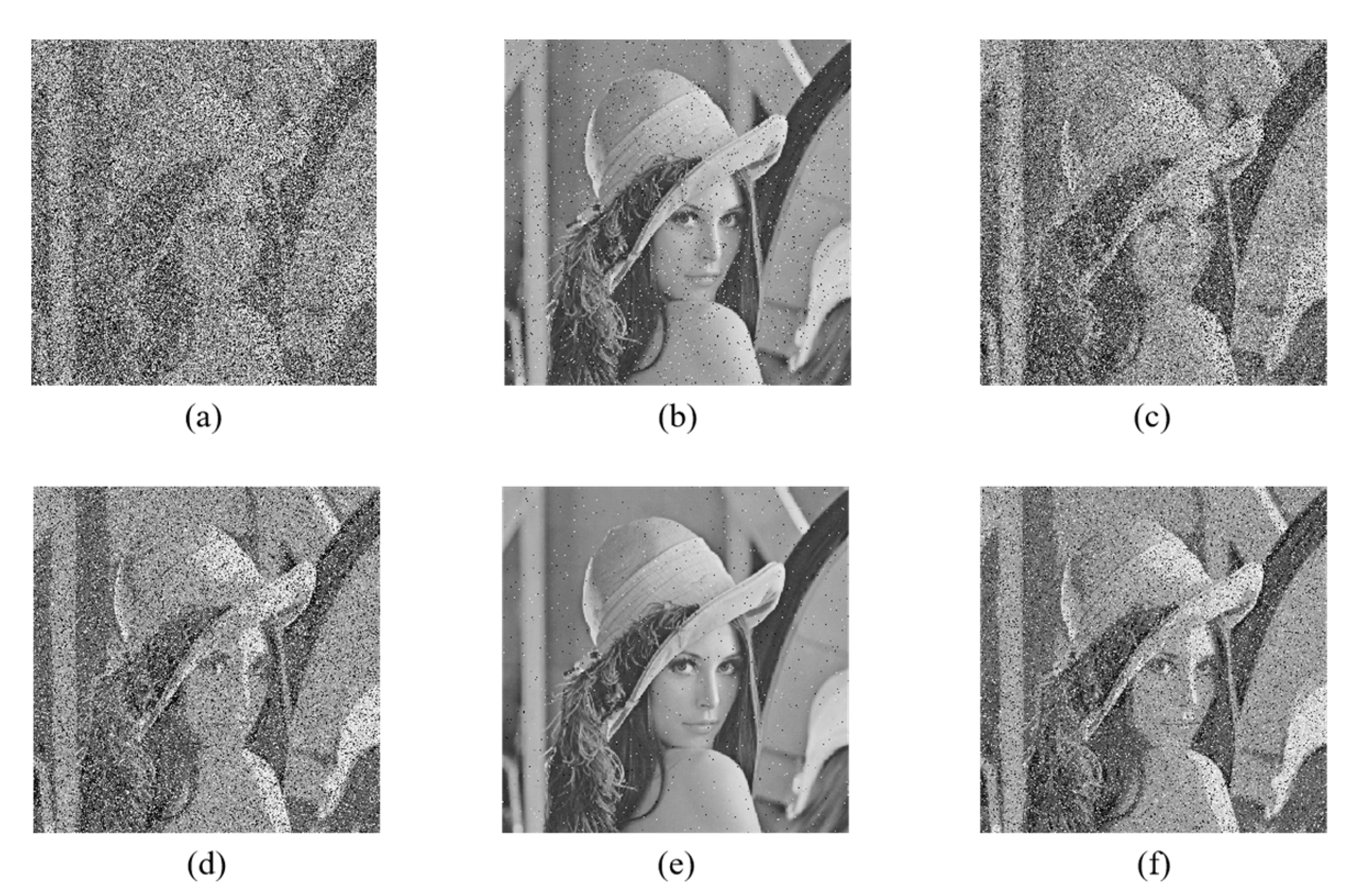
4.2.8. Noise Attack
4.3. Application in Different Size Images
4.4. Application in Color Images
5. Discussion
6. Conclusions
Author Contributions
Funding
Data Availability Statement
Acknowledgments
Conflicts of Interest
References
- Wang, X.; Yang, J. A privacy image encryption algorithm based on piecewise coupled map lattice with multi dynamic coupling coefficient. Inf. Sci. 2021, 569, 217–240. [Google Scholar] [CrossRef]
- Zhou, X.; Ma, Y.; Zhang, Q. A reversible watermarking system for medical color images: Balancing capacity, imperceptibility, and robustness. Electronics 2021, 10, 1024. [Google Scholar] [CrossRef]
- Ran, B.; Zhang, T.; Wang, L. Image Security Based on Three-Dimensional Chaotic System and Random Dynamic Selection. Entropy 2022, 24, 958. [Google Scholar] [CrossRef]
- Huang, Z.J.; Cheng, S.; Gong, L.H. Nonlinear optical multi-image encryption scheme with two-dimensional linear canonical transform. Opt. Lasers Eng. 2020, 124, 105821. [Google Scholar] [CrossRef]
- Chai, X.; Zhi, X.; Gan, Z. Combining improved genetic algorithm and matrix semi-tensor product (STP) in color image encryption. Signal Process. 2021, 183, 108041. [Google Scholar] [CrossRef]
- Kaur, M.; Kumar, V. A comprehensive review on image encryption techniques. Arch. Comput. Methods Eng. 2020, 27, 15–43. [Google Scholar] [CrossRef]
- Zhang, X.; Hu, Y. Multiple-image encryption algorithm based on the 3D scrambling model and dynamic DNA coding. Opt. Laser Technol. 2021, 141, 107073. [Google Scholar] [CrossRef]
- Liu, S.; Zhuang, Y.; Huang, L. Exploiting LSB Self-quantization for Plaintext-related Image Encryption in the Zero-trust Cloud. J. Inf. Secur. Appl. 2022, 66, 103138. [Google Scholar] [CrossRef]
- Hua, Z.; Zhu, Z.; Chen, Y. Color image encryption using orthogonal Latin squares and a new 2D chaotic system. Nonlinear Dyn. 2021, 104, 4505–4522. [Google Scholar] [CrossRef]
- Wang, X.; Gao, S. Image encryption algorithm based on the matrix semi-tensor product with a compound secret key produced by a Boolean network. Inf. Sci. 2020, 539, 195–214. [Google Scholar] [CrossRef]
- Ma, Y.; Li, C.; Ou, B. Cryptanalysis of an image block encryption algorithm based on chaotic maps. J. Inf. Secur. Appl. 2020, 54, 102566. [Google Scholar] [CrossRef]
- Zhu, C.; Gan, Z.; Lu, Y. An image encryption algorithm based on 3-D DNA level permutation and substitution scheme. Multimed. Tools Appl. 2020, 79, 7227–7258. [Google Scholar] [CrossRef]
- Chen, J.; Zhu, Z.; Zhang, L. Exploiting self-adaptive permutation–diffusion and DNA random encoding for secure and efficient image encryption. Signal Process. 2018, 142, 340–353. [Google Scholar] [CrossRef]
- Alghafis, A.; Firdousi, F.; Khan, M. An efficient image encryption scheme based on chaotic and Deoxyribonucleic acid sequencing. Math. Comput. Simul. 2020, 177, 441–466. [Google Scholar] [CrossRef]
- Wang, X.; Zhao, M. An image encryption algorithm based on hyperchaotic system and DNA coding. Opt. Laser Technol. 2021, 143, 107316. [Google Scholar] [CrossRef]
- Mohamed, A.G.; Korany, N.O.; El-Khamy, S.E. New DNA coded fuzzy based (DNAFZ) S-boxes: Application to robust image encryption using hyper chaotic maps. IEEE Access 2021, 9, 14284–14305. [Google Scholar] [CrossRef]
- Abbasi, A.A.; Mazinani, M.; Hosseini, R. Evolutionary-based image encryption using biomolecules and non-coupled map lattice. Opt. Laser Technol. 2021, 140, 106974. [Google Scholar] [CrossRef]
- Zeng, J.; Wang, C. A novel hyperchaotic image encryption system based on particle swarm optimization algorithm and cellular automata. Secur. Commun. Netw. 2021, 2021, 6675565. [Google Scholar] [CrossRef]
- Toktas, A.; Erkan, U.; Ustun, D. An image encryption scheme based on an optimal chaotic map derived by multi-objective optimization using ABC algorithm. Nonlinear Dyn. 2021, 105, 1885–1909. [Google Scholar] [CrossRef]
- Wang, X.; Liu, C.; Xu, D. Image encryption scheme using chaos and simulated annealing algorithm. Nonlinear Dyn. 2016, 84, 1417–1429. [Google Scholar] [CrossRef]
- Kaur, M.; Singh, D. Multiobjective evolutionary optimization techniques based hyperchaotic map and their applications in image encryption. Multidimens. Syst. Signal Process. 2021, 32, 281–301. [Google Scholar] [CrossRef]
- Selvi, C.T.; Amudha, J.; Sudhakar, R. A modified salp swarm algorithm (SSA) combined with a chaotic coupled map lattices (CML) approach for the secured encryption and compression of medical images during data transmission. Biomed. Signal Process. Control. 2021, 66, 102465. [Google Scholar] [CrossRef]
- Tamang, J.; Nkapkop, J.D.D.; Ijaz, M.F. Dynamical properties of ion-acoustic waves in space plasma and its application to image encryption. IEEE Access 2021, 9, 18762–18782. [Google Scholar] [CrossRef]
- Long, S. A Comparative Analysis of the Application of Hashing Encryption Algorithms for MD5, SHA-1, and SHA-512. J. Phys. Conf. Series. IOP Publ. 2019, 1314, 012210. [Google Scholar] [CrossRef]
- Pak, C.; Huang, L. A new color image encryption using combination of the 1D chaotic map. Signal Process. 2017, 138, 129–137. [Google Scholar] [CrossRef]
- Wang, K.; Li, X.; Gao, L. A genetic simulated annealing algorithm for parallel partial disassembly line balancing problem. Appl. Soft Comput. 2021, 107, 107404. [Google Scholar] [CrossRef]
- Chai, X.; Zhang, J.; Gan, Z. Medical image encryption algorithm based on Latin square and memristive chaotic system. Multimed. Tools Appl. 2019, 78, 35419–35453. [Google Scholar] [CrossRef]
- Enayatifar, R.; Abdullah, A.H.; Isnin, I.F. Image encryption using a synchronous permutation-diffusion technique. Opt. Lasers Eng. 2017, 90, 146–154. [Google Scholar] [CrossRef]
- Toktas, A.; Erkan, U. 2D fully chaotic map for image encryption constructed through a quadruple-objective optimization via artificial bee colony algorithm. Neural Comput. Appl. 2022, 34, 4295–4319. [Google Scholar] [CrossRef]
- Wu, J.; Liao, X.; Yang, B. Image encryption using 2D Hénon-Sine map and DNA approach. Signal Process. 2018, 153, 11–23. [Google Scholar] [CrossRef]


| 1 | 2 | 3 | 4 | 5 | 6 | 7 | 8 | |
|---|---|---|---|---|---|---|---|---|
| A | 00 | 00 | 01 | 01 | 10 | 10 | 11 | 11 |
| T | 11 | 11 | 10 | 10 | 01 | 01 | 00 | 00 |
| C | 01 | 10 | 00 | 11 | 00 | 11 | 01 | 10 |
| G | 10 | 01 | 11 | 00 | 11 | 00 | 10 | 01 |
| +/−/XNOR/XOR | A | T | C | G |
|---|---|---|---|---|
| A | A/A/C/A | T/G/G/T | C/C/A/C | G/T/T/G |
| T | T/T/G/T | C/A/C/A | G/G/T/G | A/C/A/C |
| C | C/C/A/C | G/T/T/G | A/A/C/A | T/G/G/T |
| G | G/G/T/G | A/C/A/C | T/T/G/T | C/A/C/A |
| Image 512 × 512 | Direction |  |  |  |  |  |  |  |
|---|---|---|---|---|---|---|---|---|
| Plain image | horizontal | 0.9847 | 0.9699 | 0.9901 | 0.9804 | 0.9122 | NaN | NaN |
| vertical | 0.9709 | 0.9726 | 0.9832 | 0.9801 | 0.9336 | NaN | NaN | |
| diagonal | 0.9586 | 0.9490 | 0.9733 | 0.9706 | 0.8666 | NaN | NaN | |
| Proposed | horizontal | −0.0002 | −0.0028 | −0.0027 | 0.0014 | 0.0029 | 0.0026 | 0.0016 |
| vertical | −0.0011 | 0.0002 | −0.0013 | 0.0012 | 0.0014 | 0.0016 | −0.0015 | |
| diagonal | 0.0015 | −0.0016 | −0.007 | 0.0011 | −0.0006 | 0.0009 | −0.0029 |
| Image 512 × 512 |  |  |  |  |  |
|---|---|---|---|---|---|
| Plaintext image | 242,173.67 | 708,178.59 | 418,530.14 | 549,151.28 | 211,365.83 |
| Encrypted image | 189.71 | 195.96 | 183.10 | 202.42 | 185.37 |
| [3] | 255.8 | 265.1 | 259.9 | 250.32 | 252.3 |
| [19] | 239.66 | 233.57 | 232.85 | 231.69 | 238.65 |
| [29] | 236.66 | 238.30 | 241.87 | 238.90 | 237.86 |
| Image 512 × 512 |  |  |  |  |  |  |  |
|---|---|---|---|---|---|---|---|
| Plain | 7.2185 | 6.7132 | 7.0480 | 6.7624 | 7.2925 | 0 | 0 |
| Proposed | 7.9995 | 7.9995 | 7.9995 | 7.9995 | 7.9995 | 7.9995 | 7.9994 |
| Image 512 × 512 |  |  |  |  |  | Average Value |
|---|---|---|---|---|---|---|
| Proposed | 7.9995 | 7.9995 | 7.9995 | 7.9995 | 7.9995 | 7.9995 |
| [3] | 7.9992 | 7.9993 | 7.9993 | 7.9993 | 7.9993 | 7.9993 |
| [17] | 7.9995 | 7.9995 | 7.9994 | 7.9994 | 7.9994 | 7.9994 |
| [19] | 7.9994 | 7.9994 | 7.9994 | 7.9994 | 7.9994 | 7.9994 |
| [28] | 7.9994 | 7.9991 | 7.9972 | 7.9983 | 7.9981 | 7.9984 |
| [30] | 7.9994 | 7.9992 | 7.9993 | 7.9993 | 7.9992 | 7.9993 |
| Image 512 × 512 |  |  |  |  |  | |
|---|---|---|---|---|---|---|
| Proposed | NPCR(%) | 99.5956 | 99.6212 | 99.6231 | 99.6056 | 99.6220 |
| UACI(%) | 33.4762 | 33.4229 | 33.4556 | 33.4904 | 33.4436 | |
| [17] | NPCR(%) | 99.5998 | 99.6245 | 99.6071 | 99.5983 | 99.6101 |
| UACI(%) | 33.4715 | 33.4506 | 33.4647 | 33.4823 | 33.4238 | |
| [28] | NPCR(%) | 99.6304 | 99.4883 | 99.2052 | 99.3017 | 99.2394 |
| UACI(%) | 33.5989 | 33.3562 | 33.4390 | 33.0026 | 33.3144 | |
| [30] | NPCR(%) | 99.6002 | 99.6261 | 99.6082 | 99.6112 | 99.5903 |
| UACI(%) | 33.5079 | 33.5782 | 33.5574 | 33.5265 | 33.5281 |
| Cropping Degree | 25% | 50% | 75% | |
|---|---|---|---|---|
| NPCR(%) | [3] | 24.9126 | 49.8211 | 74.7200 |
| Proposed | 25.0576 | 49.9805 | 74.8482 |
| Image 256 × 256 |  |  |  | |
|---|---|---|---|---|
| Information entropy | 7.9976 | 7.9974 | 7.9976 | |
| correlation coefficient | horizontal | 0.0046 | −0.0009 | 0.0015 |
| vertical | −0.0012 | 0.0039 | −0.0011 | |
| diagonal | 0.0015 | −0.0043 | −0.0041 | |
| 216.5391 | 239.7344 | 212.9531 |
 |  |  |  | |
|---|---|---|---|---|
| Information entropy | 7.9994 | 7.9994 | 7.9994 | |
| correlation coefficient | horizontal | 0.0025 | −0.0033 | 0.0015 |
| vertical | 0.0014 | 0.0012 | −0.0011 | |
| diagonal | −0.0022 | 0.0014 | −0.0041 | |
| 211.1387 | 207.0215 | 201.7012 |
Disclaimer/Publisher’s Note: The statements, opinions and data contained in all publications are solely those of the individual author(s) and contributor(s) and not of MDPI and/or the editor(s). MDPI and/or the editor(s) disclaim responsibility for any injury to people or property resulting from any ideas, methods, instructions or products referred to in the content. |
© 2023 by the authors. Licensee MDPI, Basel, Switzerland. This article is an open access article distributed under the terms and conditions of the Creative Commons Attribution (CC BY) license (https://creativecommons.org/licenses/by/4.0/).
Share and Cite
Zhang, T.; Zhu, B.; Ma, Y.; Zhou, X. A Novel Image Encryption Algorithm Based on Multiple Random DNA Coding and Annealing. Electronics 2023, 12, 501. https://doi.org/10.3390/electronics12030501
Zhang T, Zhu B, Ma Y, Zhou X. A Novel Image Encryption Algorithm Based on Multiple Random DNA Coding and Annealing. Electronics. 2023; 12(3):501. https://doi.org/10.3390/electronics12030501
Chicago/Turabian StyleZhang, Tianshuo, Bingbing Zhu, Yiqun Ma, and Xiaoyi Zhou. 2023. "A Novel Image Encryption Algorithm Based on Multiple Random DNA Coding and Annealing" Electronics 12, no. 3: 501. https://doi.org/10.3390/electronics12030501