Abstract
A laser beam propagating in the free space suffers numerous degradation effects. In the context of free space optical communications (FSOCs), this results in reduced availability of the link. This study provides a comprehensive comparison between six machine learning (ML) regression algorithms for modeling the refractive index structure parameter (. A single neural network (ANN), a random forest (RF), a decision tree (DT), a gradient boosting regressor (GBR), a k-nearest neighbors (KNN) and a deep neural network (DNN) model are applied to estimate from experimentally measured macroscopic meteorological parameters obtained from several devices installed at the Naval Postgraduate School (NPS) campus over a period of 11 months. The data set was divided into four quarters and the performance of each algorithm in every quarter was determined based on the R2 and the RMSE metric. The corresponding RMSE were 0.091 for ANN, 0.064 for RF, 0.075 for GBR, 0.073 for KNN, 0.083 for DT and 0.085 for DNN. The second part of the study investigated the influence of atmospheric turbulence in the availability of a notional FSOC link, by calculating the outage probability (Pout) assuming a gamma gamma (GG) modeled turbulent channel. A threshold value of 99% availability was assumed for the link to be functional. A DNN classification algorithm was then developed to model the link status (On-Off) based on the previously mentioned meteorological parameters.
1. Introduction
The free space optical communications (FSOCs) technology has drawn the attention for quite a few decades since its inherent advantages cannot be neglected. Compared to radio frequency technology, FSOCs offer higher data rate, are easier and lower cost to install, provide more immunity and security, and have less license restrictions [1]. Already, laser data rates of 10 Gbps have been demonstrated in the field for both air-to-ground and air-to-air long range FSO links, whereas for shorter ranges they have reached 100 Gbps [1]. However, the use of a laser beam propagating through the atmosphere results in several challenges that need to be overcome in order to avoid performance degradation of the FSO link. Atmospheric attenuation in the form of scattering and absorption tends to decrease the available power to the receiver, whereas optical turbulence causes scintillation, beam spreading and beam wandering [1]. The inability of an FSO link to operate in any weather condition and range has also promoted the hybridization of the communications scheme to include both radio frequency and laser operational modes. The criterion for the mode selection is the availability of the lasercomm link. Once it is non-operable, these systems should automatically switch to the radio frequency mode. Therefore, it is of significant interest to predict the availability of the link based upon the current atmospheric conditions.
The purpose of this paper is two-fold. First, to introduce the application of machine learning algorithms in modeling the refractive index structure parameter and estimate its value through regression analysis of macroscopic meteorological parameters. Second, to apply well known mathematical expressions to estimate the outage probability of a notional FSO link based on the strength of the optical turbulence and to model the link status (On-Off) based on macroscopic meteorological parameters by utilizing a DNN classification algorithm. Various experimental research papers exist in the literature on the topic of optical turbulence prediction and FSO performance modeling [2]. Lionis et. al. modeled the received signal strength indicator (RSSI) parameter of a FSO link over a maritime environment based on meteorological parameters. The comparison with different theoretical models presented good agreement [3,4,5]. Jellen et. al. in their work established a scintillometer link along Chesapeake Bay and showed that existing predictive models for , developed for an open ocean environment, performed poorly in a near-maritime environment [6]. Such models were developed by Wang et. al. based on micrometeorology, macrometeorology and the Monin-Obukhov similarity (MOS) theory; none of these models performed best across all atmospheric conditions (i.e., overcast sky, sunny day, cloudy day) [7]. Basu, proposed a physically-based approach to estimate utilizing the Thorpe scale for outer scale turbulence measurement which requires only coarse resolution temperature profiles as input and provides layers of high optical turbulence [8]. An urban area FSO link is developed in [9] coupled with optical/meteorological measurements. The performance of the link under turbulence, precipitation, dust and flying objects is studied with a focus on water particles effects. Rafalimanana et al. used a numerical approach by weather and research forecasting (WRF) modeling coupled with different turbulence models in order to forecast the vertical profiles of meteorological parameters and [10]. Finally, alternative FSO geometries studied to include satellite laser communications [11] and drone-to-ground FSO links [12].
Over the last decade, application of ML techniques has constantly gained higher interest among the FSOC community. Modeling the extremely nonlinear atmospheric phenomena with traditional methods, while acceptable, still requires significant improvement. Several attempts at using ML to improve upon these traditional techniques can be found in literature. Mishra et. al. established an FSO link through an optical turbulence generating (OTG) chamber to estimate the channel coefficients using Maximum Likelihood (MLE) and Bayesian techniques and to show that for certain power levels, increasing the pilot symbol length resulted in lower bit error rate (BER) [13]. Vorontsov et. al. compared the results of experimental data with wave-optics numerical simulation data and developed a DNN model that was verified against other ML algorithms with good accuracy and high temporal resolution [14]. Lohani et. al. developed a state-of-the-art combined Generative and Convolutional Neural network system and demonstrated its efficacy in both experimental and simulated communication settings. Their system demonstrated a reduction in the detector noise and correction of distortion [15]. In [16], Lamprecht et. al. proposed a residual network (ResNet) approach for estimation without location dependence as most mathematical models have. An artificial neural network (ANN) was used by Wang and Basu to predict from routine meteorological parameters measurements near the land surface, and verified the capacity of such an approach to model highly complex data sets [17]. A long range propagating laser beam can result in blurred and distorted visual images which requires highly efficient mitigation methods to compensate those aberrations. To that end, extended research using deep learning algorithms has been applied to mitigate turbulence effects [18,19]. However, the literature review reveals that many of the ML algorithms have not yet been applied in the area of FSOs [20]; therefore, this paper aims to add more insights towards this direction. In a previous work, we have demonstrated the accuracy of various ML algorithms towards the performance prediction of an FSO link over maritime environment, by modeling the received signal strength indicator (RSSI) [21]. This paper is focused again on the performance of such a link but this time the focus is on applying ML algorithms to model and outage probability (Pout). The rest of the paper is organized as follows: Section 2 provides the theoretical background of optical turbulence and its effects on a laser beam as well as the mathematical background for channel modeling and performance metrics. Section 3 describes the setup used to collect the data at the NPS campus. Section 4 presents a thorough data analysis as well as the results of the various ML algorithms for both for and Pout prediction. Section 5 provides the discussion on the results and the conclusion of the paper.
2. Atmospheric Optical Turbulence
Small variations of temperature in the atmosphere result in changes of the refractive index that can disturb the phase and intensity profiles of an optical wave. Optical turbulence in the form of these eddies of differing refractive indices is difficult to model from first principles; instead, these refractive index changes are usually described using a statistical approach [22].
Kolmogorov was one of the first to examine in depth the phenomenon of optical turbulence by simplifying the complex Navier-Stokes equations that describe it. He defined two distinct flow states for a viscous fluid: laminar flow (with uniform streamlines) and turbulent (with chaotic streamlines). The dimensionless Reynolds number can be used to distinguish between these two regimes [22]. Assuming the flow is turbulent, then Richardson energy cascade theory is used to describe the transfer of energy from the largest characteristic eddy size L0 to the smallest eddy size l0 (where the energy is dissipated as heat). Eddies between these two sizes fall within the so-called inertial subrange.
The index of refraction is closely related to temperature and pressure variations [22],
where P is the pressure in millibars and T is the temperature in kelvin. Under the assumptions of statistical homogeneity and isotropy, the structure function of the refractive index for the inertial subrange is [22]
where the refractive index structure parameter in units of m−2/3. Larger values of this parameter correlate to stronger optical turbulence; i.e., characterizes the strength of the fluctuations of the refractive index. The value of varies significantly both spatially and temporarily; however, it can be estimated at a certain point in space using the difference of temperatures between two locations separated by a distance . Specifically, we can extract the temperature structure constant [22],
which is related with the by [22].
An extended number of empirical models for prediction exists, varying in the type of terrain they are applicable to, their effective range and the kind and sensitivity to the inputs they require. A comprehensive list with such models can be found in Table 2.5 [23].
2.1. Channel Modeling
The fluctuations of the irradiance at the receiver of a terrestrial FSO system caused by the propagation through atmospheric turbulence result in a phenomenon called “scintillation”. It can lead to significant power losses and eventually communication disruption. The measurement of scintillation index (S.I.) is achieved through the normalized value of irradiance in the receiver defined as [24],
where the ensemble average of the squared irradiance values. The log irradiance (a.k.a Rytov variance) is related to S.I. as below [22],
Turbulence strength can be classified in the weak, moderate, and strong regimes. In the weak regime for a plane wave, and coincide [22],
and for a spherical wave [22],
where is the wavenumber. Equations (7) and (8) for the strong turbulence regime convert as following [22],
and
From Equations (9) and (10) it is seen that shorter wavelengths experience smaller irradiance fluctuations. It is of significant importance to be able to model those fluctuations. For that reason, many studies have been devoted to develop the probability density function (PDF) of the irradiance fluctuations at the receiver for every turbulence strength regime. The result of these studies is the existence of a large set of PDFs, each with a different degree of accuracy. Most of these models are applicable to a certain turbulence strength regime but have a very low accuracy in a different one. For example, the well-known lognormal model describes only the fluctuations in the weak regime. This paper utilizes experimentally derived data, with values spanning over every regime; therefore, we apply the gamma gamma (GG) distribution which is more suitable in our case and can also be expressed in closed form. Irradiance fluctuations in GG model are represented by two independent variables, Ix and Iy, which refer to the large and small scale turbulent eddies, respectively and follow the gamma distribution. The PDF of this distribution is given [24],
where is the modified Bessel function of second kind of order α. A great advantage of this distribution is that it directly relates the irradiance fluctuations with the atmospheric conditions and certain design characteristics through the parameters α and β (i.e., the effective number of small and large-scale eddies) given by the following expressions [24],
and
where , L the distance between the transmitter and receiver of an FSO system, and D the aperture diameter of the receiver. The scintillation index can also be expressed in terms of those two parameters as follows [24],
By employing [25], Equations (1.12.1/2), the corresponding cumulative distribution function (CDF) can be deduced in closed-form as,
where ξ = αβ and is the generalized hypergeometric function.
2.2. Performance Metrics
As described in the previous paragraphs, the atmospheric turbulence causes fading of the signal from a propagating laser beam, which within the context of laser communications affects the reliability of an FSO link. The optical turbulence effects on the beam include the intensity decrease of the received signal; below a threshold value it can even cause outage of the link. The frequency of the signal intensity fluctuations, as compared to the bit rate of the channel, characterizes the fading statistics that describe this channel. Fast fading statistics refer to the case where the fluctuations are much more rapid than the bit rate, whereas slow statistics refer to the case where these fluctuations are slow as compared to the bit rate. A performance metric that is useful for both fast and slow fading statistics is the outage probability (Pout) of the link [24]. Pout is defined as the probability that the instantaneous SNR in the receiver falls below a critical threshold that is determined by the sensitivity of the receiver. Apparently, the lower this probability the more reliable the FSO link. The relationship between the irradiance and the SNR on the receiver is given by the expression [24],
where γ and μ are the instantaneous and the average electrical SNR, respectively. Substituting Equation (16) in Equation (11) and with a power transformation of I, we obtain the PDF of the irradiance in terms of the instantaneous SNR on the receiver [24],
Therefore, as stated before, if we assume γth to be the threshold value of the instantaneous SNR in the receiver, we define the outage probability for a channel modeled with the GG distribution as follows [24],
3. Experimental Setup
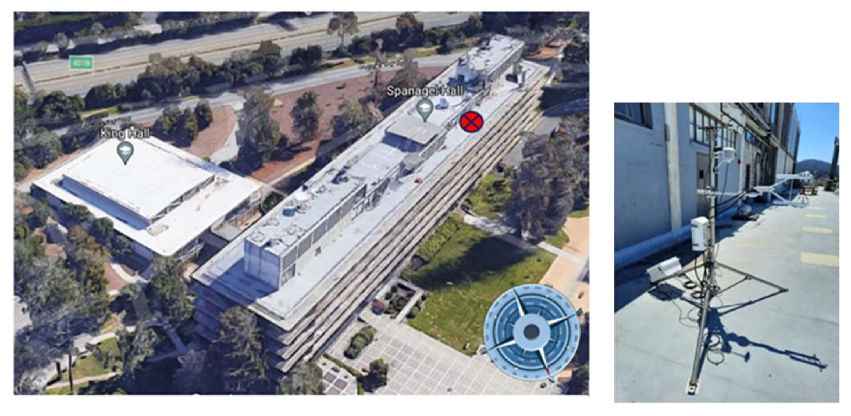
The whole experimental setup has been installed on the roof of Spanagel Hall at the Naval Postgraduate School, at an elevation of about 20 m above sea level and was a follow up to the Monterey bay experimental campaign presented in [26]. Figure 1 depicts the experimental apparatus, consisted of a tripod with four instruments: an IRGASON (Integrated CO2/H2O Open-Path Gas Analyzer and 3D Sonic Anemometer), an Apogee infrared radiometer, an Apogee SN500SS net radiometer, and a Garmin global positioning system (GPS) receiver [27]. The entire system was oriented to the northwest (facing Monterey Bay). This allowed the bay’s onshore winds to flow across the device, while the building prevented southeasterly winds. From late January till late November 2021, continuous data collection was conducted. The obtained data included air temperature, ground (roof) temperature, solar flux, wind speed, sonic temperature and water vapor concentration readings.

Figure 1.
The experimental setup location on the roof of Spanagel Hall (left) and the instruments utilized to obtain the macroscopic meteorological parameters (right).
The IRGASON is a three-dimensional sonic anemometer with an integrated optical gas analyzer. The estimates of turbulence were calculated from the sonic temperature and wind speed data provided by this instrument. The infrared radiometer is a sensor used to detect surface temperature by monitoring the surface’s blackbody radiation. Part of the shortwave light (between 280 and 4000 nm) emitted by the sun is reflected by the Earth’s surface. Atmospheric and terrestrial molecules absorb solar radiation and emit it as longwave thermal radiation (between 4 and 100 mm). Net radiation flux is the difference between inbound (downwelling) and outgoing (upwelling) radiation. Differences between incoming and outgoing shortwave radiation provide information regarding the amount of solar radiation absorbed by the ground. Consequently, the SN500SS net radiometer was utilized to compute the solar flux. Finally, the GPS receiver GPS16X-HVS served as a clock for this experiment, since the datalogger’s clock was set to synchronize with the GPS data automatically.
The values were extracted from the sonic anemometer based upon the Kolmogorov’s mathematical expression that relates, within the inertial subrange, the amplitude and frequency of the sonic temperature fluctuations as follows,
which results in a −5/3 slope on a log-log plot of the PSD against frequency. Therefore, fitting a line on PSD gives us the and from Equation (4) we get . The ML algorithms were then trained on the logarithm (base 10) of those estimated values.
4. Results
The data collected from the instruments presented on the previous section included air temperature (T), wind speed (UmSonic), water vapor concentration (H2O), solar flux (SF), air pressure (Pair) and ground temperature (IRtemp) as independent macroscopic meteorological parameters. As also described previously, we utilized Kolmogorov theory to extract the refractive index structure parameter from the sonic temperature and wind speed obtained from the IRGASON, which used as the dependent variable for our modeling purposes. An almost 40 second interval power spectral density (PSD) of the sonic temperature (i.e 2048 observations at a 50 Hz frequency) provided the . Average values for all other measurements were calculated over the same time interval. That gave us almost 525,000 observations of , in addition to the routine meteorological parameters, which were stored for further analysis. The complete dataset can be found in [28].
4.1. Data Analysis
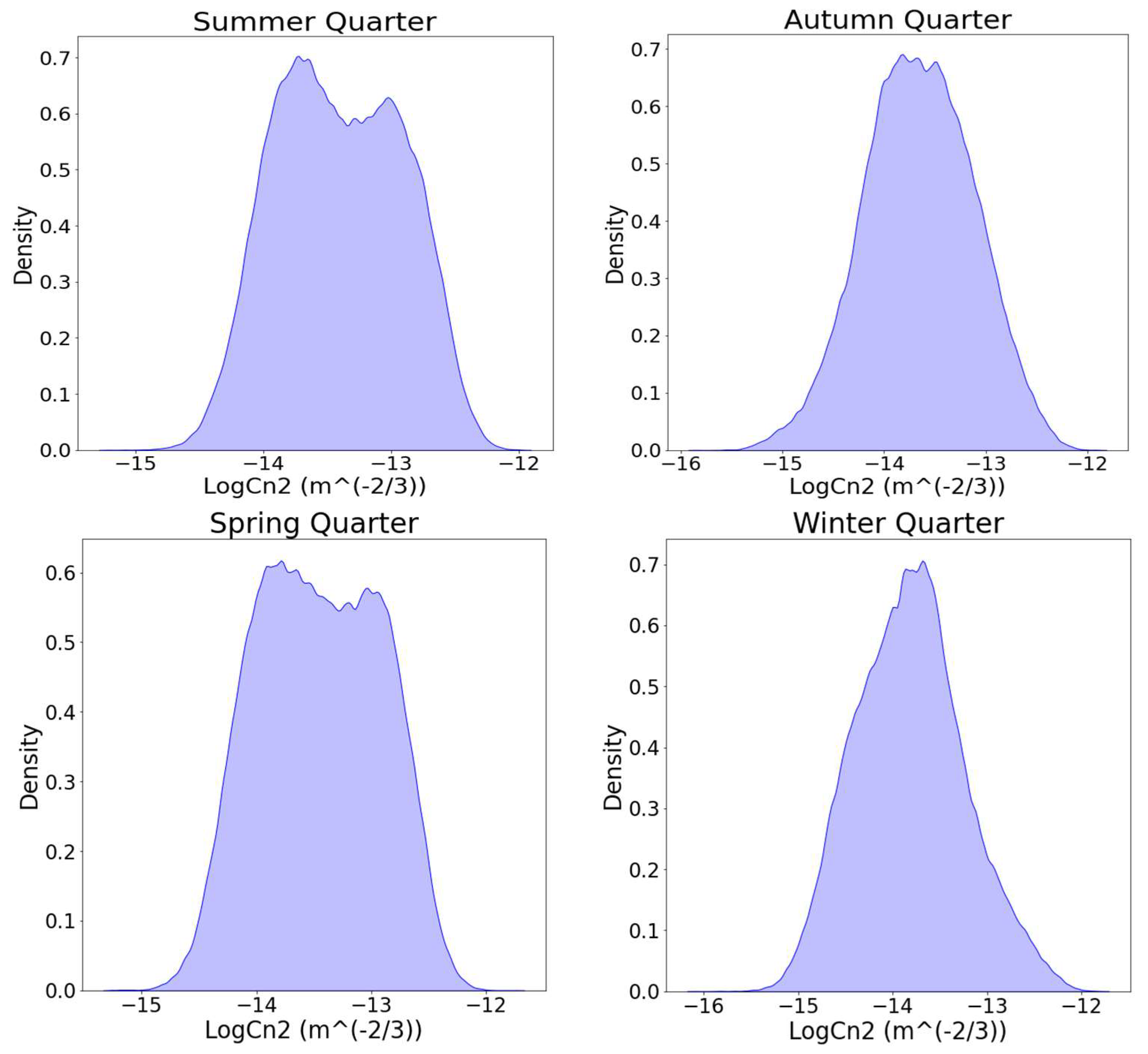
The data obtained spanned a period of almost eleven months. That means that the meteorological parameters, primarily the temperatures, had a significant variance due to their seasonal dependence. To include this seasonal dependence on our analysis, as well as to have a more effective manipulation of the datasets, we divided the whole dataset in four distinct sets of almost equal size. These different sets represent, but not precisely coincide with, the four seasons. However, since they are almost a match to the four seasons, we treated each one of them as a season representative (i.e., autumn (1 September–20 October), winter (25 January–31 March), spring (1 April–30 June) and summer (1 July–31 August)), as shown in Datasets 1 through 4 [28]. This was done primarily to observe any seasonal effect on the . Table 1 summarizes the descriptive statistics of over each season as well as the corresponding statistics for the entire experimental period. Figure 2 also presents the distribution plot of , in a logarithmic scale, for every season. Apparently, the refractive index parameter is a very complex metric to extract definite conclusions, since multiple non-linear phenomena affect its value; however, an approximate analysis can be done. To that end, Figure 3 shows the daily moving average for the entire period of every season. We notice that during winter, exhibits, in average, the lower values in contrary with summer where we observe the higher values. This is partially supported by the fact that the mean observed value of in winter is the lowest, whereas in summer is the highest. It is interesting though to mention that during winter we observed a higher maximum value for than in summer. During spring and autumn, the corresponding mean values reside within the rest two. In general, the time series of all seasons, follow the same pattern. Another characteristic of values is that during winter and autumn we observed much lower variances as compared to summer and spring (Figure 2).

Table 1.
Descriptive Statistics for .
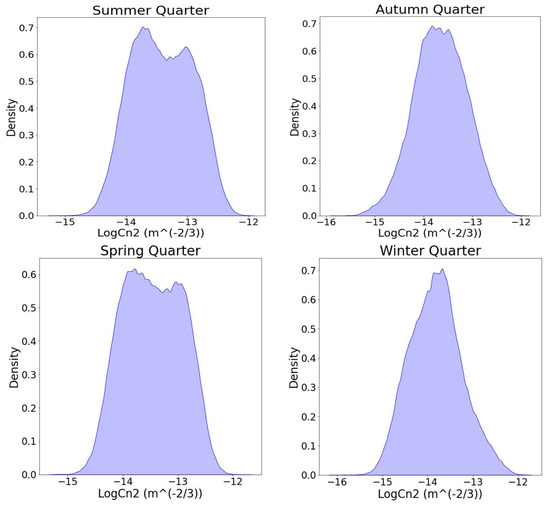
Figure 2.
Distribution plots for per season.
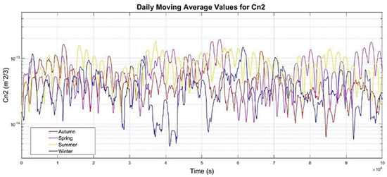
Figure 3.
The daily moving average of the for every season.
Finally, the correlation between the measured atmospheric parameters and for the entire period, is depicted in the heatmap of Figure 4. In this figure, we have included an additional parameter Dtemp, defined as the difference between the ground and the air temperature, which has a significant negative effect on . The darker a cell the stronger the anti-correlation between the corresponding two parameters. On the other hand, a lighter cell corresponds to a stronger correlation.
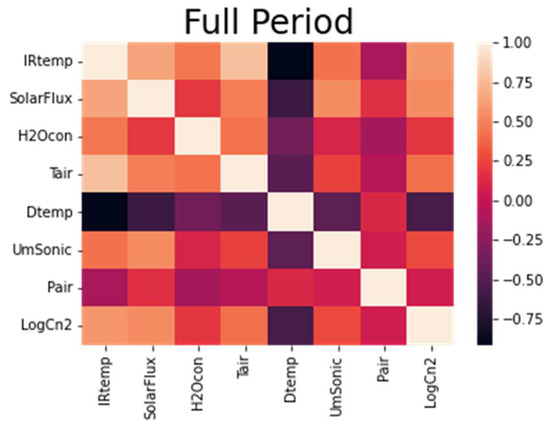
Figure 4.
Correlation matrix for the macroscopic meteorological parameters and .
4.2. Regression Analysis for Modeling
The analysis of this paper is based on the extended number of observations taken from January to November 2021. During this period, we didn’t face any technical issues, therefore our dataset can be considered continuous. Additional data cleaning before analysis, reduced the data points to a total amount of 524,786, on a ~40 second interval. The measured data obtained from all sensors, was logged into an xlsx file format, i.e., six columns. Each data row was then matched with the respective output value of for the same date/time. We excluded measurements with missing or non-physical values. That is, values above 2·10−12·m−2/3 that are not considered realistic. After collecting, compiling and cleaning the data set, the ML process was initiated. The first step was to take the set of all observations and divide it randomly into two subsets. The first subset was used to train the model. The second subset was used to test the model once it had been trained. This second dataset is referred to as the test subset. The objective was to estimate the performance of the ML model on unknown data, i.e., data not used to train the model. We chose to split at 80% for training and 20% for testing. Certain performance measures should be used in order to measure how well the models performed comparing to each other on predicting values using the test set for inputs. We applied the RMSE which represents the square root of the variance and the coefficient of determination, and R2, a number between 0 and 1 that measures how well a statistical model predicts an outcome. Lower values for RMSE and higher values for R2 are indicative of a better predictive performance. All data during the preparation phase has been scaled from 0 to 1 scale so as to account for the different variance of each parameter. The data analysis was performed using the programming language Python (version 3.8) in a Jupyter Νotebook environment, a web-based interactive computing notebook, which allows the implementation of various libraries, e.g., Pandas, Numpy, Matplotlib, Seaborn, for advanced data analytics and visualization.
To execute the regression modeling analysis, we utilized six well-known ML algorithms: Artificial Neural Networks (ANN), Random Forest (RF), Gradient Boosting Regressor (GBR), k-Nearest Neighbor (KNN), Decision Trees (DT) and Deep Neural Networks (DNN). It is out of scope of this paper to include a detailed discussion about the background of each algorithm; instead, we aim to present and compare the performance of each in modeling . As mentioned above, the same analysis was repeated for all seasons and each algorithm was fine tuned to achieve the best accuracy. The following sections present these results and comment on the selected hyperparameters for each algorithm.
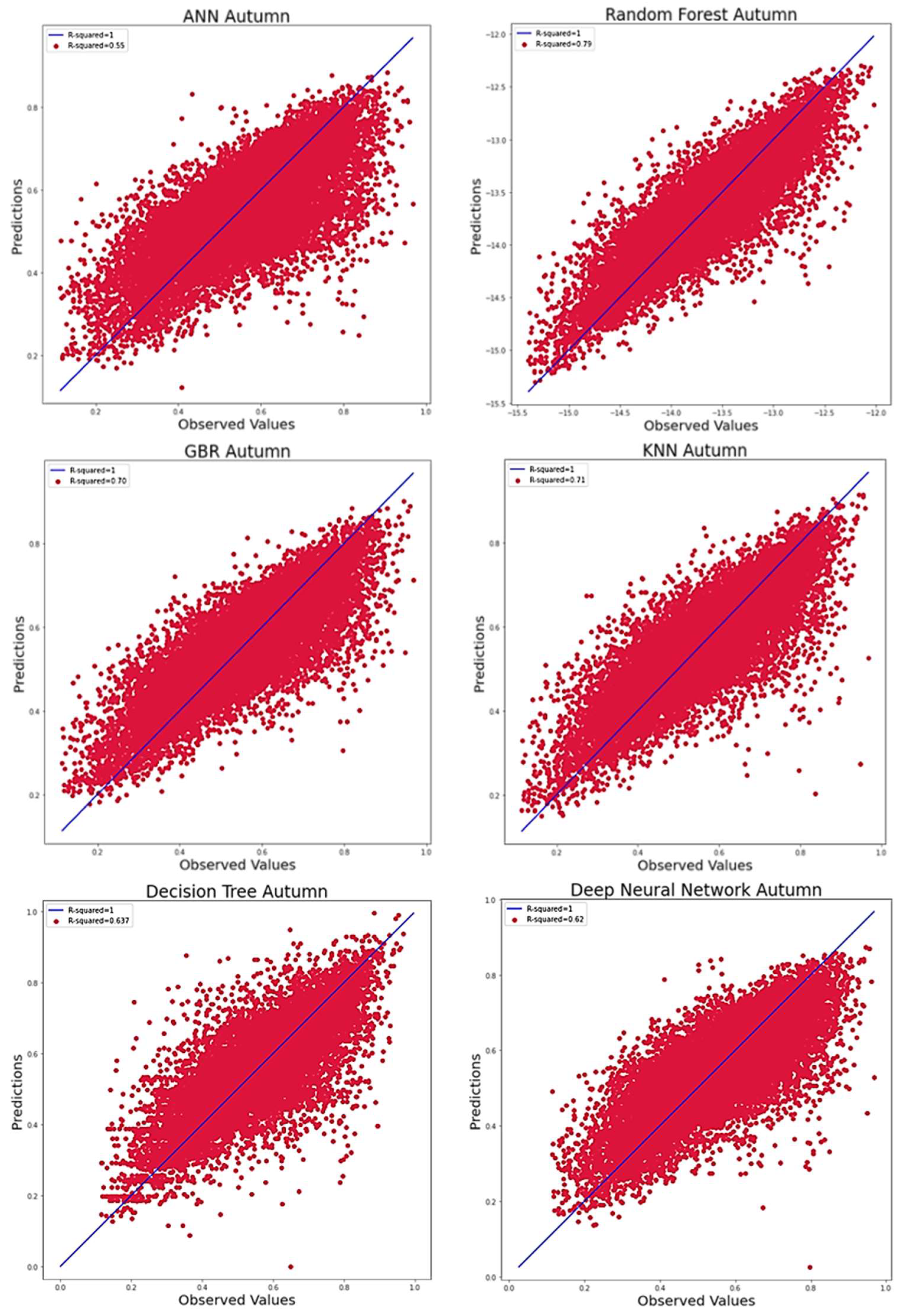
The ANN that best fitted the observed data during autumn was a single layer perceptron model that included 100 neurons in its hidden layer. The optimum batch size was 32 and the model trained over 400 epochs. A standard Levenberg-Marquardt learning method was used to train the feed-forward network with sigmoid hidden neurons and linear output neurons. The results of this algorithm showed a moderate to low accuracy, with R2 = 0.55 and RMSE = 0.0916.
The results for the RF algorithm in our data set gave a significantly improved coefficient of determination, R2, for the model evaluation of 0.78 which was the best value among all algorithms for autumn. An ensemble of 300 different trees was sufficient to construct the model with the highest possible accuracy. Additionally, an RMSE = 0.064 showed a great improvement in the error of the predicted values.
A Gradient Boosting Regressor model was used to fit the autumn data set by using a tree number -iterations- of 2000, maximum depth = 6, minimum sample split = 12 and a learning rate of 0.05. The model performed sufficiently and was comparable to the RF by achieving a value of R2 = 0.7 and an RMSE = 0.075.
The KNN algorithm achieved its best performance for a value of k = 15 which resulted in R2 = 0.71 and an RMSE = 0.073. That is, it slightly outperformed the GBR algorithm.
The DT algorithm, which is a simplified version of the RF model, as expected had poorer performance than RF. The optimum depth of trees was found to be 15 for this occasion with a corresponding R2 = 0.637 and an RMSE = 0.083.
Finally, perhaps the most complex and demanding to fine tune, DNN algorithm, comprised of three layers of neurons (1st hidden layer = 50, 2nd hidden layer = 30 and 3rd hidden layer = 10), ran over batches of 32 for a total number of 400 epochs. The results for this model were R2 = 0.61 and an RMSE = 0.085. Figure 5 collectively presents the scattering plot for each algorithm.
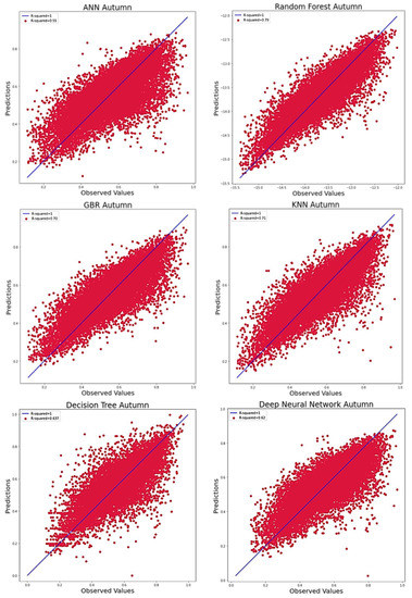
Figure 5.
Scattering plots of the six ML algorithms for the autumn data set.
The results of the performance for all ML algorithms are presented collectively in Figure 6, where the performance ranking is clearly depicted and show that the RF exhibited the best fit.
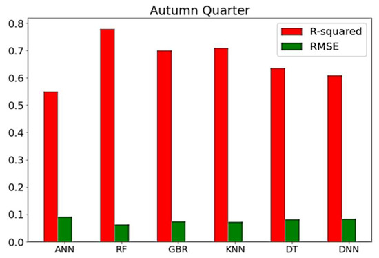
Figure 6.
R2 and RMSE metrics for the ML algorithms autumn data set.
We presented detailed results for the performance of each algorithm with regard to the autumn dataset, but the same procedure was followed repeatedly for every seasonal dataset. Therefore, we directly plot in Figure 7, Figure 8 and Figure 9 the corresponding algorithm performance metrics comparison.
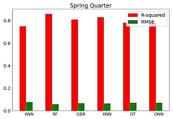
Figure 7.
R2 and RMSE metrics for the ML algorithms spring data set.

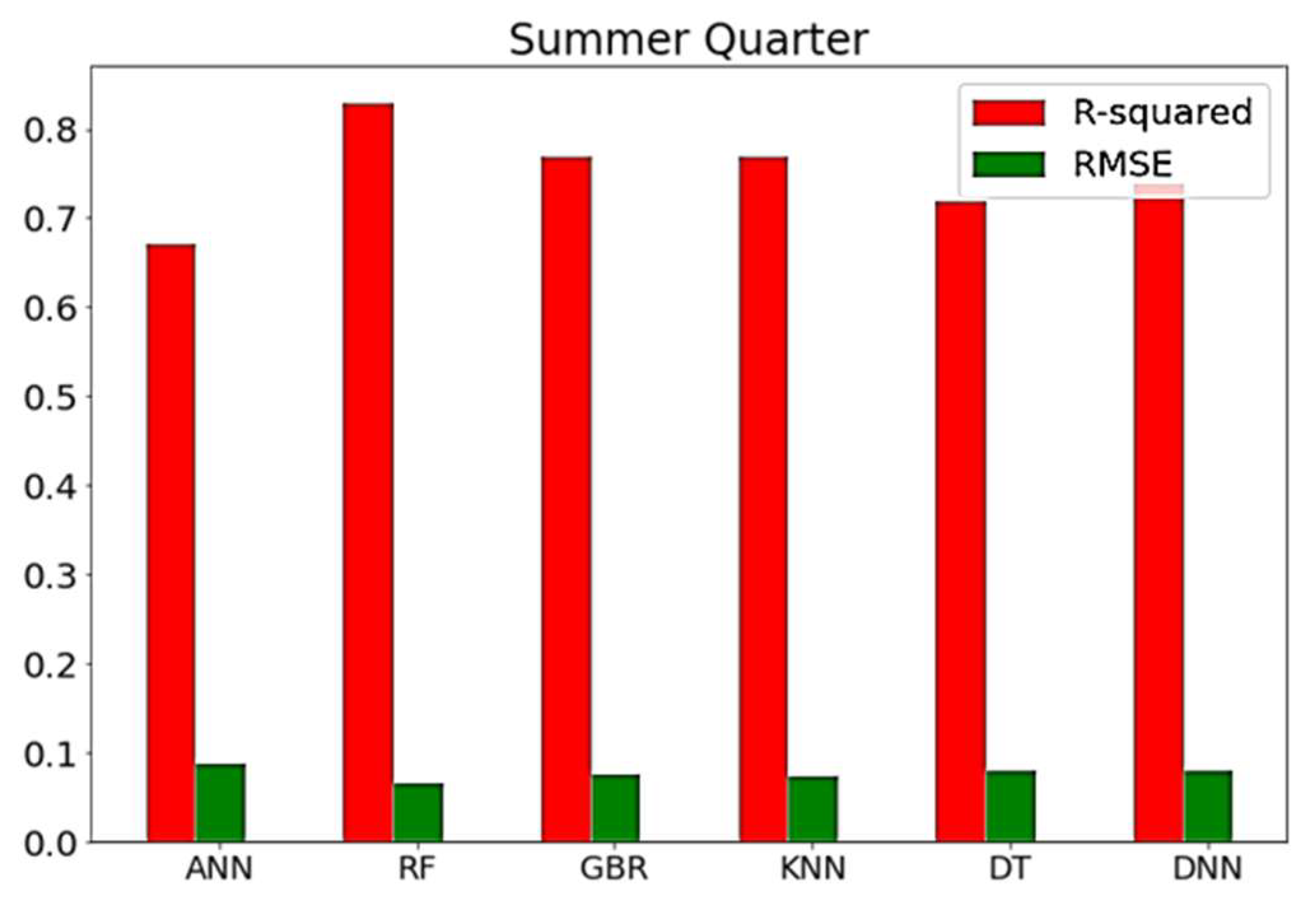
Figure 8.
R2 and RMSE metrics for the ML algorithms summer data set.

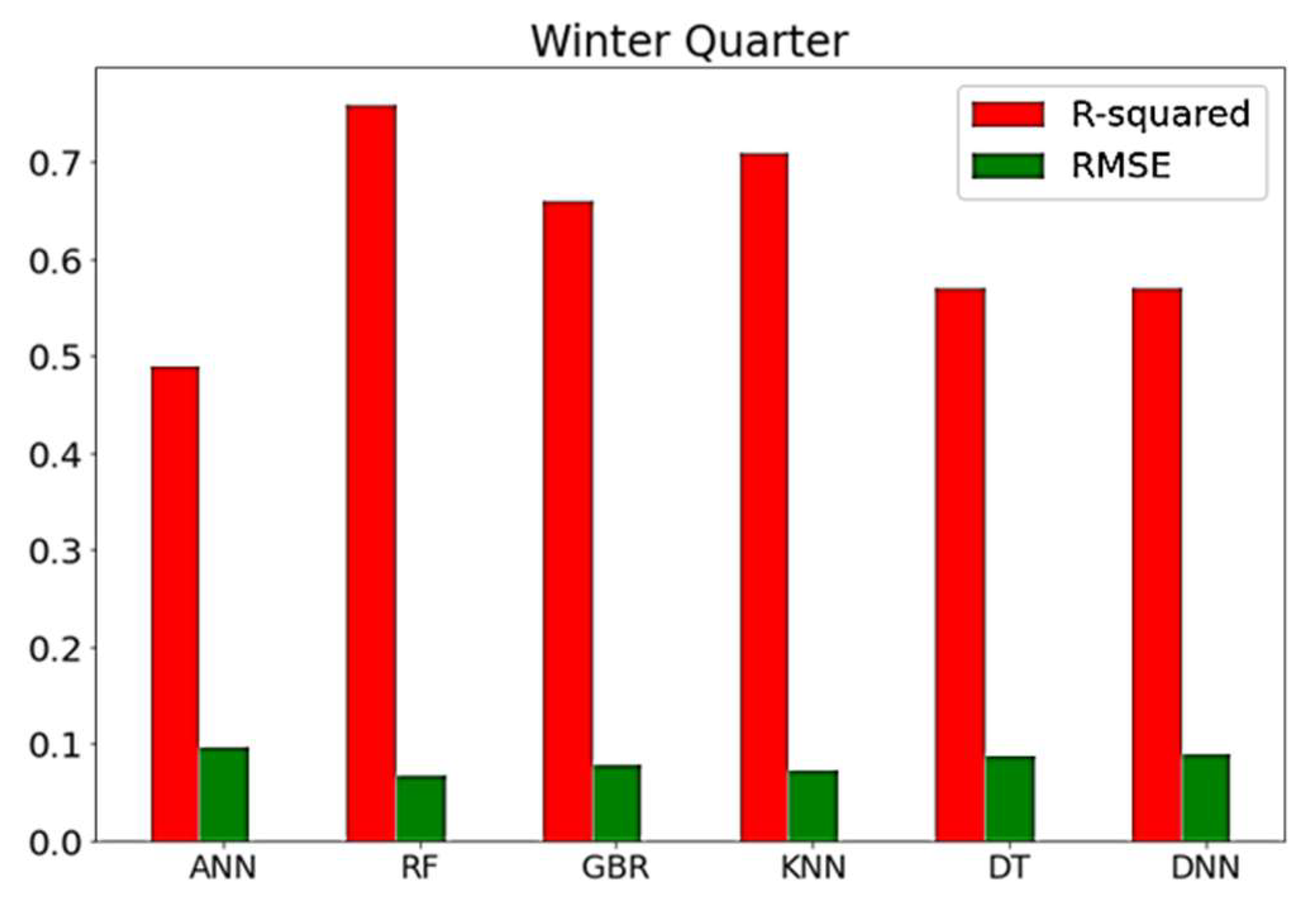
Figure 9.
R2 and RMSE metrics for the ML algorithms winter data set.
To conclude this section, it is important to comment on the overall performance of each algorithm. RF appeared to be the best, since it achieved the highest metrics values on every season. Interestingly, the next best was KNN, followed closely by GBR. DT and DNN also demonstrated similar performance to each other, but poorer than GBR. Finally, ANN had the worst fit over all datasets.
4.3. Outage Probability Calculation
The next step on our analysis was the estimation of the outage probability for a notional FSO link based on the experimental meteorological and optical turbulence data.
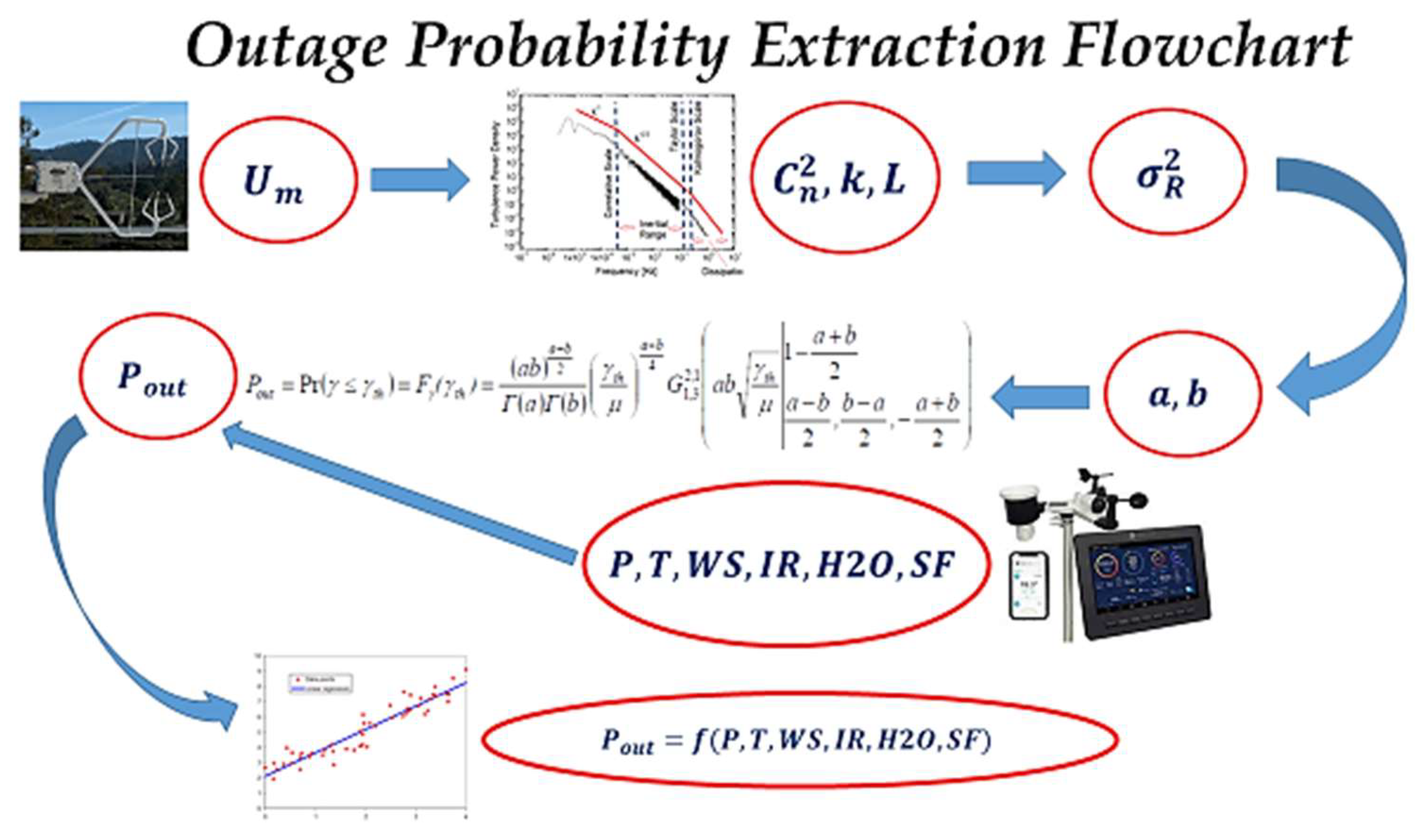
Initially, the experimental data was utilized to compute the Rytov variance, Equation (7) for a plane wave, , along with a typical wavelength λ = 850 nm and a link range, R = 3000 m. The same parameters plus , with D = 20 cm for the diameter of the FSO receiver, allowed us to calculate the environmental dependent parameters α and β from Equations (12) and (13). We assumed a typical SNR level By applying Equation (18), we were then able to compute the corresponding outage probability for every measurement instance, thus a total of almost 525,000 data points for all four seasons. The last step, described in Section 4.5, was to model the outage probability based on the six measured meteorological parameter and build a mathematical expression. A flowchart of the overall process is depicted in Figure 10. Table 2 summarizes the descriptive statistics for Pout.
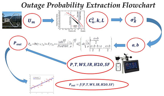
Figure 10.
The outage probability of a notional FSO link extraction flowchart. The sonic anemometer measurement allows for the extraction and consequently the Rytov variance which is used for the alpha and beta parameters. Equation (18) applies those values and calculates the outage probability which later on is modeled based on the experimentally measured atmospheric parameters.
Table 2.
Descriptive Statistics for .
4.4. DNN Classification
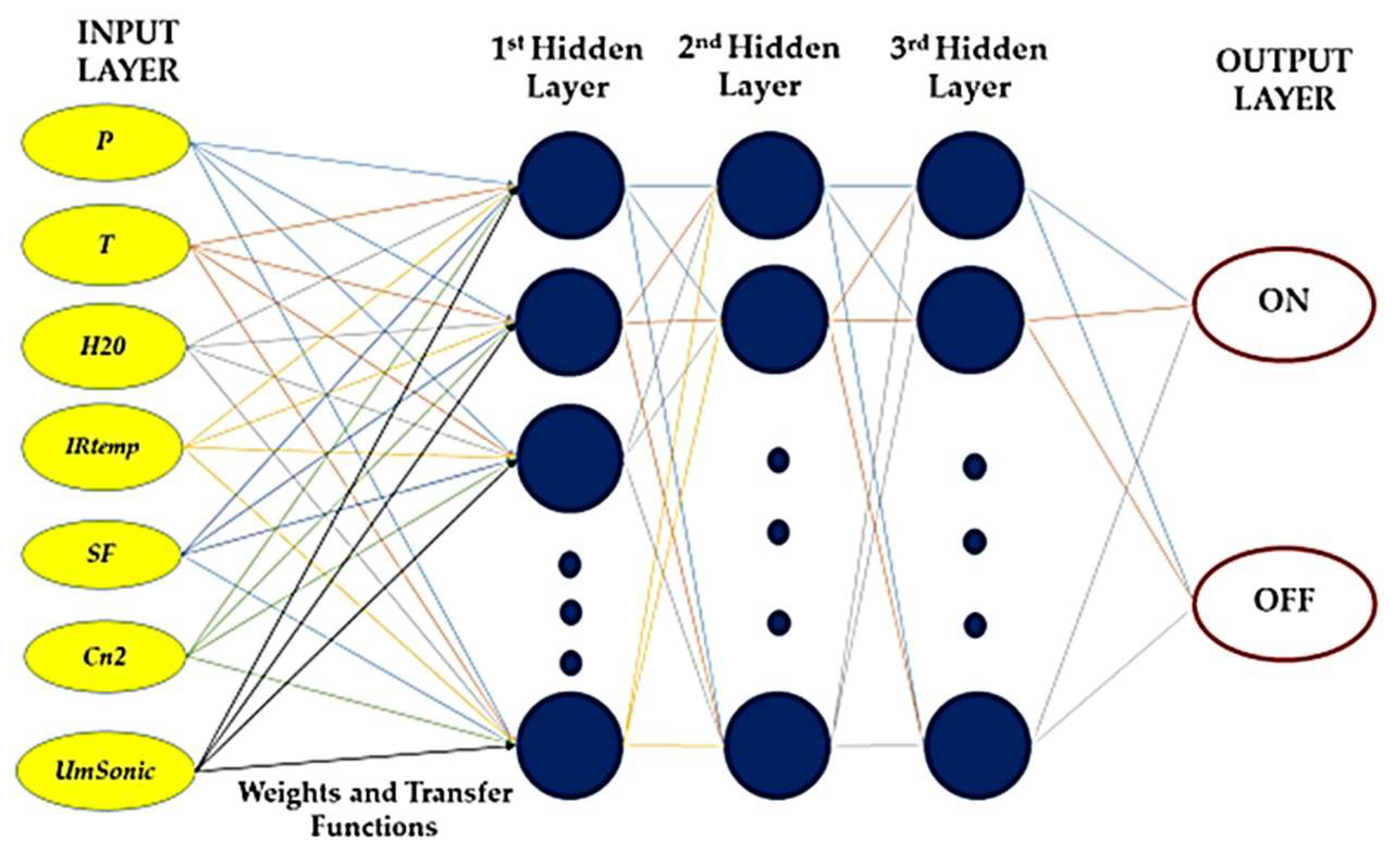
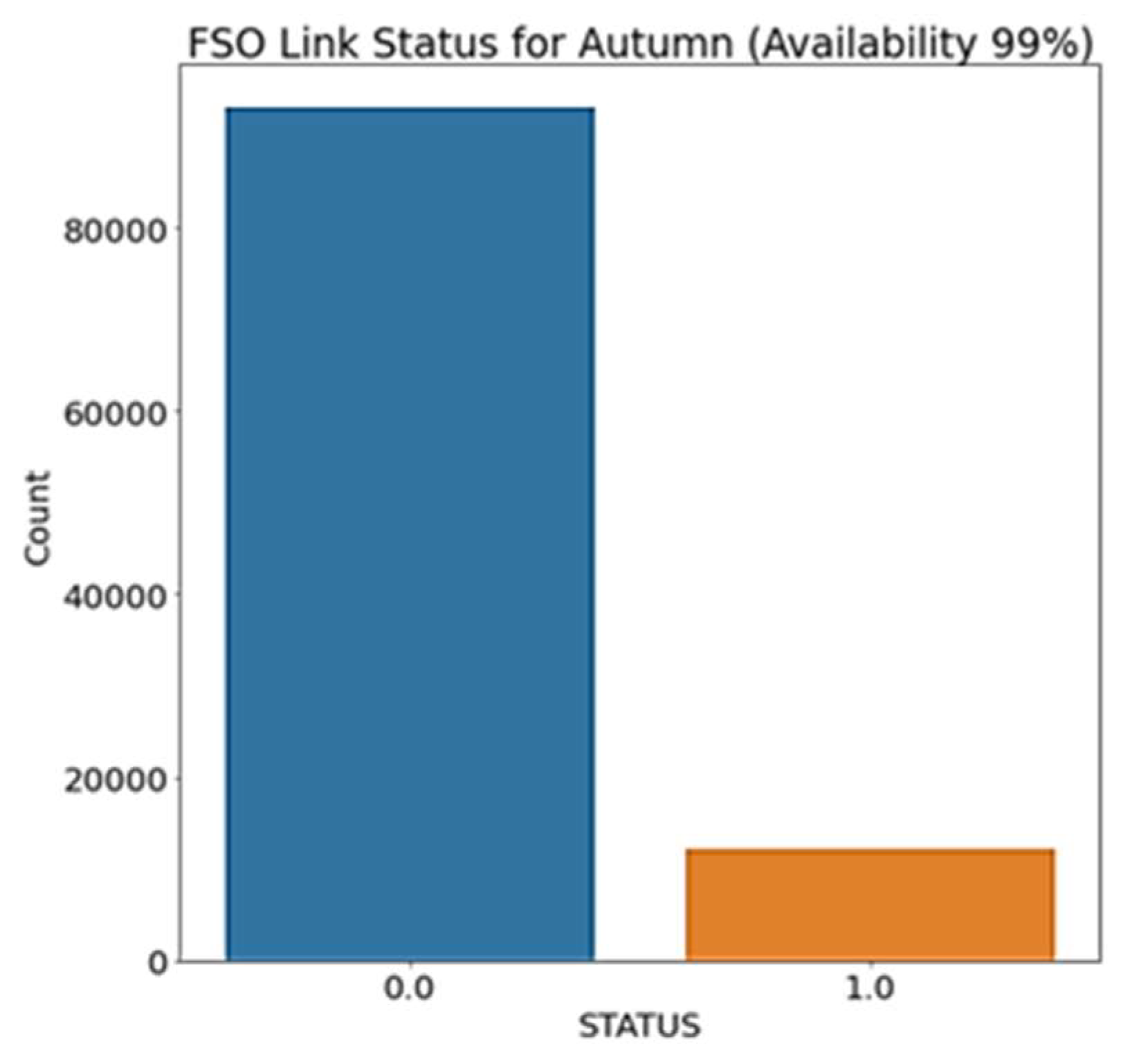
A received signal below a certain threshold level in an FSO link would eventually result in fading and perhaps a total link interruption. This section aims to present a DNN approach to model the status of a notional FSO link, that is either functional (On) or non-functional (Off) in the laser mode. That way, we can be able to predict the status of the link, whether it will operate in the laser or radio frequency mode for a hybrid installation. To do so, we utilized the environmental data set per season as described in Section 4.1 and built a deep neural network (Figure 11) to classify the link’s operational status as functional (On) or Non-functional (Off). The inputs used were air temperature (T), wind speed (UmSonic), water vapor concentration (H2O), solar flux (SF), air pressure (Pair), ground temperature (IRtemp) and the refractive index structure parameter (). We assumed a required 99% availability for our link (or, equivalently, an outage probability more than Pout = 0.01). Therefore, a “0” was attached to every row in our dataset with Pout > 0.01 and a “1” for Pout < 0.01. The resulting split of our experimental data for all seasons was quite unbalanced and showed that most of the observations imply a non-functional state for laser operational mode of the notional FSO. However, it gives interesting insights on a realistic operational performance of an FSO link. Figure 12 presents the results on the “0” (non-functional, off state) and “1” (functional, on state) of the link. A similar pattern was followed for the other three seasons as well.

Figure 11.
The Deep Neural Network approach to classify the FSO link laser mode status.
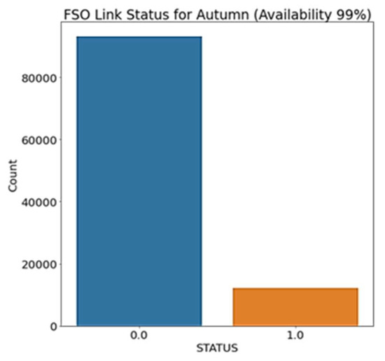
Figure 12.
The cumulative results of the FSO operational status for the Autumn season. “0” for non-functional and “1” for functional laser operation.
The DNN classification network has three hidden layers with 50, 30 and 10 neurons, respectively. A feed-forward back propagation algorithm was used, with a dropout rate of 0.5 per layer. The activation function for the three hidden layers was a rectifier (ReLU) whereas for the output layer a sigmoid function was used. In order for the algorithm to monitor the progress of the fitting, a binary cross entropy loss function was used, and the Adam optimizer was used to adapt the gradient descent of the loss function. The algorithm was trained against 80% of the dataset and tested over the rest 20%. An early stopping criterion was also introduced to avoid overfitting the model, which lead to a total of 189 training epochs for a batch size of 32.
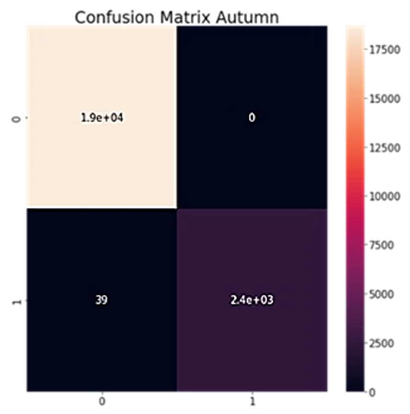
Figure 13 shows the progressive performance of the model throughout training, measured by the accuracy and loss both for the training and the validation set. The model exhibits a significant accuracy early on the epochs iteration, which after slight variations seems to stabilize after around 150 epochs. The early stopping criterion interrupted training at the 189th epoch. Figure 14, presents the confusion matrix of the DNN classification model. By definition a confusion matrix C is such that Ci,j is equal to the number of observations known to be in group i and predicted to be in group j. Thus, in a binary classification the count of true negatives is C0,0, false negatives is C1,0, true positives is C1,1 and false positives is C0,1. As shown in Figure 13, we confirmed the excellent classification performance of the DNN, since we observe that false negatives C1,0 = 0 and false positives is C0,1 = 39, which means that out of the almost 2400 “1”s only 39 false predictions were made instead.
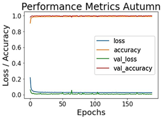
Figure 13.
The loss/accuracy performance of the deep neural classifier for the Autumn season. An early stopping criterion interrupted the training after 189 epochs.

Figure 14.
The confusion matrix for the DNN classifier during Autumn.
4.5. Modeling Outage Probability
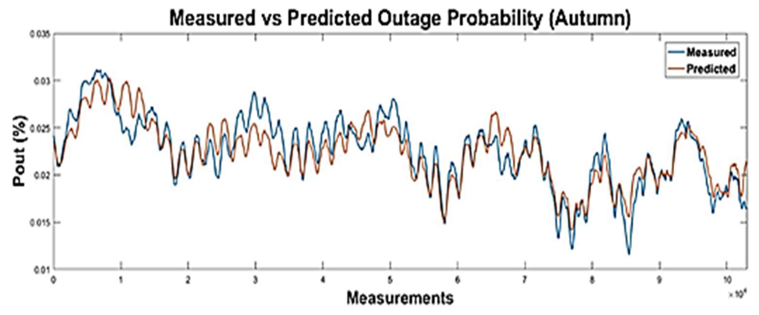
The last section of the paper aimed to develop an easily interpretable mathematical model for outage probability estimation, based upon routine meteorological parameters and refractive index. A first order polynomial has been selected to provide a decent fit among seven independent parameters, i.e., IR temperature, solar flux, atmospheric water concentration, air temperature, wind speed, atmospheric pressure and logarithmic refractive index structure parameter, and the dependent Pout to the autumn dataset with a coefficient, R2 = 0.55. The mathematical expression that gives the predicted outage probability is
Figure 15 plots the predicted values of Pout obtained from Equation (20) against the measured values obtained from Equation (18) for the autumn dataset. The daily mean value—instead of raw data—for both values has been used for a clearer depiction. We notice that the model’s predictions follow the general trend of the experimental Pout, thus it can be used to give very good estimates for the performance of an FSO link.
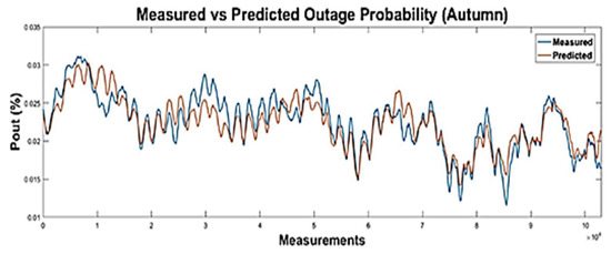
Figure 15.
Measured vs Predicted outage probability time series for autumn.
5. Conclusions
This paper is comprised of two main parts, which present a thorough analysis of and FSO outage probability modeling, by leveraging machine learning algorithms.
The first part of the paper presented the regression analysis results for . We utilized six common ML algorithms and trained them on four different data sets (i.e., one for each season) that consisted of six experimentally obtained macroscopic meteorological parameters for inputs. The results showed a large variation on the prediction accuracy between each model. Specifically, the ANN algorithm showed a moderate to low accuracy, with R2 = 0.55 and RMSE = 0.0916. The RF algorithm gave a significantly improved coefficient of determination for the model evaluation, R2= 0.78, which was the best value among all algorithms for every season. Additionally, an RMSE = 0.064 showed a great improvement in the error of the predicted values. The GBR model was comparable to the RF model by achieving a value of R2 = 0.7 and an RMSE = 0.075. The KNN resulted in R2 = 0.71 and an RMSE = 0.073. That is, it slightly outperformed the GBR algorithm. The DT algorithm resulted in R2 = 0.637 and RMSE = 0.083. Finally, the DNN algorithm resulted in an R2 = 0.61 and an RMSE = 0.085.
Previous studies on exploiting ML algorithms for prediction exist [29,30]. In [29], two ML algorithms (Random Forest and Boosted Trees) were trained on experimentally obtained observations over a maritime environment. Although this work utilized a scintillometer to measure the refractive index structure parameter, which is a path averaged value, we notice that the superiority of the RF algorithm in terms of prediction accuracy is consistent with out results. However, that work used a different performance metric than this paper—namely, it used the mean absolute error (MAE). In this paper, we applied the RMSE and the coefficient of determination, R2. Therefore, no direct comparison can be made. Furthermore, only two ML algorithms were used, so no validation could be made referring to the rest four ML algorithms used in this paper. In [30], a ANN model is used to estimate the value of . However, the results presented refer to the 50th percentile of values and showed a very good agreement with the measured values (R2 ~ 0.8).
The second part of the paper was devoted on a thorough analysis for the outage probability of a notional FSO link. Initially, the corresponding Pout for the measured meteorological conditions was derived based on an existing in the literature mathematical formula. These Pout estimations were used to classify the link status as functional or non-functional depending on a required availability of 99%, which corresponds to a 1% outage probability. We then trained a DNN classifier to model the status of the link based on six measured meteorological parameters as inputs. Finally, we developed a simple mathematical model for outage probability estimation based upon those meteorological parameters and refractive index. Both the DNN classifier and the regression formula showed a very good performance. To the authors’ knowledge, an experimentally obtained outage probability analysis for an FSO link does not exist in the literature, therefore the work presented in this paper is of significant importance to the FSO technology community.
The Hellenic Naval Academy (HNA), Piraeus, Greece, has demonstrated a substantial research effort on the field of atmospheric characterization and modeling with a focus on laser communication systems applications [3,4,5,21,26,31,32]. An established horizontal laser communication link between the roof of the HNA and the lighthouse of Psitalia island, 2958 m apart and 35 m above sea level, is utilized to measure the received signal strength on the receiver. Additional sensors, i.e., weather station, scintillometer, collect various atmospheric parameters such as air pressure, temperature, wind speed and direction, rainfall rate, dew point, solar flux and relative humidity, and refractive index structure related parameters (), such as the structure parameter of the temperature fluctuations (), the sensible heat flux, the scintillation index, the intensity and the Fried parameter. Within the next months, this data will be exploited in order to develop new, more efficient machine learning and deep learning algorithms to provide more accurate predictions, which will directly be compared against the measurements from a scintillometer (BLS-450) that is co-located with the FSO transceiver.
Author Contributions
Conceptualization, A.L., K.P., A.S. (Antonios Sklavounos), A.S. (Antonios Stassinakis) and K.C.; methodology, A.L., K.P., A.S. (Antonios Sklavounos) and K.C.; software, A.L., K.P., A.S. (Antonios Sklavounos), A.S. (Antonios Stassinakis) and A.T.; validation, A.L., K.P., H.N., A.T. and K.C.; formal analysis, A.L., A.S. (Antonios Sklavounos) and A.T.; investigation, A.L., K.P. and H.N.; resources, A.L., K.P., K.A. and A.T.; writing—original draft preparation, A.L., K.P. and A.T.; writing—review and editing, A.L., K.P., H.N., A.T., K.C. and K.A.; supervision, K.P., A.T., H.N. and K.C. All authors have read and agreed to the published version of the manuscript.
Funding
This research received no external funding.
Data Availability Statement
Available online: https://dx.doi.org/10.21227/8bqw-gy72 (accessed on 27 December 2022).
Conflicts of Interest
The authors declare no conflict of interest.
References
- Young, D.W.; Hurt, H.H.; Sluz, J.E.; Juarez, J.C. Development and Demonstration of Laser Communication Systems. Johns Hopkins APL Tech. Dig. 2015, 33, 122–138. [Google Scholar]
- Garlinska, M.; Pregowska, A.; Gutowska, I.; Osial, M.; Szczepanski, J. Experimental Study of the Free Space Optics Communication System Operating in the 8–12 m Spectral Range. Electronics 2021, 10, 875. [Google Scholar] [CrossRef]
- Lionis, A.; Peppas, K.; Nistazakis, H.E.; Tsigopoulos, A.D.; Cohn, K. Experimental Performance Analysis of an Optical Communication Channel over Maritime Environment. Electronics 2020, 9, 1109. [Google Scholar] [CrossRef]
- Lionis, A.; Peppas, K.; Nistazakis, H.E.; Tsigopoulos, A.D.; Cohn, K. Statistical Modeling of Received Signal Strength for an FSO Channel over Maritime Environment. Opt. Commun. 2020, 489, 126858. [Google Scholar] [CrossRef]
- Lionis, A.; Peppas, K.; Nistazakis, E.; Tsigkopoulos, A.; Cohn, K. RSSI probability density functions comparison using Jenshen-Shannon divergence and Pearson distribution. Technologies 2021, 9, 26. [Google Scholar] [CrossRef]
- Jellen, C.; Nelson, C.; Brownell, C.; Burkhardt, J.; Oakley, M. Measurement and analysis of atmospheric optical turbulence in a near-maritime environment. IOP SciNotes 2020, 1, 024006. [Google Scholar] [CrossRef]
- Wang, H.; Li, B.; Wu, X.; Liu, C.; Hu, Z.; Xu, P. Prediction model of atmospheric refractive index structure parameter in coastal area. J. Mod. Opt. 2015, 62, 1336–1346. [Google Scholar] [CrossRef]
- Basu, S. A simple approach for estimating the refractive index structure parameter (Cn2n) profile in the atmosphere. Opt. Lett. 2015, 40, 4130–4133. [Google Scholar] [CrossRef]
- Marzano, F.S.; Mori, S.; Frezza, F.; Nocito, P.; Beleffi, G.T.; Incerti, G.; Restuccia, E.; Consalvi, F. Free-space optical high-speed link in the urban area of southern Rome: Preliminary experimental set up and channel modelling. In Proceedings of the 5th European Conference on Antennas and Propagation (EUCAP), Rome, Italy, 11–15 April 2011; pp. 2737–2741. [Google Scholar]
- Rafalimanana, A.; Giordano, C.; Ziad, A.; Aristidi, E. Prediction of atmospheric turbulence by means of WRF model for optical communications. In Proceedings of the International Conference on Space Optics—ICSO 2021, Online, 30 March–2 April 2021; Volume 11852. [Google Scholar] [CrossRef]
- Dmytryszyn, M.; Crook, M.; Sands, T. Lasers for Satellite Uplinks and Downlinks. Sci 2021, 3, 4. [Google Scholar] [CrossRef]
- Trinh, P.V.; Carrasco-Casado, A.; Okura, T.; Tsuji, H.; Kolev, D.; Shiratama, K.; Munemasa, Y.; Toyoshima, M. Experimental Channel Statistics of Drone-to-Ground Retro-Reflected FSO Links With Fine-Tracking Systems. IEEE Access 2021, 9, 137148–137164. [Google Scholar] [CrossRef]
- Mishra, P.; Sonali; Dixit, A.; Jain, V.K. Machine Learning Techniques for Channel Estimation in Free Space Optical Communication Systems. In Proceedings of the IEEE International Conference on Advanced Networks and Telecommunications Systems (ANTS), Goa, India, 16–19 December 2019; pp. 1–6. [Google Scholar] [CrossRef]
- Vorontsov, A.M.; Vorontsov, M.A.; Filimonov, G.A.; Polnau, E. Atmospheric Turbulence Study with Deep Machine Learning of Intensity Scintillation Patterns. Appl. Sci. 2020, 10, 8136. [Google Scholar] [CrossRef]
- Lohani, S.; Knutson, E.M.; Glasser, R.T. Generative machine learning for robust free-space communication. Commun. Phys. 2020, 3, 177. [Google Scholar] [CrossRef]
- CLamprecht; Bekhrad, P.; Ivanov, H.; Leitgeb, E. Modelling the Refractive Index Structure Parameter: A ResNet Approach. In Proceedings of the 2020 International Conference on Broadband Communications for Next Generation Networks and Multimedia Applications (CoBCom), Graz, Austria, 7–9 July 2020; pp. 1–4. [Google Scholar] [CrossRef]
- Wang, Y.; Basu, S. Estimation of optical turbulence in the atmospheric surface layer from routine meteorological observations: An artificial neural network approach. In Proceedings of the SPIE Optical Engineering + Applications, San Diego, CA, USA, 17–21 August 2014; Volume 9224. [Google Scholar] [CrossRef]
- Xiong, W.; Wang, P.; Cheng, M.; Liu, J.; He, Y.; Zhou, X.; Xiao, J.; Li, Y.; Chen, S.; Fan, D. Convolutional Neural Network Based Atmospheric Turbulence Compensation for Optical Orbital Angular Momentum Multiplexing. J. Lightwave Technol. 2020, 38, 1712–1721. [Google Scholar] [CrossRef]
- Vint, D.; Di Caterina, G.; Soraghan, J.; Lamb, R.; Humphreys, D. Analysis of deep learning architectures for turbulence mitigation in long-range imagery. In Proceedings of the SPIE Security + Defence, Online, 21–25 September 2020; Volume 11543. [Google Scholar] [CrossRef]
- Amirabadi, M.A. A survey on machine learning for optical communication [machine learning view]. arXiv 2019, arXiv:1909.05148. [Google Scholar]
- Lionis, A.; Peppas, K.; Nistazakis, H.E.; Tsigopoulos, A.; Cohn, K.; Zagouras, A. Using Machine Learning Algorithms for Accurate Received Optical Power Prediction of an FSO Link over a Maritime Environment. Photonics 2021, 8, 212. [Google Scholar] [CrossRef]
- Andrews, L.C.; Phillips, R.L.; Hopen, C.Y. Laser Beam Scintillation with Applications, 2nd ed.; SPIE Optical Engineering Press: Bellingham, WA, USA, 2001. [Google Scholar]
- Kaushal, H.; Jain, V.K.; Kar, S. Free-Space Optical Channel Models. In Free Space Optical Communication; Optical Networks; Springer: New Delhi, India, 2017; pp. 41–89. [Google Scholar] [CrossRef]
- Nistazakis, H.; Katsis, A.; Tombras, G. On the Reliability and Performance of FSO and Hybrid FSO Communication Systems over Turbulent Channels. In Turbulence: Theory, Types and Simulation; Grove Press: New York, NY, USA, 2012. [Google Scholar]
- Prudnikov, A.P.; Brychcov, Y.A.; Marichev, O.I. Integrals and Series Volume 3: More Special Functions, 1st ed.; Gordon and Breach Science Publisher: Philadelphia, PA, USA, 1986. [Google Scholar]
- Lionis, A.; Chaskakis, G.; Cohn, K.; Blau, J.; Peppas, K.; Nistazakis, H.E.; Tsigopoulos, A. Optical Turbulence Measurements and Modeling Over Monterey Bay. Opt. Commun. J. 2022, 520, 128508. [Google Scholar] [CrossRef]
- Sklavounos, A. Measurements of Optical Turbulence and Analysis using Machine Learning. Master’s Thesis, Naval Postgraduate School, Monterey, CA, USA, 2021. [Google Scholar]
- Lionis, A.; Peppas, K.; Tsigkopoulos, A.; Sklavounos, A.; Stasinakis, A.; Nistazakis, H.; Kohn, K.; Aidinis, K. Experimental Machine Learning Approach for Optical Turbulence and FSO Outage Performance Modeling. IEEE DataPort 2022. [Google Scholar] [CrossRef]
- Jellen, C.; Oakley, M.; Nelson, C.; Burkhardt, J.; Brownell, C. Machine-learning informed macro-meteorological models for the near-maritime environment. Appl. Opt. 2021, 60, 2938–2951. [Google Scholar] [CrossRef]
- Wang, Y.; Basu, S. Using an artificial neural network approach to estimate surface-layer optical turbulence at Mauna Loa, Hawaii. Opt. Lett. 2016, 41, 2334–2337. [Google Scholar] [CrossRef]
- Lionis, A.; Tsigopoulos, A. High Energy Laser Weapon Integration Issues for the Future Hellenic Frigate. Nausivios Chora J. 2022. [Google Scholar]
- Lionis, A.; Tsigopoulos, A.; Keith, C. An Application of Artificial Neural Networks to Estimate the Performance of High-Energy Laser Weapons in Maritime Environments. Technologies 2022, 10, 71. [Google Scholar] [CrossRef]


Disclaimer/Publisher’s Note: The statements, opinions and data contained in all publications are solely those of the individual author(s) and contributor(s) and not of MDPI and/or the editor(s). MDPI and/or the editor(s) disclaim responsibility for any injury to people or property resulting from any ideas, methods, instructions or products referred to in the content. |
© 2023 by the authors. Licensee MDPI, Basel, Switzerland. This article is an open access article distributed under the terms and conditions of the Creative Commons Attribution (CC BY) license (https://creativecommons.org/licenses/by/4.0/).