In this section, the dataset and implementation details are introduced, and then some experimental procedures of our method are introduced. Second, quantitative and qualitative comparisons were conducted using traditional feature-based and deep learning-based methods on a synthetic benchmark dataset to demonstrate the performance of our method. Traditional feature-based methods include nine methods consisting of five feature descriptors (SIFT [
8]/ORB [
10]/BRISK [
18]/AKAZE [
19]/KAZE [
20]) and two outlier rejection algorithms (RANSAC [
11]/MAGSAC++ [
13]) combined. In particular, the KAZE [
20] + MAGSAC++ [
13] algorithm has difficulty in obtaining homography matrices in infrared and visible scenes, so it was not used as a comparison method. Deep-learning-based methods include UDHN [
14], CADHN [
15], MBL-UDHEN [
16], and HomoGAN [
17]. In particular, UDHN [
14] is difficult to fit in infrared and visible scenarios. MBL-UDHEN [
16] and HomoGAN [
17] both use the idea of homography flow, but the large grayscale and contrast differences in the infrared and visible images themselves cause the homography flow to become unstable, making it difficult for the network to converge. Therefore, we only make a comparison with CADHN [
15] in the subsequent qualitative comparison and quantitative comparisons. Finally, analytical results from some ablation experiments are provided to demonstrate the effectiveness of shallow feature extraction networks and generator backbones with unshared weights.
4.3. Comparison on Synthetic Benchmark Dataset
Qualitative comparison. Qualitative comparisons were performed with ten contrasting methods in the synthetic benchmark dataset, including feature-based methods and deep learning-based methods.
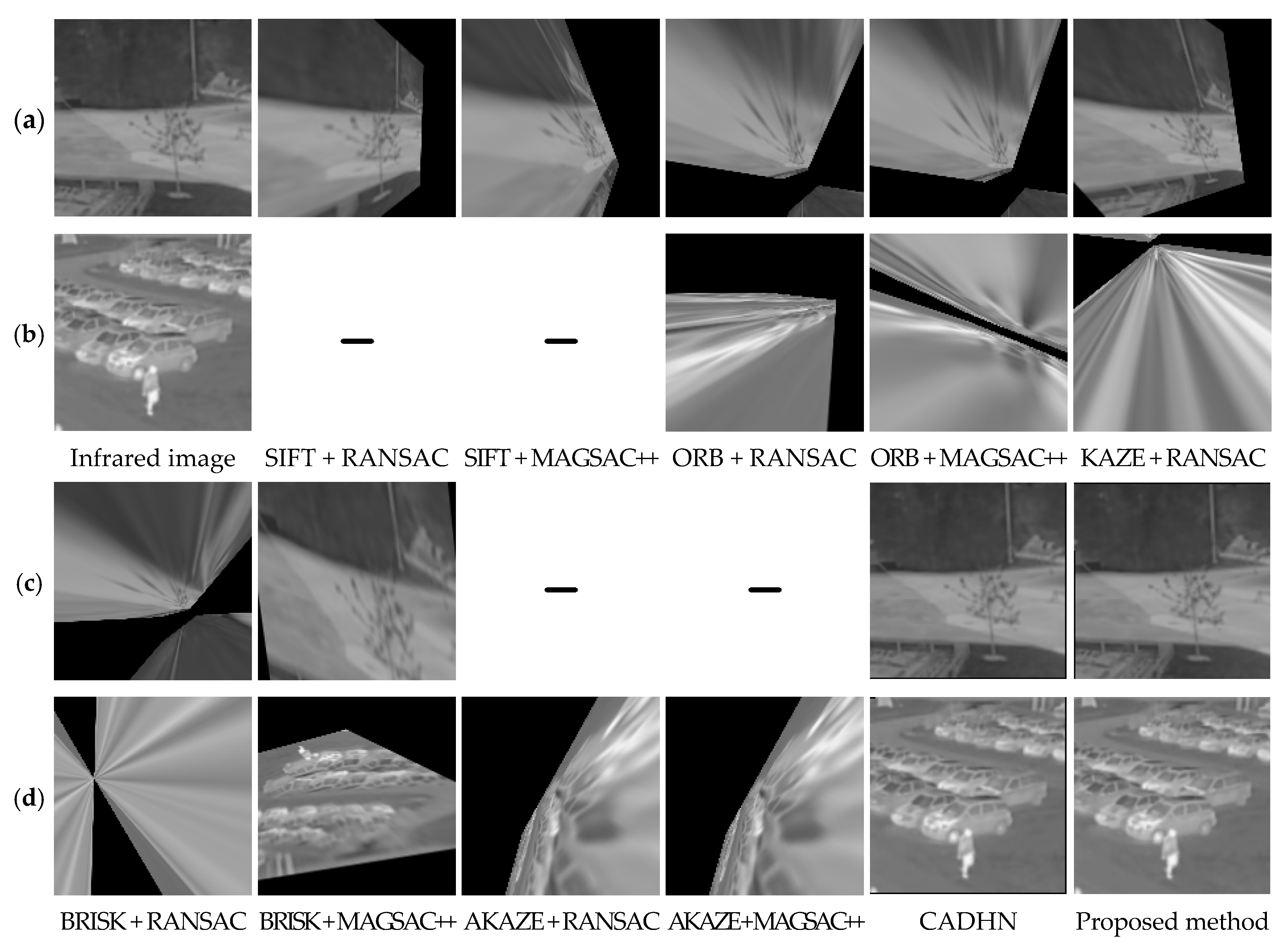
Figure 8 shows the comparison of the warped images obtained by using different methods based on the homography matrix, where “-” indicates that the algorithm failed. It can be seen that the feature-based methods have serious distortion and algorithm failure compared to the deep learning-based methods. In particular, SIFT [
8] and AKAZE [
19] appear to experience algorithm failures under these two examples. The deep learning-based methods have no distortion, and it is difficult to see the obvious difference between CADHN [
15] and the proposed method.
To distinguish the unregistered region between the warped and the ground-truth image clearly, channel mixing was performed on them to more intuitively reflect the homography estimation performance, as shown in
Figure 9. It can be seen that our method significantly outperforms the rest of the comparison methods. Specifically, in
Figure 9a,c, SIFT [
8] + RANSAC [
11] is the best-performing method among the feature-based methods but slightly worse than our method. In particular, there are more unaligned regions in the deep learning-based method CADHN [
15] than SIFT [
8] + RANSAC [
11], but CADHN [
15] does not appear to exhibit algorithm failure, so feature-based methods are difficult to apply to actual scenarios. The failure of the algorithm can be observed in the quantitative comparison. For example, the curve of the method SIFT [
8] + RANSAC [
11] is not smooth enough and has an obvious ladder shape, as seen in
Figure 10. For
Figure 9b,d, the deep learning-based methods are better than the feature-based methods. All feature-based methods suffer from significant ghosting, i.e., most of the regions are misaligned. Although it is difficult to distinguish the proposed method from CADHN [
15] in the channel mixing results, the superiority of the proposed method can be observed in subsequent quantitative comparisons.
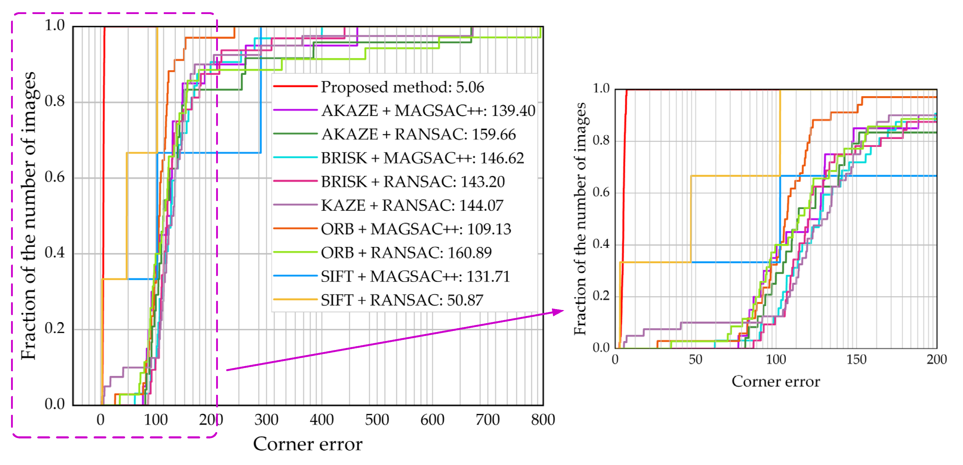
Quantitative comparison. Figure 10 shows the quantitative comparison of our method with the feature-based methods in the synthetic benchmark dataset. As shown in
Figure 10, the corner error [
31] of the proposed HomoMGAN method is much lower than that in the feature-based method, showing superior performance in infrared and visible scenes. In particular, SIFT [
8] + RANSAC [
11] and SIFT [
8] + MAGSAC++ [
13] both show three ladders, which is because they only predict homography matrices on three images. Specifically, if algorithm failure occurs in multiple test images, the fraction of the number of images in a larger range remains unchanged at a certain value of corner error [
31] in
Figure 10, i.e., a ladder shape appears. Although SIFT [
8] + RANSAC [
11] fails in most test images in
Figure 10, its corner error is the lowest among all of the traditional feature-based methods, confirming the conclusion in the qualitative comparison. In addition, the evaluation values of the remaining eight feature-based methods are close, so we locally zoom in on them, as shown on the right side in
Figure 10. We can see that the performance of ORB [
10] + MAGSAC++ [
13] is the best among these eight methods, but the performance of ORB [
10] + RANSAC [
11] is the worst. At the same time, it is not difficult to see that the feature-based methods have ladders to varying degrees, i.e., the homography matrix cannot be predicted in some test images, but the proposed HomoMGAN method does not experience algorithm failure.
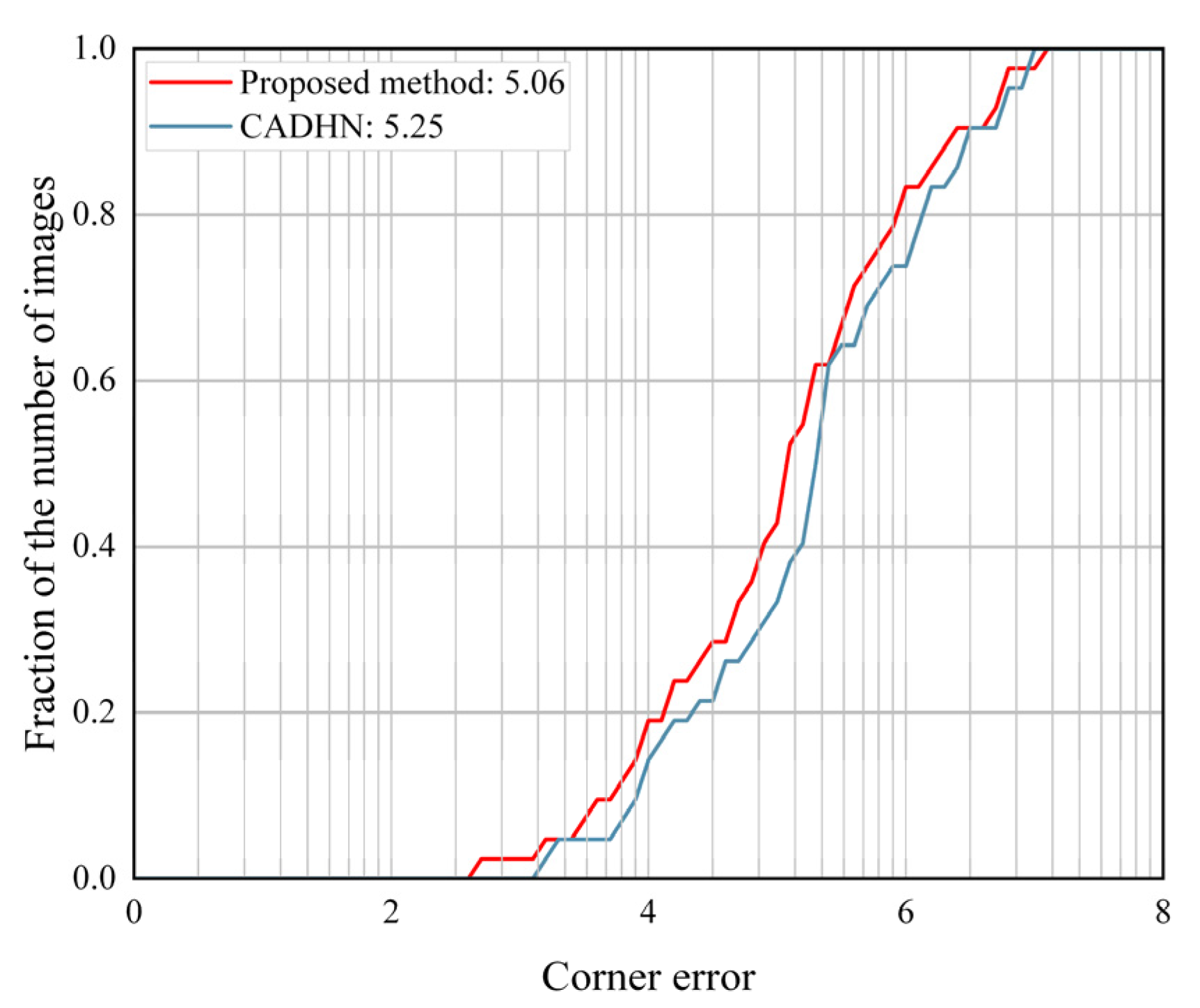
Figure 11 shows the quantitative comparison of our method with the deep learning-based methods in the synthetic benchmark dataset. As shown in
Figure 11, the proposed HomoMGAN method achieves the best performance among deep learning-based methods and significantly outperforms CADHN [
15]. According to the trend in the figure, HomoMGAN has a lower corner error [
31] than CADHN [
15] for most of the test images.
Discussions. The synthetic benchmark dataset comes from several real-world outdoor scenes, including parking lots, schools, parks, etc. After experimental verification, our method can obtain a more accurate homography matrix in these scenarios, and the registration effect is more reasonable. Since the essence of our synthetic benchmark dataset comes from registered real-world datasets, which to some extent reflect the unregistered situation of real-world data, our method also effectively performs when using unregistered real-world datasets.
4.4. Ablation Experiment
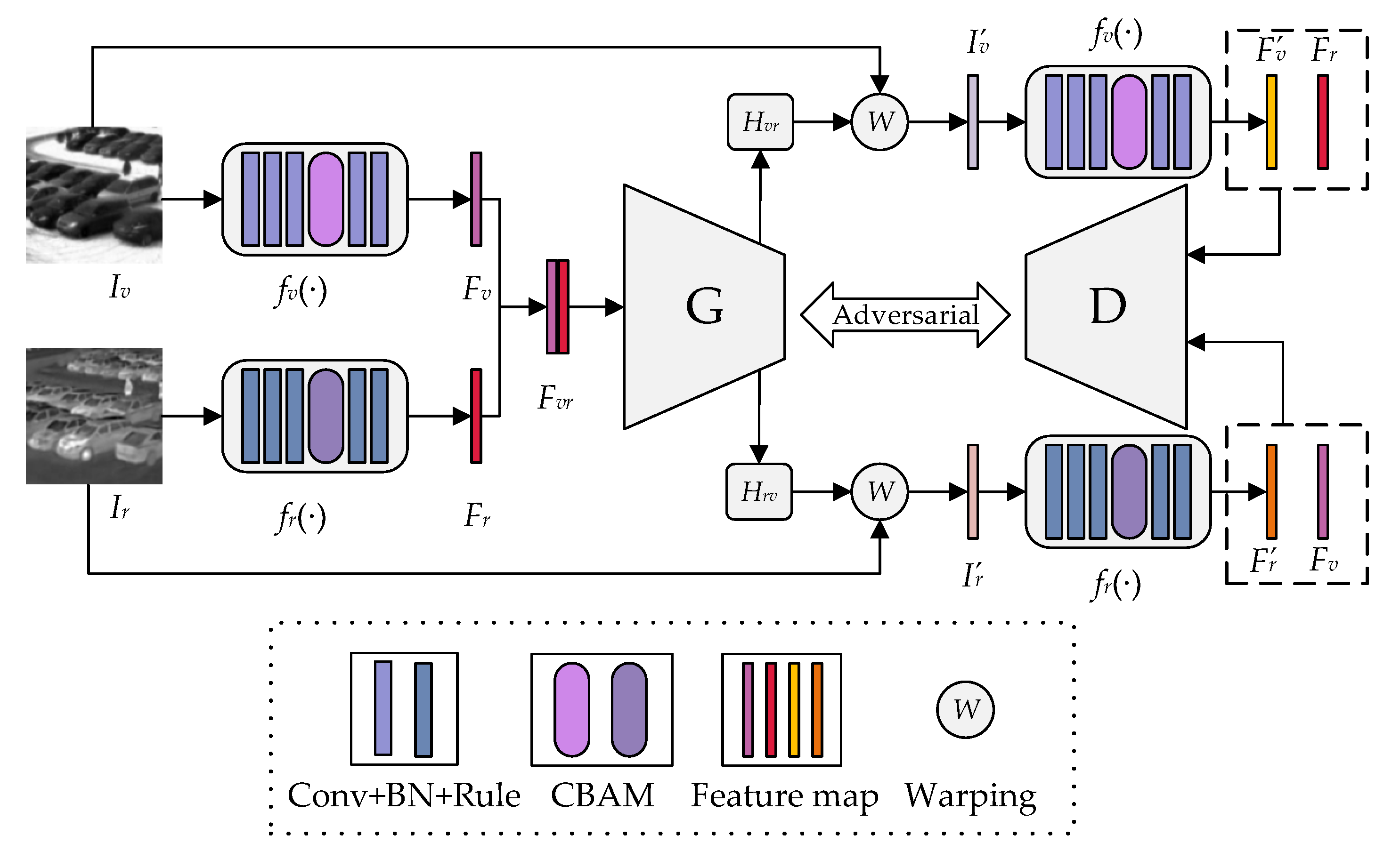
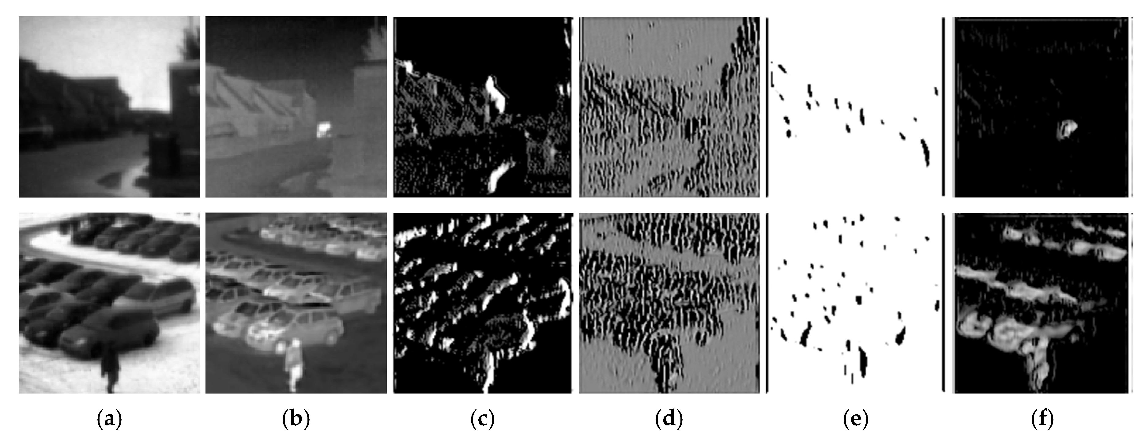
Shallow feature extraction network. The effectiveness of the shallow feature extraction networks was mainly verified from two perspectives relating to the synthetic benchmark dataset. First, the shallow feature extraction network was replaced with the feature extractor and mask predictor [
15], whose feature map comparison is shown in
Figure 12. The main reason that this replacement was undertaken is that they function similarly; they both obtain weighted feature maps, highlighting features that are meaningful for homography estimation. As shown in
Figure 12, it can be seen that the feature maps produced by our shallow feature extraction network are sparser, which is beneficial in reducing the noise in the feature maps. To prove the effectiveness of our shallow feature extraction network more clearly, we show the corner error [
31] of two sample image pairs in
Figure 12, as shown in
Table 2. It can be seen in
Table 2 that the corner error [
31] of the shallow feature extraction network on both sets of sample image pairs is much lower than that of the feature extractor and mask predictor [
15], proving that the sparse features in our method can effectively reduce the noise in the feature map, improving the accuracy of the homography matrix. In order not to lose generality, we also compare the average corner error [
31] on the test set of the feature extractor and mask predictor [
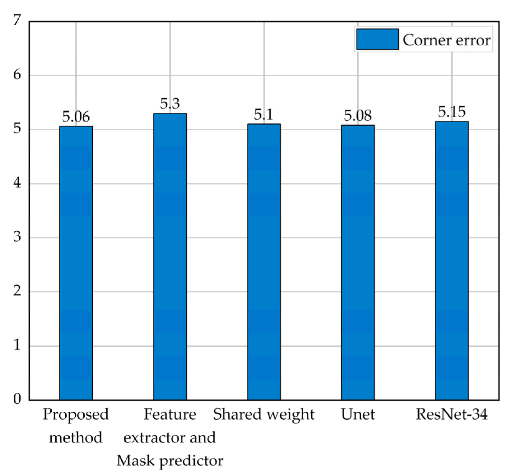
15] and shallow feature extraction network; the result is shown in
Figure 13. It can be seen that the homography estimation performance of our method is significantly better than that of the feature extractor and mask predictor [
15], fully confirming the effectiveness of our shallow feature extraction network. In addition,
Table 3 shows the comparison of the number of parameters and computations before and after replacing the shallow feature extraction network, and the results are shown in rows 2 and 3 in
Table 3, respectively. Although the number of parameters and computation of the proposed method is slightly higher than the results in row 3, the corner error of the proposed method is significantly lower than that in row 3 (from 5.3 to 5.06).
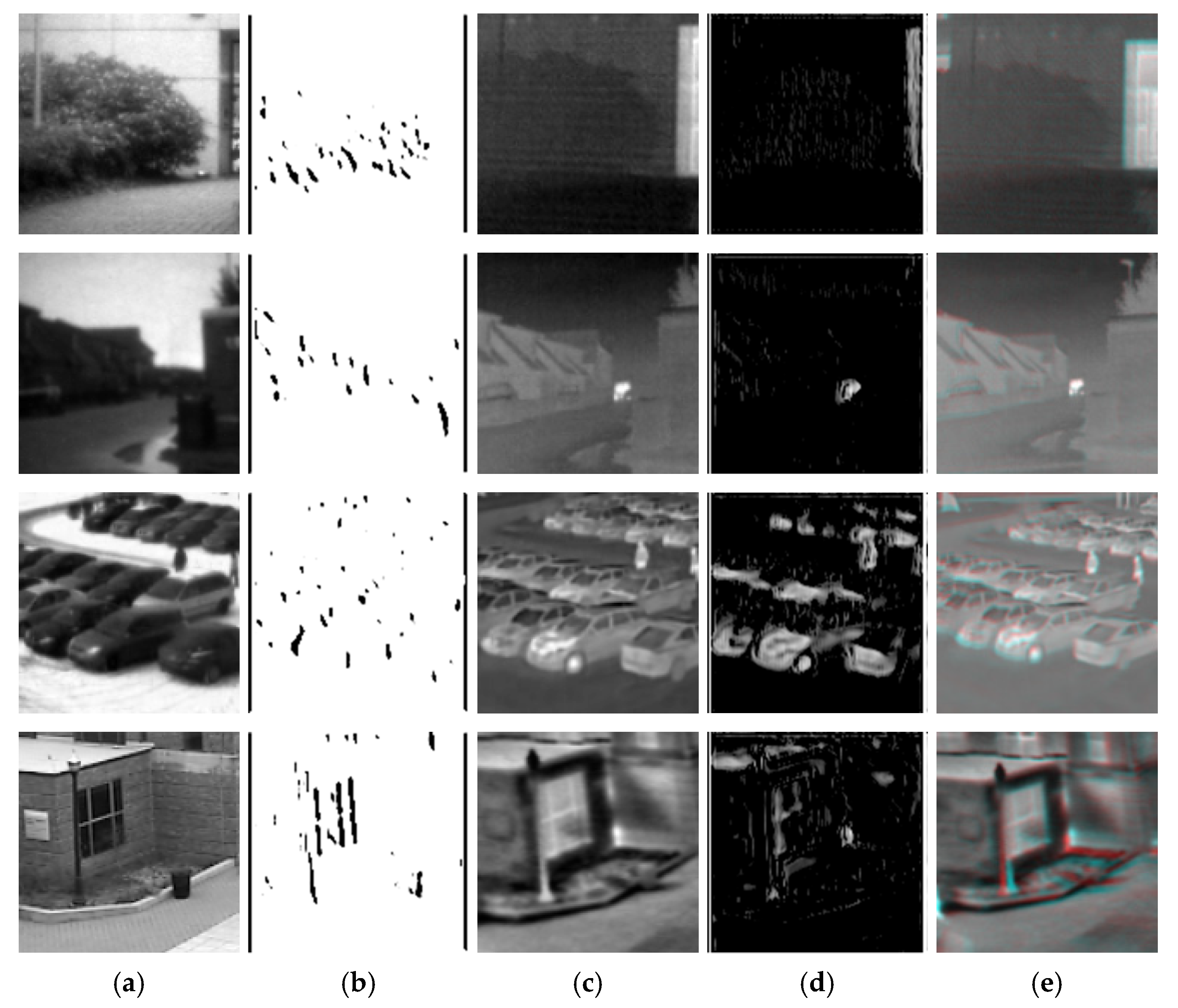
Second, the two conditions of the shallow feature extraction network were compared—”shared weight” and “w/o. shared weight” (the proposed method)—and the fine-feature map results are shown in
Figure 14. We show the output of the shallow feature extraction network to analyze the impact of “shared weight” and “w/o. shared weight” on the shallow feature extraction network. As shown in
Figure 14c,d, under the condition of shared weight, the fine-feature map output by the shallow feature extraction network retains a large number of dense features. However, this introduces significant noise into the homography estimation process, degrading homography estimation performance. Interestingly, after we no longer share the weight for the shallow feature extraction network, the network can extract features according to the imaging characteristics of each type of image, thereby reducing the impact of noise in homography estimation, as shown in
Figure 14e,f. In the case of “w/o. shared weight”, both the infrared image and the visible image not only retain meaningful features for homography estimation, but the number of features is significantly less than that under the “shared weight” conditions. The corner error [
31] in
Table 4 also demonstrates the advantage of “w/o. shared weight”; the corner error [
31] of “w/o. shared weight” is significantly lower than that of “shared weight” in these two sets of images. Similarly, as seen in
Figure 13, “w/o. shared weight” can significantly reduce the error from 5.1 to 5.06 compared with “shared weight”, which also proves the effectiveness of the shallow feature extraction network in our method without shared weight. In addition,
Table 3 compares the number of parameters and computations of “w/o. shared weight” and “shared weight”, as shown in rows 2 and 4 in
Table 3. The parameter amount in row 2 is slightly lower than in row 4, but its computation amount is slightly higher than in row 4.
Generator backbone. Several common backbones were investigated, including Unet [
38] and ResNet-34 [
39], to verify the effectiveness of the generator backbone in the proposed method. As shown in
Figure 12, our method achieves the best performance among these several backbones and slightly outperforms Unet [
38]. The homography estimation generator of the proposed method and Unet [
38] use the encoder–decoder structure to fuse shallow low-level features in the deep network, and the corner error of both is better than ResNet-34 [
39]. This fully illustrates that shallow low-level features can effectively improve homography estimation performance. Interestingly, Unet [
38] can be used to directly predict the homography matrix, and the performance is significantly better than the common backbone (ResNet-34 [
39]) in typical homography estimation methods [
15,
16]; the corner error [
31] dropped significantly from 5.15 to 5.08. To the best of our knowledge, Unet [
38] has not been used to directly predict homography matrices before. In addition,
Table 3 shows the comparison of the parameter amount and computation amount before and after generator backbone replacement, as shown in rows 2, row 5, and row 6 in
Table 3. Although ResNet-34 [
39] has the smallest number of parameters and computations, it has the highest corner error compared to the backbones.


