An Interference-Aware Resource-Allocation Scheme for Non-Cooperative Multi-Cell Environment

Abstract

Inter-cell interference cancellation has been investigated for several decades and has become an elementary technique for modern wireless networks. However, the existing interference cancellation mechanism rarely considers the historical channel variations and interference characteristics. In this paper, we propose an interference-aware prediction-based resource-allocation strategy to deal with multi-cell interference, where the historical noisy channel state and the acknowledgment feedback are fully utilized. Together with the predicted interference patterns, our proposed joint sub-channel allocation and rate selection mechanism can achieve better average throughput performance. Through the numerical as well as the prototyping results, we show that our proposed scheme is able to provide more than 9.7% and 8% average throughput improvement compared with many existing baselines.

1. Introduction

Due to the scarcity of wireless resources and economic considerations, different base stations (BSs) or cells work in the same frequency band, which is widely used in 4G and 5G. Inter-cell interference is caused between a frequency channel in one cell and the same frequency channel used in another adjacent cell. It is one of the most critical limitations to improving the effective throughput of cell edge user equipment (UE) [1], which has led to dozens of research efforts over the past several decades. With full channel state information (CSI) from the signal and interfering links, interference-alignment [2] or -mitigation [3] techniques have been extensively studied to reduce the interference level and achieve further throughput improvement. By utilizing a cooperative transmission strategy from all or part of the neighboring base stations, coordinated multi-point transmission (CoMP) [4] or coordinated beamforming [5] are shown to be beneficial to reduce the interference power as well. Since the complete CSI knowledge of all the signal and interference links is in general difficult to obtain in practical network deployment, the aforementioned interference management schemes suffer from the residual interference generated by imperfect processing, and the resultant throughput improvement is often limited [6].

A systematical approach to deal with the inter-cell interference without cooperation among different BSs is the famous inter-cell interference cancellation (ICIC) scheme [7], where the instantaneous inter-cell interference is measured and reported by the target UE, and the neighboring cells are scheduled to reduce the radiation power or transmit via different frequency reuse patterns. The similar interference cancellation strategy has been extended to the time domain by configuring almost blank subframes (ABS) [8], which is also known as enhanced ICIC (eICIC) in the third generation partnership project (3GPP) [9]. Based on ICIC and eICIC schemes, many promising technologies have been developed in recent years [10,11,12,13]. For example, in [10], the paper proposed a beam-based ABS allocation and beam-based cell range expansion (CRE) algorithm to reduce the interference on small cell edge users. With the formulation result, their scheme has a lower computation cost. In [11], the paper used CSI muting with time-domain thresholding to improve the spectral efficiency performance of the ICIC. In [12], the paper used the independent deep Q-learning method to control both the transmit power and beamforming in a distributed manner. The scheme can achieve the same system capacity as the traditional neural network algorithm without the training data. In [13], the paper proposed an approach for identifying opportunities for power transfer that integrate with existing protocols and infrastructures for eICIC. However, all the existing interference cancellation-based mechanisms rely on the channel feedback or uplink/downlink duality, and the historical channel variations are usually ignored. In addition, the inter-cell interference is often treated as a whole, and the detailed interference characteristics have not been fully exploited.

In order to fully utilize the above information and provide a valuable design guideline for practical interference management, we propose an interference-aware prediction-based resource-allocation strategy for non-cooperative multi-cell transmission, where the novelties are summarized as follows:

• Historical information utilization. Different from the conventional interference cancellation-based schemes [7], we propose to collect and store the historical noisy channel states and the acknowledgment/negative acknowledgment (ACK/NACK) feedback from UEs. With this historical information, we can predict the upcoming channel condition and determine the efficient resource allocation strategy accordingly.
• Interference pattern prediction. In addition, we also propose to predict the upcoming interference patterns based on the UEs feedback, where the historical threshold-based interference condition has been utilized. Based on the predicted interference patterns for different UEs, we are able to select the preferred UE-subchannel pairs with less interfering probability.
• Joint sub-channel allocation and rate selection. By utilizing the historical information and the predicted interference patterns, we provide a joint sub-channel allocation and transmission rate selection strategy based on a reinforcement learning framework with deep Q-network (DQN).
• Prototype verification. In the meantime, we implement a prototyping system and sample the interference environment with multiple BSs. By collecting the practical measured channel variations of the entire network, we verify our proposed joint sub-channel allocation and transmission rate selection strategy accordingly. Through both numerical and prototyping examples, we show that it achieves more than 9.7% and 8% average throughput gain for different interference environments, if compared with conventional schemes [14,15,16,17].

The rest of this paper is organized as follows. Section 2 introduces the system model. In Section 3, we introduce the protocol of data transmission and propose the optimization problem. In Section 4, we transform the original optimization problem and propose a DQN-based solution. In Section 5, we compare the proposed interference-aware resource-allocation strategy with the baselines and analyze the performance, followed by the concluding remarks in Section 6.

2. System Models

In this section, we provide the mathematical models of wireless communication networks with inter-cell interference and identify the corresponding performance metrics.

2.1. Network Configuration and Transmission Models

Consider an OFDMA-based multi-cell communication environment with a target BS $B_0$ and $N_{BS}$ neighboring BSs, i.e., $B_1,\dots ,B_{N_{BS}}$, as shown in Figure 1a. In Figure 1a, we assume that the UEs are all connected to BS1. For UE1, its interfering base stations are BS2 and BS3, and the other base stations are not taken into account because they are too far away from UE1. For UE2, compared with BS2 and BS4, it is closer to BS3, so its interfering base station is only BS3. The interfering base stations of UE3 are considered BS3 and BS4, and for UE4 are BS5 and BS6. We come to the conclusion that in the multi-base station scenario, by sorting the distance between UE and neighboring cells, one or two cells with the nearest distance can be obtained as interference cells. Other complex inter-cell interference can be classified into these two cases. From Figure 1a, we abstract three adjacent base stations into an inter-cell interference scene, and the UE located in the center of the three base stations is likely to be interfered, as shown in Figure 1b. A cell edge UE [18] is receiving downlink transmission information through wireless interfering links, where the received signals at the i-th sub-channel on the time slot t, $y^i\left(t\right)$, are given by

$$\begin{array}{c}\hfill y^i\left(t\right)=h_0^i\left(t\right)x_0^i\left(t\right)+\sum _{b=1}^{N_{BS}}{h}_b^i\left(t\right){\mathcal{I}}_b^i\left(t\right)x_b^i\left(t\right)+n^i\left(t\right),\end{array}$$

(1)

where $h_0^i\left(t\right),x_0^i\left(t\right)$ and $h_b^i\left(t\right),x_b^i\left(t\right)$ denote the channel-fading coefficients and the transmitted signals from the target BS and the b-th neighboring BS to the cell edge user, respectively. ${\mathcal{I}}_b^i\left(t\right)$ denotes the interference indicator, which equals to 1 if the b-th neighboring BS is interfering on the i-th sub-channel at the time slot t and 0 otherwise. $n^i\left(t\right)$ represents the additive white Gaussian noise with zero mean and normalized variances. In this paper, the interference we consider is the inter-cell interference caused by the power of neighboring base stations, and the interference caused by other equipment is not considered. According to Shannon’s theory [14], the corresponding channel capacity is given by

$$\begin{array}{c}\hfill C\left(t\right)=\sum _{i\in {\Omega }_{SC}\left(t\right)}{log}_2\left(1+\frac{|h_0^i{\left(t\right)|}^2}{{\sum }_{b=1}^{N_{BS}}{\left|h_b^i\left(t\right)\right|}^2{\mathcal{I}}_b^i\left(t\right)+1}\right),\end{array}$$

(2)

where ${\Omega }_{SC}\left(t\right)$ denotes the collections of the selected sub-channel according to different allocation strategies. We normalize the transmit powers of the target BS and neighboring BSs to be unity, i.e., $\mathbb{E}\left[|x_0^i{\left(t\right)|}^2\right]=\mathbb{E}\left[|x_b^i{\left(t\right)|}^2\right]=1$ for all b, i, and t.

In the practical systems, the instantaneous channel fading coefficients, $\left\{h_0^i\left(t\right)\right\}$, are difficult to obtain in general, and the modulation and coding schemes (MCS) with equivalent transmission rate $R\left(t\right)$ as well as the selected sub-channels ${\Omega }_{SC}\left(t\right)$ are determined based on the historical channel coefficients from feedback or uplink–downlink duality and interference conditions. Mathematically, we have the following relation:

$$\begin{array}{ccc}\hfill \left(R\left(t\right),{\Omega }_{SC}\left(t\right)\right)& =& f(\{h_0^i(t-1)+\Delta h_0^i(t-1)\},{\sigma }_b,\hfill \\ & & \left\{{\mathcal{I}}_b^i(t-1)\right\}),\hfill \end{array}$$

(3)

where $f(·)$ denotes the rate mapping function and $\Delta h_0^i(t-1)$ is the additive noises due to the limited feedback patterns or mismatched uplink–downlink channel duality, and ${\sigma }_b$ denotes the normalization interfering channel coefficient from the b-th neighboring BS. With the above setting, the achievable average throughput over the total transmission duration T is given by

$$\begin{array}{ccc}\hfill \mathcal{R}& =& \frac{1}{T}\sum _{t=1}^{T}R\left(t\right)\times \mathcal{I}\left(R\left(t\right)\le C\left(t\right)\right),\hfill \end{array}$$

(4)

where $\mathcal{I}(·)$ is the indicator function, which equals 1 if the inner condition holds and 0 otherwise.

2.2. Channel and Interference Models

Without loss of generality, we assume that the normalized channel fading coefficients, $h_b^i\left(t\right)/{\sigma }_b$ (${\sigma }_b$ is the interference normalization coefficient, which can be obtained via the standard UE uplink report) and $h_0^i\left(t\right)$, follow a L-state Markov model as explained in [16] and the transition matrix $P_{\mathcal{H}}$ is given by

$$\begin{array}{ccc}\hfill {\mathrm{P}}_{\mathcal{H}}& =& \left[\begin{array}{ccc}{p}_{11}& \cdots & p_{1L}\\ \cdots & p_{l{l}^{\prime }}& \cdots \\ p_{L1}& \cdots & p_{LL}\end{array}\right],\hfill \end{array}$$

(5)

where each element $p_{l{l}^{\prime }}$ denotes the transition probability from the channel state l to $l^{\prime }$. Moreover, we consider the interference model to be Markovian as well [19], where the state transition matrix $Q_I$ is given by

$$\begin{array}{ccc}\hfill {\mathrm{Q}}_I& =& \left[\begin{array}{cc}{q}_{00}& q_{01}\\ q_{10}& q_{11}\end{array}\right],\hfill \end{array}$$

(6)

where $q_{cd}$ denotes the state transition probability from the interference state ${\mathcal{I}}_b^i(t-1)=c$ to ${\mathcal{I}}_b^i\left(t\right)=d$.

3. Protocol and Problem Formulation

In this section, we first introduce the protocol of data transmission, point out the possibility of interference detection to improve throughput optimization according to the protocol, and finally put forward the optimization problem.

3.1. Transmission Protocol

The entire transmission process can be generally divided into three stages as shown in Figure 2, namely user information collection, channel condition and interference prediction, and rate identification and transmission. For illustration purposes, we consider the t-th time slot in the following description.

• User Information Collection. During the time slot t, the cell edge UE reports the measured channel condition of different sub-channels, $\{h_0^i(t-1)+\Delta h_0^i(t-1)\}$, the interference condition from all the neighboring BSs, i.e., $\left\{{\mathcal{I}}_b^i(t-1)\right\}$, and $\mathcal{I}\left(R\right(t-1)\le C(t-1\left)\right)$ to the target BS via uplink channels. (In the practical implementation, ${\mathcal{I}}_b^i(t-1)$ can be obtained by comparing the measured RSRP from the b-th neighbouring BS with a pre-defined threshold, and $\mathcal{I}\left(R\right(t-1)\le C(t-1\left)\right)$ can be inferred from the conventional ACK/NACK information as defined in [20]. In addition, we model $\Delta h_0^i(t-1)$ here to incorporate the potential noises generated from local channel estimation or imperfect feedback transmission.) Here, we assume that the base station can receive the uplink information completely, that is, interference is not considered in the information feedback.
• Channel condition and interference prediction. Once the UE feedback is received, the target BS combines the current and historical $(L-1)$ feedback reports to predict the upcoming channel fading environment ${\widehat{h}}_0^i\left(t\right)$ and the interference condition ${\widehat{\mathcal{I}}}_b^i\left(t\right)$. The corresponding mathematical expressions are thus given by

  $$\begin{array}{ccc}\hfill {\widehat{h}}_0^i\left(t\right)& =& f_1(h_0^i(t-1)+\Delta h_0^i(t-1),\dots ,\hfill \end{array}$$

  $$\begin{array}{ccc}& & h_0^i(t-L)+\Delta h_0^i(t-L)),\hfill \end{array}$$

  (7)

  $$\begin{array}{ccc}\hfill {\widehat{\mathcal{I}}}_b^i\left(t\right)& =& f_2\left({\mathcal{I}}_b^i(t-1),\dots ,{\mathcal{I}}_b^i(t-L)\right),\hfill \end{array}$$

  (8)

  where $f_1(·)$ and $f_2(·)$ denote the prediction functions for the channel fading and interference condition, respectively.
• Rate identification and transmission. Based on the predicted results, the target BS performs sub-channel and rate allocation to maximize the achievable average throughput $\mathcal{R}$. Denote $f_3(·)$ to be the allocation policy, and the mathematical relation is given as

  $$\begin{array}{ccc}\hfill \left(R\left(t\right),{\Omega }_{SC}\left(t\right)\right)& =& f_3\left({\widehat{h}}_0^i\left(t\right),\left\{{\widehat{\mathcal{I}}}_b^i\left(t\right)\right\},{\sigma }_b\right),\hfill \end{array}$$

  (9)
  With the determined sub-channel and rate allocation, the target BS starts the downlink transmission for the t-th time slot, and the above procedures continue to operate until the entire transmission duration ends.

3.2. Problem Formulation

With the above proposed transmission protocol, we can define the achievable average throughput maximization problem through the following optimization framework.

Problem 1 (Original Problem).

The optimal sub-channel and rate allocation can be determined through the following achievable average throughput maximization problem:

$$\begin{array}{ccc}\hfill \underset{f_1(·),f_2(·),f_3(·)}{\mathit{maximize}}& & \underset{T\to \infty }{lim}\frac{1}{T}\sum _{t=1}^{T}R\left(t\right)\times \mathcal{I}\left(R\left(t\right)\le C\left(t\right)\right),\hfill \\ \hfill \mathit{subject}\mathit{to}& & \left(2\right),\left(7\right)–\left(9\right),\hfill \\ & & \underset{T\to \infty }{lim}\frac{1}{T}\sum _{t=1}^T\left|{\Omega }_{SC}\left(t\right)\right|\le {\sigma }_{SC},\hfill \end{array}$$

(10)

where $\left|·\right|$ denotes the cardinality of the inner set and ${\sigma }_{SC}$ denotes the maximum allowed number of allocated sub-channels during the transmission period T. In addition, we decompose the rate mapping function $f(·)$ in (3) into $f_1(·),f_2(·),f_3(·)$, according to our proposed transmission protocol.

The above problem is generally difficult to solve due to the following reasons. First, the mapping functions $f_1(·),f_2(·)$ and $f_3(·)$ cannot be simply expressed by any closed-form mathematical model. Second, the capacity expression (2) contains mixed interference terms, and the corresponding channel variations, $\left\{h_b^i\left(t\right)\right\}$, cannot be easily obtained by the current feedback processes. Last but not least, we need to rely on the nonlinear prediction to estimate the upcoming channel and interference environments, i.e., $\left({\widehat{h}}_0^i\left(t\right),\{{\widehat{\mathcal{I}}}_b^i\left(t\right)\}\right)$, which further complicates the optimization problem.

4. Problem Transformation and DQN-Based Solution

In this section, we transform the original optimization problem into a partially observable Markov decision process (POMDP) problem and propose a DQN-based joint sub-channel allocation and transmission rate selection scheme afterward.

4.1. Problem Transformation

In order to resolve Problem 1, we use the following method to realize the function $f_1(·)$ and $f_2(·)$. After that, we turn the above problem into a POMDP problem.

For the channel condition prediction function $f_1(·)$, the goal of the prediction problem is to estimate the channel at t-th time slot by the prior channel state and minimize the prediction error. In order to guarantee the prediction accuracy while maintaining the low computational complexity [21], we use the Kalman filter (KF) as the prediction method. The channel condition transition model of KF can be expressed in a generalized form as follows:

$$\begin{array}{c}\hfill {\widehat{h}}_0^i\left(t\right)=h_0^i(t-2)+K\times \left(h_0^i(t-1)-h_0^i(t-2)\right),\end{array}$$

(11)

where K is the blending factor that minimizes the error covariance [22].

For interference prediction, that is, $f_2(·)$, we aim to obtain the interference indication of each sub-channel at time t. Considering the potential continuity of the interference in the time dimension, we use the long short-term memory (LSTM) model [23]. To train and predict the channel condition efficiently, we defined a sliding window with $W_t$ length in the time domain and $W_f$ length in the frequency domain. It moves along the time axis and the frequency axis to generate the data set. The neural network we use consists of four layers. The input layer has $W_t\times W_f$ neurons. The first hidden layer is the LSTM layer, and the second hidden layer is the full connection layer, both of which have 64 neurons. The activation function is the rectified linear unit (ReLU) function. The output layer has one neuron. The slide window and the network model are shown in Figure 3. Both $f_1(·)$ and $f_2(·)$ use non-modeled solutions to predict channel and interference, which can better adapt to the channel model with time correlation, and reduces the sensitivity of the algorithm to user mobility and coherence time.

When the two prediction functions are determined, the optimization parameter of the problem is function $f_3(·)$, that is, the setting of the transmission rate and the selection of sub-channels at each time slot. In order to make it mathematically tractable, we denote $\mathcal{S}\left(t\right)=\left(h_0^i\left(t\right),\left\{h_b^i\left(t\right)\right\},\left\{{\mathcal{I}}_b^i\left(t\right)\right\}\right)$ to be the joint state space, $\mathcal{A}\left(t\right)=\left(R\left(t\right),{\Omega }_{SC}\left(t\right)\right)$ to be the action space, and $\mathcal{R}\left(t\right)=R\left(t\right)\times \mathcal{I}\left(R\left(t\right)\le C\left(t\right)\right)$ to be the reward function, respectively. With some inferred observations $\mathcal{O}\left(t\right)=\left({\widehat{h}}_0^i\left(t\right),\{{\widehat{\mathcal{I}}}_b^i\left(t\right)\},\mathcal{R}(t-1)\right)$, we can rewrite the original problem as the following POMDP problem.

Problem 2 (POMDP Formulation).

The optimal sub-channel and rate allocation policy can be obtained via the following POMDP problem. $\mathbb{E}\left[·\right]$ denotes the mathematical expectation:

$$\begin{array}{ccc}\hfill \underset{\left\{\mathcal{A}\right(t\left)\right\}}{\mathit{maximize}}& & \underset{T\to \infty }{lim}\frac{1}{T}\sum _{t=1}^T\mathbb{E}\left[\mathcal{R}\left(t\right)\mid \mathcal{O}\left(t\right)\right],\hfill \\ \hfill \mathit{subject}\mathit{to}& & \left(2\right),\left(7\right)–\left(10\right),\hfill \end{array}$$

(12)

4.2. DQN-Based Solution

Considering that the real state space cannot be obtained in Problem 2, we approximate the observed predicted state to the real state. On this basis, we provide a DQN-based solution for the problem. Here are the main parameters.

(1)

State: In each time slot t, the target base station makes a decision step according to the channel condition. In order to facilitate the simulation, we calculate the capacity of the channel with the predicted channel and interference condition. Because there is an upper limit on resource allocation for the user, the resource which has been allocated to the user needs to be taken into account. So the prediction capacity and the prior transmission rate are denoted as the state of DQN:

$$\begin{array}{ccc}\hfill \mathcal{S}\left(t\right)& =& \{\widehat{C}\left(t\right),\{R(t-1),{\Omega }_{SC}(t-1)\}\},\hfill \end{array}$$

(13)

(2)

Acton: In each time slot t, the action space is the selected number of the sub-channels and the transmission rate on each sub-channel, which is the same as in Problem 2. It is denoted as

$$\begin{array}{ccc}\hfill \mathcal{A}\left(t\right)& =& \{R\left(t\right),{\Omega }_{SC}\left(t\right)\},\hfill \end{array}$$

(14)

(3)

Reward function: In view of the long-term average limitation on the number of sub-channels in Equation (10), we add a penalty item in the reward function to achieve it. Because we want to obtain the maximum throughput, the average number of allocated sub-channels should be as close to ${\sigma }_{SC}$ as possible. The reward is denoted as

$$\begin{array}{ccc}\hfill \mathcal{R}\left(t\right)& =& R\left(t\right)\times \mathcal{I}\left(R\left(t\right)\le C\left(t\right)\right)-\left|\mathbb{E}\left({\sum }_{\tau =0}^t{\Omega }_{SC}\left(\tau \right)\right)-{\sigma }_{SC}\right|,\hfill \end{array}$$

(15)

We define an agent which can determine an action $\mathcal{A}\left(t\right)=\pi \left(\mathcal{S}\right(t\left)\right)$ through the policy $\pi$ according to the state $\mathcal{S}\left(t\right)$. Then the agent will send control signals to the base station to transmit the downlink data by the action and obtain the reward. In the reinforcement learning process, the expected return is defined by the Q-value function, which is the expected cumulative future reward. The policy and the Q-value function are respectively denoted as

$$\begin{array}{ccc}\hfill \pi \left(\mathcal{S}\right(t\left)\right)& =& arg\underset{\mathcal{A}\left(t\right)}{max}{Q}^{\pi }\left(\mathcal{S}\left(t\right),\mathcal{A}\left(t\right);{\theta }_t\right)\hfill \end{array}$$

(16)

$$\begin{array}{ccc}\hfill Q^{\pi }\left(\mathcal{S}\left(t\right),\mathcal{A}\left(t\right);{\theta }_t\right)& =& \mathbb{E}\left[\mathcal{R}\left(t\right)+\gamma Q_{\pi }\left(\mathcal{S}(t+1),\mathcal{A}(t+1)\right)|\mathcal{S}\left(t\right),\mathcal{A}\left(t\right)\right],\hfill \end{array}$$

(17)

where ${\theta }_t$ are the auxiliary parameters of the Q-network, and $\gamma$ is the reward discount.

In each training step, we store the agent’s experience $e_t=\left(\mathcal{S}\left(t\right),\mathcal{A}\left(t\right),\mathcal{R}\left(t\right),\mathcal{S}(t+1)\right)$ into a pool $\mathcal{E}=\{e_1,\cdots ,e_t\}$. During the training process, the network is trained by sampling mini-batches D of experiences from $\mathcal{E}$ uniformly at random. Then we denote the loss function at time slot t as

$$\begin{array}{ccc}\hfill L_t\left({\theta }_t\right)& =& \frac{1}{D}\sum _{e_t\in \mathcal{E}}\left[{\left(y\left(t\right)-Q(\mathcal{R}\left(t\right),\mathcal{A}\left(t\right);{\theta }_t)\right)}^2\right],\hfill \end{array}$$

(18)

with

$$\begin{array}{ccc}\hfill y\left(t\right)& =& \mathcal{R}\left(t\right)+\gamma ·\underset{\mathcal{A}(t+1)}{max}Q(\mathcal{R}\left(t\right),\mathcal{A}\left(t\right);{\theta }_t^{\prime }),\hfill \end{array}$$

(19)

where ${\theta }_t^{\prime }$ represents the parameters of a separate target network which are only updated with the Q-network parameters $\theta$ every $N_u$ step and are held fixed between individual updates. Then, the online network is updated by gradient descent. The $\epsilon -greedy$ [17] hyperparameters of the network are given by $\gamma =0.9$, $ϵ=0.8$, $D=32$ and $N_u=20$ as specified in [24]. We conclude the solution to the problem with Algorithm 1.

Algorithm 1 DQN-based joint sub-channel allocation and transmission rate selection

Data/Model Preparation 1: Collect the historical UE information $\left\{h_0^i\left(t\right)\right\}$,$\left\{I_b^i\left(t\right)\right\}$. 2: Train the prediction model $f_1(·)$, $f_2(·)$. 3: Prepare a set of transmission rates $\mathbf{U}=\{U_1,U_2,...U_u\}$. DQN policy Training 1: Initialize the DQN agent and the environment. 2: for episode $n_t$ from 1 to n do 3:     Reset the environment, get $h_0^i\left(0\right)$,$I_b^i\left(0\right)$, set $\mathcal{R}\left(0\right)=0$. 4:     Predict ${\widehat{h}}_0^i\left(1\right)$, ${\widehat{\mathcal{I}}}_b^i\left(1\right)$ with $f_1(·)$ and $f_2(·)$, then get $\mathcal{S}\left(1\right)$. 5:     for time slot t from 1 to T do 6:         Get $\mathcal{A}\left(t\right)=\pi \left(\mathcal{S}\right(t\left)\right)$ with two steps: Calculate and sort the capacity with $\mathcal{S}\left(t\right)$ and choose the best $N^t$ sub-channels as ${\Omega }_{SC}$. Choose $R\left(t\right)=arg{min}_{U_i\in \mathbf{U}}\widehat{C}\left(t\right)-U_i$, where $\widehat{C}\left(t\right)-U_i>0$. 7:         The environment returns $C\left(t\right)$, then calculate $\mathcal{I}\left(R\left(t\right)\le C\left(t\right)\right)$. 8:         Calculate $\mathcal{R}\left(t\right)$ with Equation (15). 9:         Predict ${\widehat{h}}_0^i(t+1)$, ${\widehat{\mathcal{I}}}_b^i(t+1)$, return $\mathcal{S}(t+1)$. 10:         Store the experience $e_t$ into $\mathcal{E}$. 11:         if the memory pool $\mathcal{E}$ is full then 12:            Sample batch D, train and update the $\pi$. 13:         end if 14:     end for 15:     Calculate throughput $\mathcal{R}$. 16: end for

5. Experimental Results

In this section, we compare the proposed interference-aware resource-allocation strategy with the following baselines under single- and double-interference source conditions. Then, we analyze the simulation results and the prototyping results in what follows.

• Baseline 1: Measured channel condition only [14], which utilizes the current measured channel condition from UEs, i.e., $\{h_0^i(t-1)+\Delta h_0^i(t-1)\}$.
• Baseline 2: Measured channel and interference condition only [15], which utilizes the current measured channel and interference condition from UEs, i.e., $\{h_0^i(t-1)+\Delta h_0^i(t-1)\}$ and $\left\{{\mathcal{I}}_b^i(t-1)\right\}$.
• Baseline 3: Predicted channel and interference condition [16], which utilizes the predicted ${\widehat{h}}_0^i\left(t\right)$ and ${\widehat{\mathcal{I}}}_b^i\left(t\right)$ to maximize the instantaneous throughput.
• Baseline 4: Measured channel and interference condition with DQN [15], which utilizes the current measured channel and interference condition and the DQN-based reinforcement learning framework.
• Baseline 5: Genie-aided, which utilizes the perfect $h_0^i\left(t\right)$ and ${\mathcal{I}}_b^i\left(t\right)$ and the DQN-based reinforcement learning framework.

5.1. Numerical Results

In the numerical evaluation, we consider the Rayleigh fading environment with $L=100$ channel states. The interference normalization coefficients are chosen to be ${\sigma }_{b1}=0.8$, ${\sigma }_{b2}=0.9$. We select the training episode to be $n_t=1000$ and fix the total transmission period to be $T=100$ time slots. Other adopted parameters in the numerical examples are listed in

Table 1. The parameters of the simulation experiment.

Parameters	Value	Parameters	Value
Number of base staions	$N_{BS}=3$	TX antennas Num	1
Distance of base stations	500 m	RX antennas Num	1
UE relative distance	150–250 m	TX power	1W
Number of subcarriers	$N_{SC}=20$	Fading environment	Rayleigh
Number of channel states	$L=100$	Slot per episode	100
Interference normalization coefficients	${\sigma }_{b1}=0.8$, ${\sigma }_{b2}=0.9$	Total training episode	$n_t=1000$
Slide window	$W_t=W_f=5$	Learning rate	0.01

. We use the channel and interference model to generate data to complete the numerical simulation experiment.

In Figure 4, we plot the values of reward function for different resource allocation strategies under single and double interference sources. As shown in the figures, the reward curve of the methods based on DQN (e.g., genie-aided, ours and Baseline 4) tend to be stable after 600 episodes, so we assume that they have converged. The proposed interference-aware resource-allocation scheme outperforms Baselines 1 to 4, and the achievable reward values (we simply set the penalty item, i.e., $\left|\mathbb{E}\left({\sum }_{\tau =0}^t{\Omega }_{SC}\left(\tau \right)\right)-{\sigma }_{SC}\right|$, equal to 0 if DQN is not used (Baseline 1,2,3)) are much closer to the genie-aided bound (Baseline 5). In Figure 5, we accumulate the statistics of the achievable throughput for different episodes under the data from the simulation. As shown in Figure 5, our proposed scheme significantly outperforms some non-prediction based schemes, such as Baselines 1, 2 and 4, where the achievable average throughput gains are 139.1%, 255.4%, 149.6%, for the single interference source case, and 411.6%, 906.0%, 105.9%, for the double interference sources case, respectively. In addition, by comparing with Baseline 3, we show that our proposed method can leverage the long term reinforcement learning framework and achieves 9.7% and 59.8% average throughput gain for the single and double interference sources cases, respectively. According to the results in

Table 2. The throughput and performance loss of different methods in the simulation result.

	Single Interference Source		Double Interference Source
	Throughput	Performance Loss	Throughput	Performance Loss
Baseline 1	59.5	0.691	19.6	0.891
Baseline 2	40.0	0.792	9.96	0.944
Baseline 3	129.7	0.327	62.8	0.52
Baseline 4	57.0	0.704	48.7	0.730
Ours	142.3	0.262	100.3	0.444
Genie-aided	192.7	0	180.5	0

, our method is closer to the genie-aided result. Its performance is better than other baseline algorithms.

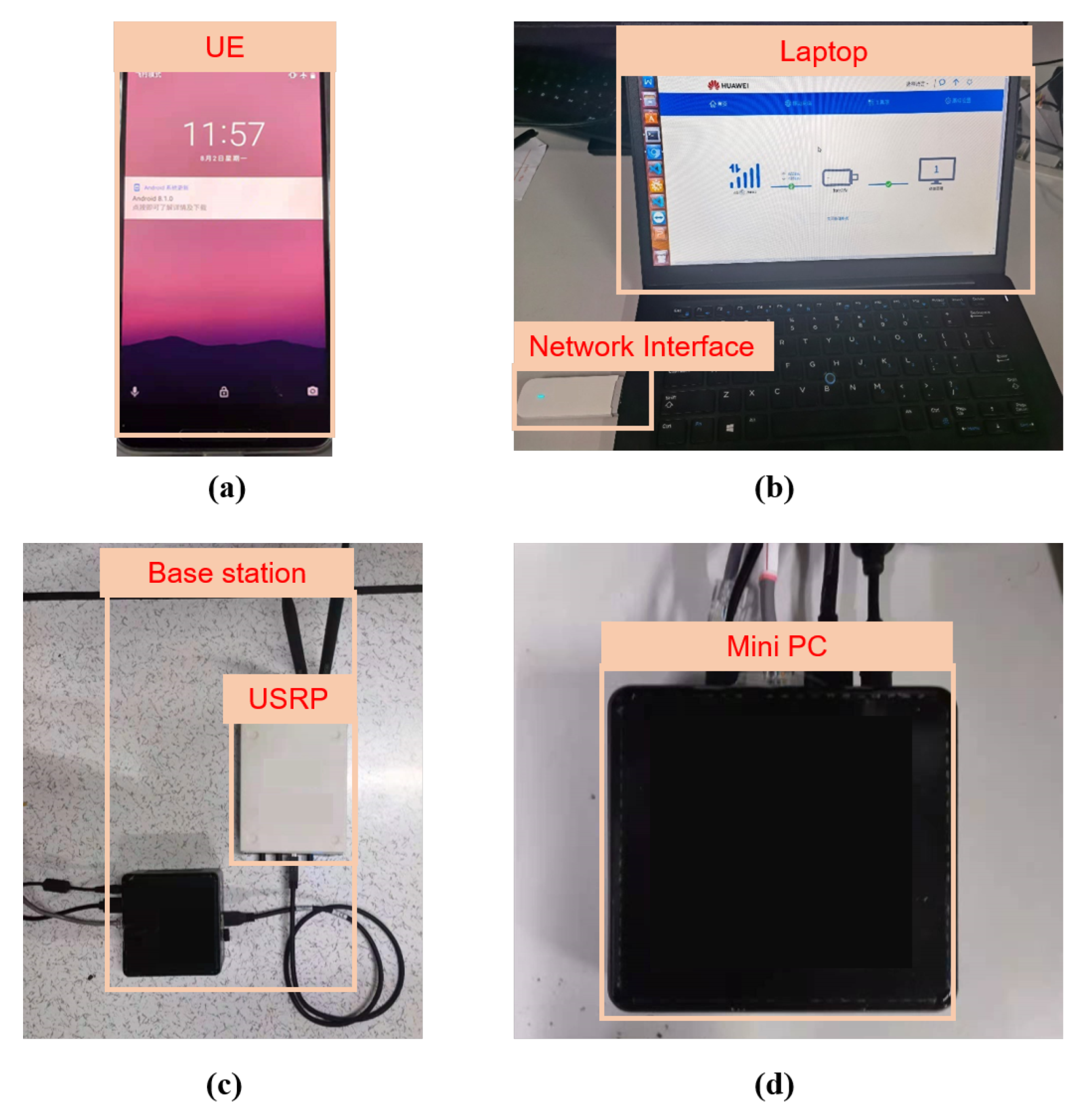
5.2. Prototyping Results

In order to provide more practical insights and verify that our proposed algorithm is also applicable in a practical environment, we collect the interference data on a prototype system as shown in Figure 6, which utilizes the open air interface (OAI) [25] enabled software defined radio to model the network topology as depicted in Figure 1. OAI has complete 5G and LTE protocol stacks, and the protocol parameters during the transmission can be easily collected through the interface to the software FlexRAN [26]. The radio frequency front-end uses the Universal Software Radio Peripheral (USRP) B210 [27], which provides a fully integrated, single-board platform to realize the digital baseband and intermediate frequency parts of the radio communication system. The commercial UE uses the Huawei Nexus 6P with the customized SIM card and the DELL laptop with a SIM card in the Huawei E3372 wireless network interface. The mini PC we used is the Intel NUC8iBEH made in China, which has Intel®i7-8559U CPU, 16GB RAM, and an Ubuntu16.04 operating system. OAI and FlexRAN are both running on it, and each mini PC has a network cable connected to the internet, which can serve the connected UE to access online resources.

In the prototype measurement, we set up a test environment with three BSs, one target UE, and many neighboring UEs as shown in Figure 7. Two neighboring BSs (e.g., B_Ncell and C_Ncell) serve neighboring UEs with real-time video streaming applications, which generates interference to the transmission link between the serving BS (e.g., A_Pcell) and the target UE. Two interference conditions are considered in the prototype evaluation, including single interference source (only B_Ncell is active) and double interference source (B_Ncell and C_Ncell are active). All of them share the same spectrum, and other parameters applied in the prototype evaluation are shown in

Table 3. The parameters of the base station in the prototyping system.

Parameters	Value	Parameters	Value
Frame Type	FDD	TX Antennas Num	1
Downlink Frequency	26.75 MHz	RX Antennas Num	1
Bandwidth	10 MHz	TX Gain	−90 dB
Prefix Type	Normal	RX Gain	125 dB

.

When collecting data, we first connect the neighboring UEs to the corresponding neighboring base station and start the real-time video streaming application. The neighbor base station in work mode is shown in Figure 8. Then, we connect the target UE with the serving cell and start the data collection script to obtain data from the interface of FlexRAN. The data acquisition period is set to 100 milliseconds. In the case of a single interference source, one neighboring base station (e.g., C_Ncell) and the UE connected with it stop working. Under the two kinds of interference conditions, we collected two hours of data, and the data amounts were 72,366 and 73,010, respectively.

In Figure 9, we plot the reward training curves and compare the performance of each baseline. As shown in the figure, the methods based on DQN have converged, and our method has better gain and is much closer to the genie-aided bound. Compared between Figure 4 and Figure 9, we know that the schemes using the DQN method (Baseline 4, ours and genie-aided) have better gain when the measured data of the actual system are used as experimental data. In Figure 10, we plot the statistics of the achievable throughput for different episodes under the data from the prototype system. Our proposed method also has good performance. Compared with the baselines with prediction methods, such as Baseline 1, 2 and 4, our methods have an average throughput gain of 164.4%, 293.0% and 8.0% for the single interference source case, and 354.2%, 592.9% and 19.7%, for the double interference source case, respectively. By comparing with Baseline 3, our proposed method achieves 20.8% and 113.2% average throughput gain for the single and double interference source cases, respectively. We compare the performance loss of each algorithm with the genie-aided method and summarize them in

Table 4. The throughput and performance loss of different methods in the prototyping result.

	Single Interference Source		Double Interference Source
	Throughput	Performance Loss	Throughput	Performance Loss
Baseline 1	61.1	0.668	29.9	0.808
Baseline 2	41.1	0.777	19.6	0.874
Baseline 3	133.7	0.273	63.7	0.592
Baseline 4	149.6	0.188	133.5	0.273
Ours	161.6	0.123	135.8	0.130
Genie-aided	184.1	0	156.0	0

, and we can see that our algorithm has better performance.

6. Conclusions

In this paper, we propose an interference-aware resource-allocation strategy using the channel condition and interference prediction-based scheme for non-cooperative multi-cell transmission. By jointly utilizing the historical channel and interference information, our proposed scheme is able to provide superior average throughput gain over the existing baseline schemes. Through some numerical as well as prototyping results, we show that the proposed method can achieve average throughput gains from 9.7% to 906.0% for the numerical evaluation, and 8% to 592.9% for the prototype evaluation, respectively.

References

1. Hamza, A.S.; Khalifa, S.S.; Hamza, H.S.; Elsayed, K. A Survey on Inter-Cell Interference Coordination Techniques in OFDMA-Based Cellular Networks. IEEE Commun. Surv. Tutor. 2013, 15, 1642–1670. [Google Scholar] [CrossRef]
2. Suo, L.; Li, H.; Zhang, S.; Li, J. Successive Interference Cancellation and Alignment in K-user MIMO Interference Channels with Partial Unidirectional Strong Interference. China Commun. 2022, 19, 118–130. [Google Scholar] [CrossRef]
3. Kim, H.; Kim, J.; Hong, D. Dynamic TDD Systems for 5G and Beyond: A Survey of Cross-Link Interference Mitigation. IEEE Commun. Surv. Tutor. 2020, 22, 2315–2348. [Google Scholar] [CrossRef]
4. Elhattab, M.; Arfaoui, M.A.; Assi, C. A Joint CoMP C-NOMA for Enhanced Cellular System Performance. IEEE Commun. Lett. 2020, 24, 1919–1923. [Google Scholar] [CrossRef]
5. Seifi, N.; Zhang, J.; Heath, R.W.; Svensson, T.; Coldrey, M. Coordinated 3D Beamforming for Interference Management in Cellular Networks. IEEE Trans. Wirel. Commun. 2014, 13, 5396–5410. [Google Scholar] [CrossRef]
6. Qamar, F.; Hindia, M.H.D.N.; Dimyati, K.; Noordin, K.A.; Amiri, I.S. Interference Management Issues for the Future 5G Network: A Review. Telecommun. Syst. 2019, 71, 627–643. [Google Scholar] [CrossRef]
7. Han, S.; Yang, C.; Chen, P. Full Duplex-Assisted Intercell Interference Cancellation in Heterogeneous Networks. IEEE Trans. Commun. 2015, 63, 5218–5234. [Google Scholar] [CrossRef]
8. Yu, Z.; Hou, J. Research on Interference Coordination Optimization Strategy for User Fairness in NOMA Heterogeneous Networks. Electronics 2022, 11, 1700. [Google Scholar] [CrossRef]
9. Evolved Universal Terrestrial Radio Access (E-UTRA) and Evolved Universal Terrestrial Radio Access Network (E-UTRAN); Overall description; Stage 2. TS 36.300, 3GPP. R17. 2022. Available online: https://www.etsi.org/deliver/etsi_ts/136300_136399/136300/17.01.00_60/ts_136300v170100p.pdf (accessed on 12 December 2022).
10. Chan, C.Y.; Chang, G.Y. A Beam-Based eICIC Algorithm. In Proceedings of the 2020 21st Asia-Pacific Network Operations and Management Symposium (APNOMS), Daegu, Republic of Korea, 22–25 September 2020; pp. 421–427. [Google Scholar] [CrossRef]
11. Maruta, K. Imperfect CSI Muting With Time-Domain Thresholding for Cooperative Intercell Interference Cancellation. IEEE Syst. J. 2022, 16, 1147–1157. [Google Scholar] [CrossRef]
12. Jiang, S.; Chang, Y.; Fukawa, K. Distributed Inter-cell Interference Coordination for Small Cell Wireless Communications: A Multi-Agent Deep Q-Learning Approach. In Proceedings of the 2020 International Conference on Computer, Information and Telecommunication Systems (CITS), Hangzhou, China, 5–7 October 2020; pp. 1–5. [Google Scholar] [CrossRef]
13. Zheng, J.; Gao, L.; Zhang, H.; Niyato, D.; Ren, J.; Wang, H.; Guo, H.; Wang, Z. eICIC Configuration of Downlink and Uplink Decoupling With SWIPT in 5G Dense IoT HetNets. IEEE Trans. Wirel. Commun. 2021, 20, 8274–8287. [Google Scholar] [CrossRef]
14. Ye, Y.; Shi, L.; Chu, X.; Hu, R.Q.; Lu, G. Resource Allocation in Backscatter-Assisted Wireless Powered MEC Networks with Limited MEC Computation Capacity. IEEE Trans. Wirel. Commun. 2022, 21, 10678–10694. [Google Scholar] [CrossRef]
15. Moosavi, N.; Sinaie, M.; Azmi, P.; Lin, P.H.; Jorswieck, E. Cross Layer Resource Allocation in H-CRAN with Spectrum and Energy Cooperation. IEEE Trans. Mob. Comput. 2021, 22, 145–158. [Google Scholar] [CrossRef]
16. Jarinová, D. Fading Channel Prediction by Higher-Order Markov Model. In Proceedings of the 2020 New Trends in Signal Processing (NTSP), Demanovska Dolina, Slovakia, 14–16 October 2020; pp. 1–4. [Google Scholar] [CrossRef]
17. Zhao, G.; Li, Y.; Xu, C.; Han, Z.; Xing, Y.; Yu, S. Joint Power Control and Channel Allocation for Interference Mitigation Based on Reinforcement Learning. IEEE Access 2019, 7, 177254–177265. [Google Scholar] [CrossRef]
18. Sheng, M.; Wen, J.; Li, J.; Liang, B.; Wang, X. Performance Analysis of Heterogeneous Cellular Networks With HARQ Under Correlated Interference. IEEE Trans. Wirel. Commun. 2017, 16, 8377–8389. [Google Scholar] [CrossRef]
19. He, Y.; Zhang, Z.; Yu, F.R.; Zhao, N.; Yin, H.; Leung, V.C.M.; Zhang, Y. Deep-Reinforcement-Learning-Based Optimization for Cache-Enabled Opportunistic Interference Alignment Wireless Networks. IEEE Trans. Veh. Technol. 2017, 66, 10433–10445. [Google Scholar] [CrossRef]
20. Evolved Universal Terrestrial Radio Access (E-UTRA); Physical Layer Procedures. TS 36.213, 3GPP. R17. 2022. Available online: https://www.etsi.org/deliver/etsi_ts/136200_136299/136213/17.01.00_60/ts_136213v170100p.pdf (accessed on 12 December 2022).
21. Kim, H.; Kim, S.; Lee, H.; Jang, C.; Choi, Y.; Choi, J. Massive MIMO Channel Prediction: Kalman Filtering vs. Machine Learning. IEEE Trans. Commun. 2021, 69, 518–528. [Google Scholar] [CrossRef]
22. Li, Q.; Li, R.; Ji, K.; Dai, W. Kalman Filter and Its Application. In Proceedings of the 2015 8th International Conference on Intelligent Networks and Intelligent Systems (ICINIS), Tianjin, China, 1–3 November 2015; pp. 74–77. [Google Scholar] [CrossRef]
23. Liu, L.; Cai, L.; Ma, L.; Qiao, G. Channel State Information Prediction for Adaptive Underwater Acoustic Downlink OFDMA System: Deep Neural Networks Based Approach. IEEE Trans. Veh. Technol. 2021, 70, 9063–9076. [Google Scholar] [CrossRef]
24. Yu, Y.; Liew, S.C.; Wang, T. Non-Uniform Time-Step Deep Q-Network for Carrier-Sense Multiple Access in Heterogeneous Wireless Networks. IEEE Trans. Mob. Comput. 2021, 20, 2848–2861. [Google Scholar] [CrossRef]
25. Oai /openairinterface5G · GitLab. Available online: https://gitlab.eurecom.fr/oai/openairinterface5g (accessed on 12 December 2022).
26. Foukas, X.; Nikaein, N.; Kassem, M.M.; Marina, M.K.; Kontovasilis, K. FlexRAN: A Flexible and Programmable Platform for Software-Defined Radio Access Networks. In Proceedings of the 12th International on Conference on Emerging Networking EXperiments and Technologies, Irvine, CA, USA, 12–15 December 2016; ACM: New York, NY, USA, 2016; pp. 427–441. [Google Scholar] [CrossRef]
27. Brand, a National Instruments, E.R. USRP B210 USB Software Defined Radio (SDR). Available online: https://www.ettus.com/all-products/ub210-kit/ (accessed on 12 December 2022).
Figure 1. Subfigure (a) shows the inter-cell interference between UE and base stations in the multi-cell scenario. The hexagon is the transmission range of the base station signal. Subfigure (b) shows the inter-cell interference scenario abstracted from A, where UE1 has one interference cell and UE2 has two interference cells.
Electronics 12 00868 g001
Figure 2. Every time slot downlink data transmit process flow chart.
Electronics 12 00868 g002
Figure 3. The slide window used in the dataset generation (e.g., W t = 3 and W f = 3 ) and the LSTM prediction network model.
Electronics 12 00868 g003
Figure 4. Reward convergence of the DQN method for the numerical result and the comparison of reward among different methods. The top is for single interference source, the bottom is for double interference source.
Electronics 12 00868 g004
Figure 5. The box plot of total throughput for 100 time slots in each training episode under the simulation data.
Electronics 12 00868 g005
Figure 6. The pictures of the prototype system. (a,b) are two types of commercial UE, (c) is the software-defined base station with frequency front-end USRP, and (d) is the mini PC.
Electronics 12 00868 g006
Figure 7. The map of the indoor test site.
Electronics 12 00868 g007
Figure 8. The neighbor base station is working. The UEs are playing the online video to occupy the bandwidth. The monitor shows the running status of the base station.
Electronics 12 00868 g008
Figure 9. Reward convergence of the DQN method for the prototyping result and the comparison of reward among different methods. The top is for single interference source, the bottom is for double interference source.
Electronics 12 00868 g009
Figure 10. The box plot of total throughput for 100 time slots in each training episode under the prototyping data.
Electronics 12 00868 g010