Optimized and Efficient Color Prediction Algorithms Using Mask R-CNN

Abstract

Color cognizant capability has a significant impact in service robots for object detection based on color, traffic signal interpretation for autonomous vehicles, etc. Conventional clustering algorithms such as K-means and mean shift can be used for predicting the dominant color of an image by mapping the pixels from RGB to HSV and clustering them based on HSV values, thereby picking the cluster with the most pixels as the dominant color of the image, but these approaches are not solely dedicated to the same outcome. This research’s goal is to introduce novel techniques for predicting the dominant color of objects in images, as well as pixel extraction concepts, which allow these algorithms to be more time and efficiency optimized. This investigation appraises propriety of integrating object detection and color prediction algorithms. We introduce a dominant color prediction color map model and two new algorithms: average windowing and pixel skip. To predict objects in an image prior to color prediction, we combined the Mask R-CNN framework with our proposed techniques. Verification of our approach is done by creating a benchmark dataset of 200 images and comparing color predicted by algorithms with actual color. The accuracy and runtime of existing techniques are compared with those of the proposed algorithms to prove the superiority of our algorithms. The viability of the proposed algorithms was demonstrated by scores of 95.4% accuracy and color prediction time of 9.2 s for the PXS algorithm and corresponding values of 93.6% and 6.5 s for the AVW algorithm.

1. Introduction

Proliferating deployment of robotics and autonomous applications in diverse aspects of everyday life in recent times has aroused keen interest of researchers in the domain of detection and identification of objects. Such attributes outfit robots with a capability to mimic human behavior. Deep learning techniques have become popular these days for implementing object detection. Some of the applications of deep learning techniques apart from object detection include facial recognition [1,2], gesture recognition [3,4], health care [5,6], image enhancement [7], etc. Object detection assumes a dominant role in the field of automation, harmonized with increased precision and simplification of work. Object detection gadgets are conspicuous in video surveillance, security cameras, and self-driving systems [8]. Object detection models introduced in the past decade include region-based convolutional neural networks (R-CNN), Fast R-CNN, you only look once (YOLO), and Mask R-CNN [9]. The deployed models are enhanced versions of primitive CNN models. CNN models are also widely used for object recognition and classification [7]. YOLO and R-CNN are esteemed for their accurate detection of objects [10,11]. The pretrained model employed in Mask R-CNN is used for detecting objects in the input image and as an input for our proposed algorithms that are discussed in the later sections. Dominant color extraction from an image is a frequently used technique in applications such as image segmentation, medical image analysis, image retrieval, and image mixing [12]. Although many algorithms are available for detection of the dominant color of an object, they are based on clustering techniques that are deficient in time complexity or in accuracy in color prediction. Hence, we have introduced two algorithms based on new techniques for predicting the dominant color of an object in the image. The two algorithms, AVW and PXS, use averaging and skipping techniques respectively, to select pixels from an input image. These algorithms have huge importance in terms of time as most of the pixels in the image are eliminated while predicting color (which will be discussed in the later sections) to save time without compromising on accuracy. The DCPCM model predicts the color of all input pixels given by the proposed algorithms.

Initially, YOLO was selected for object detection, as it is one of the fastest object detection models [10]. But YOLO does not provide a mask along with the bounding box for the detected object, which results in reduced accuracy, as some background pixels inside the bounding box that are not part of the object may contribute to the color prediction and may disrupt the final color predicted. Isolation of the pixels contributing to the background of the object, enclosed within the masked portion of AVW and PXS algorithms, facilitate increased accuracy in the predictions of the (dominant) color of an object. Concurrently, the runtime for predicting the object’s color is significantly diminished as the number of pixels considered for prediction gets reduced. Unlike other object detection algorithms, Mask R-CNN, outfitted with a segmentation mask for each object detected, is preferred for integration with our proposed algorithms purposes. Mask R-CNN has also been found to be more efficient in detecting the type of vehicles, for video surveillance and self-driving systems [13], where color prediction of objects can be an added advantage. Nevertheless, the AVW and PXS algorithms are flexible enough to be unified with any application that requires color prediction. The canny edge detection approach is used to identify the nonuniformity percentage for every object detected in an image. This technique detects a wide variety of edges in images by noise suppression [14], yet it is applicable only to grayscale images, returning a binary matrix of dimensions, stating whether the respective pixel contributes to an edge or not. Average pixel width (APW) is the average of the entire binary matrix. APW is more likely to give the percentage of nonuniformity in an image [15], which is used to model the algorithms propounded in Section 5.

HSV is a color model of cylindrical shape that transforms the red green blue (RGB) color model into easily comprehensible dimensions [16]. Hue determines the angle of color on the HSV and RGB circles. Saturation represents the amount of color being used, and value represents the level of brightness of the respective color. Supervened by its balanced color perception capability, HSV color space is DCPCM model [17]. Elaborated in Section 3, the entire HSV color space, marshalled in the proposed model, is mapped into 15 basic color classes to provide a better understanding and readability of the DCPCM’s output. The existing techniques of color prediction are based on clustering. Clustering refers to the process of grouping the available data points (pixels in the context of color prediction) into different clusters based on their similarity with certain parameters such as color, features, etc. Clustering is commonly applied to predict the dominant color of an image [18,19]; K-means, mean shift, and fuzzy C-means are a few popular clustering models [20]. Hence, this calls for a simple dedicated algorithm for prediction of the dominant color in an image. These clustering algorithms excel in various machine learning applications [21,22,23,24,25,26].

An edge detector scheme, adaptable for real-time applications, is presented in [27]; the results presented in [27] show that the proposed method of edge detection outperforms other existing methods in terms of accuracy. A model that discerns humans from the background in a video and identifies the actions performed by him or her was proposed in [28,29]. It introduced a scheme to discriminate between red and black grapes using image detection and color prediction schemes. A hierarchical interactive refinement network, which facilitates effective preservation of edge structures while detecting salient objects, was illustrated in [30]. An efficient method that exploited mean-shift clustering, was elucidated in [31], for the discovery of common visual patterns (CVPs) between two images. An enhanced version of Mask R-CNN for the detection of cucumber in greenhouses, was demonstrated in [32]. Recently [33], reports were published on an application of HSV combined with K-means clustering in the detection of food spoilage. A comparative analysis of the execution times between the software implementation and register-transfer level (RTL) design of the Sobel edge detection algorithm was presented in [34]. A scheme for identification of an object, based on recognition of its color and contour, through digital image processing techniques was presented in [35]. A technique for the segregation of objects in an image based on their color, alleviates the complexities of boundary detection [36]. A hybrid method that extracts the spatial information and color for identification of the moving objects in a video was presented [37].

We summarize below the limitations of the clustering algorithms in color prediction.

• The clustering algorithms are not exclusively designed for color prediction. They also excel in various machine learning applications;
• The K-value is not easy to predict in K-means algorithm, which does not go well with global clusters. In addition, the time complexity of K-means increases if the datasets are bigger;
• Mini batch K-means algorithm has lower accuracy than K-means;
• Time complexity is a major disadvantage in mean shift algorithm;
• GMM takes more time to converge and hence slower than K-means;
• Fuzzy C-means requires greater number of iterations for better results.

The purpose of this study is to address the limitations of clustering algorithms in color prediction. We propose a model that is exclusively used for color prediction and not for any other purpose. In addition, we propose two new algorithms that can extract dominant colors accurately in less time. In view of this, a dominant color prediction color map (DCPCM) model and two new algorithms, average windowing (AVW) and pixel skip (PXS), are presented in this work. To predict the color of the object in an image, we need to detect the object first. For this purpose, we integrate the Mask R-CNN algorithm with our proposed techniques to predict the objects in the image prior to color prediction. Rather than considering all the pixels of the object, the AVW algorithm takes the average of the section/window of the pixels from the image at a time and repeats the averaging for the entire object in the image. Because of this, the overall time for color prediction decreases. At the same time, it maintains good accuracy because the window size is chosen according to the uniformity of the color in the object. On the other hand, the PXS algorithm skips the pixels selectively based on the uniformity of the color in the object. This results in less time for color prediction without compromising much accuracy.

The main contributions of this research work are listed below:

• A color prediction model called DCPCM that is exclusively designed by uniquely categorizing HSV domain values into 15 different color classes, to be used only for color prediction and not for any other purpose. The main aim of the given model is to reduce the color spectrum into 15 commonly used colors, thereby reducing the complexity and the runtime.
• Two new algorithms called AVW and PXS to selectively extract pixels from an image, using precomputed formulae, thereby reducing the runtime and maintaining the accuracy;
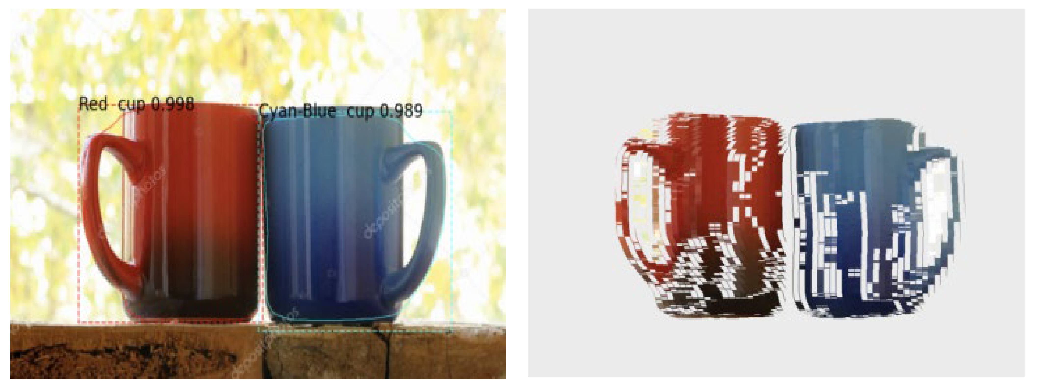
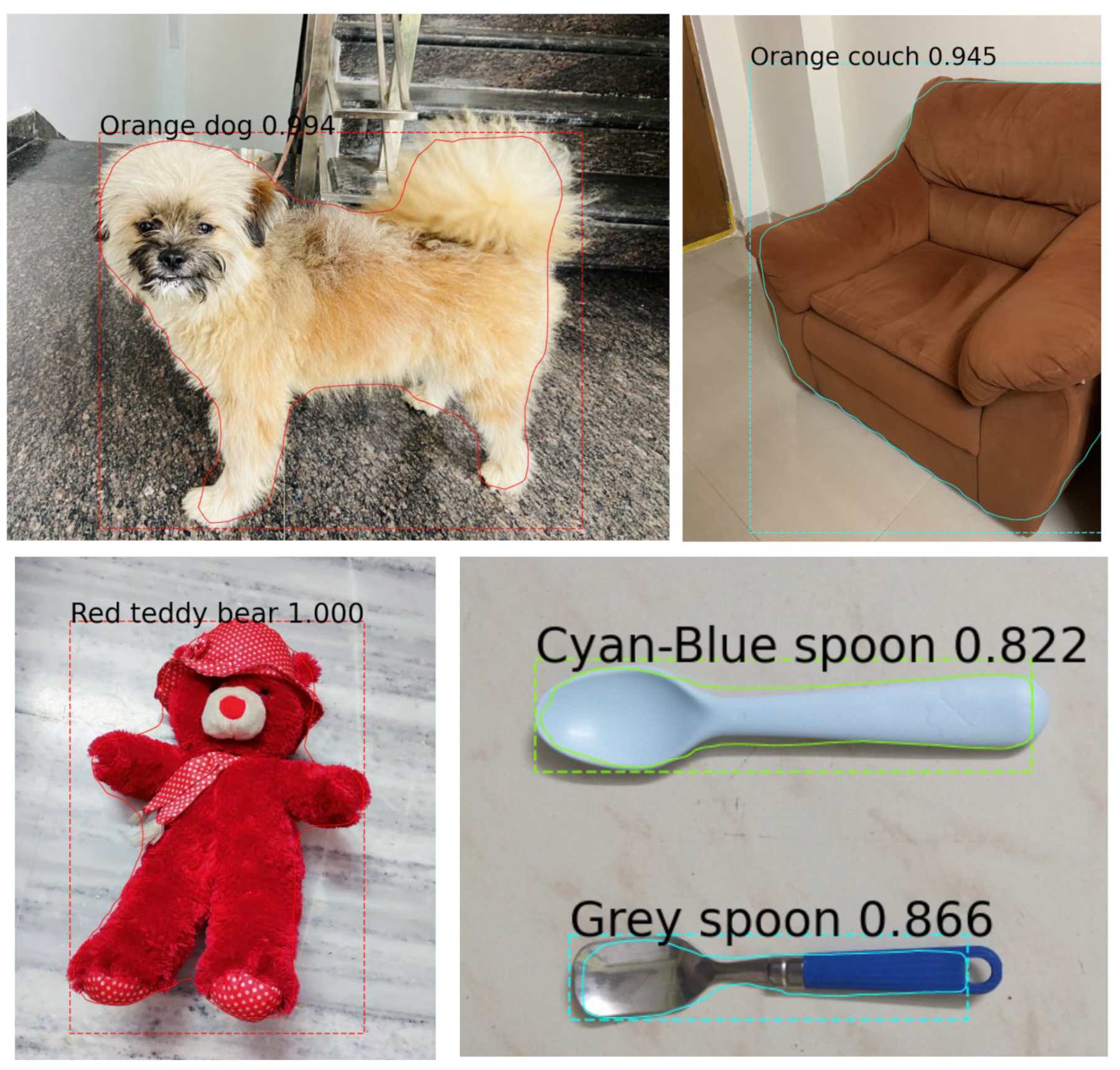
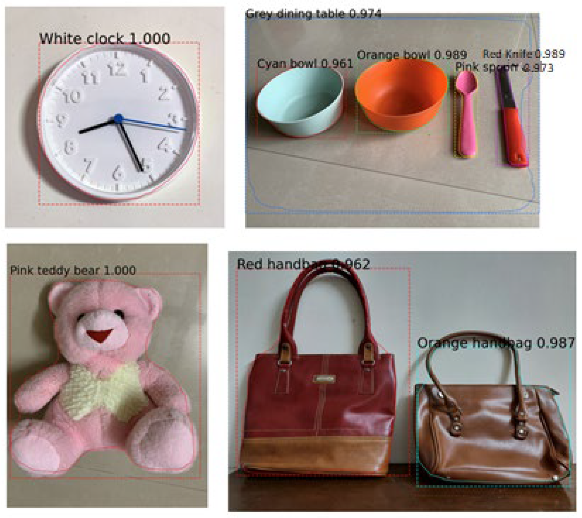
• Integration of Mask-RCNN algorithm with the proposed techniques for identifying the objects in the image prior to pixel extraction and dominant color prediction;
• Creation of benchmark data set with 200 images of single object, multi-object, uniformly colored, multicolored and of various sizes, to test the proposed algorithms and compare them with the existing clustering techniques stated above.

The rest of the paper is organized as follows. Section 2 summarizes the entire working of the system using an architecture diagram. The technical aspects of the work start from Section 3, by presenting the DCPCM model, which is then followed by Section 4, describing AVW and PXS algorithms in a detailed manner. Section 5 presents the experimental results followed by Section 6, which deals with proving the supremacy of AVW and PXS over the existing techniques for color prediction. Section 7 provides discussion on the results and concludes the work.

2. System Architecture

The system architecture diagram shown in Figure 1 presents the workflow of the proposed AVW and PXS algorithms that predict the object class using the Mask R-CNN framework, along with its color property. Consider an input image that contains two bowls, a knife, and a spoon, as shown in Figure 1. When the proposed algorithm AVW/PXS is executed, this image is assigned and stored in the form of a matrix. Subsequently, the matrix triggers the object detection function that predicts the objects along with other parameters like bounding boxes, and mask color. If objects are detected in the image, then the proposed algorithms store the location of objects, i.e., its bounding box coordinates, along with its masked portion. After prediction, the masked pixels are filtered out and sent as an input to the algorithm block, i.e., AVW or PXS. Simultaneously, preprocessing happens for the given object to calculate a few parameters required for the algorithms using canny edge detection.

The DCPCM model is integrated with both AVW and PXS algorithms that map pixels to their respective color class among the fifteen predetermined colors. After the execution of AVW/PXS, the output is displayed in a separate window that contains the objects surrounded by their bounding boxes, the object’s class, and its dominant color. This process repeats for every object detected by the Mask R-CNN framework. If no objects are found in the image, then the algorithm simply displays “No object detected” and the same input image is shown as the output in the Jupyter notebook. The DCPCM model skips the color prediction step if the object detected is a person to avoid controversies as the model can predict the costume color as the color of a person. This architecture is helpful in classification of similar objects based on color that have wide applications in the service robot sector.

3. Dominant Color Prediction Color Map (DCPCM) Model

There are many shades of different colors available in each color space. Some of the color spaces are HSV, cyan magenta yellow key (CMYK), and RGB. Generally exposed to various color shades or trained, human beings are capable of predicting the color of an object merely by a glance at an object, unlike a machine that perceives an image in the form of a pixel constituted of three channels: red, green and blue. In order to predict the dominant color of an object, algorithms are required to iterate through all the pixels of an object image, and maintain counts of the various colors, ensuing the prediction of the dominant color. In order to generalize the HSV color space, all the available color shades are classified into 15 color classes: red, green, blue, yellow, cyan, magenta, orange, yellow-green, green-cyan, cyan-blue, violet, pink, gray, white, and black. Fifteen colors are chosen because they are the ones most widely used that include primary, secondary, tertiary, and neutral colors. HSV values range from [0,360], [0,100], [0,100]. Hence, the range of each pixel is 9 × 7 × 7 bits. The DCPCM model extracts each pixel in an object and maps it into one of the 15 predetermined color classes.

The saturation (S) and value (V) parameters of the HSV color model are split into three ranges—low, medium, and high. These ranges are shown in Equations (1) and (2).

$$S_1\left(S\right)= \left\{\begin{array}{c}Low if Sϵ\left[0,13\right]\\ Medium if Sϵ\left[14,50\right]\\ High if Sϵ\left[51,100\right]\end{array}\right.\hspace{1em}\mathrm{Ranges} \mathrm{of} \text{“}S\text{”} \mathrm{parameter}$$

(1)

S₁ is the name of the range in which “S” belongs.

$$V_1\left(V\right)= \left\{\begin{array}{c} Low if Vϵ\left[0,15\right]\\ Medium if Vϵ\left[16,75\right]\\ High if Vϵ\left[76,100\right]\end{array}\right.\hspace{1em}\mathrm{Ranges} \mathrm{of} \text{“}V\text{”} \mathrm{parameter}$$

(2)

V₁ is the name of the range in which “V” belongs.

The main objective of the DCPCM model is to predict colors for various combinations of the low, medium, and high ranges. The nine combinations available from different ranges are shown in

Table 1. Combinations of “S” and “V” parameters.

Saturation (S1)	Value (V1)	Color
Low	Low	Black
Low	Medium	Gray
Low	High	White
Medium	Low	Black
Medium	Medium	Only Tertiary colors (3)
Medium	High	Secondary and Tertiary colors (4)
High	Low	Black
High	Medium	Primary and Tertiary colors (5)
High	High	All colors (6)

. Among these nine combinations of “S” and “V” parameters, for five combinations the color is treated as black, gray, or white, whereas the colors for the remaining four combinations are based on values of the “H” parameter. These four combinations are shown in Equations (3)–(6).

$$\mathit{Color}=\left\{\begin{array}{cc}\mathit{Orange}& \mathit{if}\mathit{H}\left({}^{\circ }\right)ϵ[15,45]\\ \mathit{Yellow}-\mathit{Green}& \mathit{if}\mathit{H}\left({}^{\circ }\right)ϵ[46,110]\\ \mathit{Green}-\mathit{Cyan}& \mathit{if}\mathit{H}\left({}^{\circ }\right)ϵ[111,175]\\ \mathit{Cyan}-\mathit{Blue}& \mathit{if}\mathit{H}\left({}^{\circ }\right)ϵ[176,240]\\ \mathit{Violet}& \mathit{if}\mathit{H}\left({}^{\circ }\right)ϵ[241,310]\\ \mathit{Pink}& \mathit{otherwise}\end{array}\right.$$

(3)

Predictions for the combination S = “medium” and V = “medium”.

$$\mathit{Color}=\left\{\begin{array}{cc}\mathit{Orange}& \mathit{if}\mathit{H}\left({}^{\circ }\right)ϵ[15,40]\\ \mathit{Yellow}& \mathit{if}\mathit{H}\left({}^{\circ }\right)ϵ[41,60]\\ \mathit{Yellow}-\mathit{Green}& \mathit{if}\mathit{H}\left({}^{\circ }\right)ϵ[61,110]\\ \mathit{Green}-\mathit{Cyan}& \mathit{if}\mathit{H}\left({}^{\circ }\right)ϵ[111,150]\\ \mathit{Cyan}& \mathit{if}\mathit{H}\left({}^{\circ }\right)ϵ[151,190]\\ \mathit{Cyan}-\mathit{Blue}& \mathit{if}\mathit{H}\left({}^{\circ }\right)ϵ[191,225]\\ \mathit{Violet}& \mathit{if}\mathit{H}\left({}^{\circ }\right)ϵ[226,280]\\ \mathit{Magenta}& \mathit{if}\mathit{H}\left({}^{\circ }\right)ϵ[281,330]\\ \mathit{Pink}& \mathit{otherwise}\end{array}\right.$$

(4)

Predictions for the combination S = “medium” and V = “high”.

$$\mathit{Color}=\left\{\begin{array}{cc}\mathit{Red}& \mathit{if}\left(\mathit{H}\left({}^{\circ }\right)ϵ[0,10]\mathit{or}\mathit{H}\left({}^{\circ }\right)ϵ[331,360]\right)\\ \mathit{Orange}& \mathit{if}\mathit{H}\left({}^{\circ }\right)ϵ[11,50]\\ \mathit{Yellow}-\mathit{Green}& \mathit{if}\mathit{H}\left({}^{\circ }\right)ϵ[51,75]\\ \mathit{Green}& \mathit{if}\mathit{H}\left({}^{\circ }\right)ϵ[76,135]\\ \mathit{Green}-\mathit{Cyan}& \mathit{if}\mathit{H}\left({}^{\circ }\right)ϵ[136,165]\\ \mathit{Cyan}-\mathit{Blue}& \mathit{if}\mathit{H}\left({}^{\circ }\right)ϵ[166,210]\\ \mathit{Blue}& \mathit{if}\mathit{H}\left({}^{\circ }\right)ϵ[211,265]\\ \mathit{Violet}& \mathit{if}\mathit{H}\left({}^{\circ }\right)ϵ[266,295]\\ \mathit{Pink}& \mathit{otherwise}\end{array}\right.$$

(5)

Predictions for the combination S = “high” and V = “medium”.

$$S_1 \left(S\right)=\left\{\begin{array}{c}Low if Sϵ\left[0,13\right]\\ Medium if Sϵ\left[14,50\right]\\ High if Sϵ\left[51,100\right]\end{array}\right.\hspace{1em}\mathrm{Ranges} \mathrm{of} \text{“}S\text{”} \mathrm{parameter}$$

(6)

Predictions for the combination S = “high” and V = “high”.

4. AVW and PXS Algorithms

This section presents the terminologies used in the proposed algorithm first, followed by relevant details of the AVW and PXS algorithms. The all-pixel approach for predicting the dominant color of the object using the DCPCM model is discussed first. Later, we move on to present the AVW algorithm and the PXS algorithm.

A detailed list of symbols used for modeling AVW and PXS is given in

Table 2. Symbols used for modeling AVW and PXS.

Saturation (S1)	Value (V1)
M	Length of the Original Image.
N	Width of the Original Image.
[Mc]1 × 3	This represents the Masked Color of the Original Image. This notation implies that Im is a matrix of dimension 1 × 3 (since it has 3 channels i.e., R, G, B).
[Io]m × n	Original Image Data. This notation implies that Io is a matrix of size m × n.
[Im]m × n	Masked Image Data. This notation implies that Im is a matrix of size m × n.
R	Variable that iterates through rows of [Io] and [Im].
C	Variable that iterates through columns of [Io] and [Im].
Dc	Dominant color of the image.
[K]m × n × 15	Matrix representing the result of DCPCM model for the respective pixel. The number 15 in the notation represents the predetermined colors.
T	Length of list containing masked pixels.

.

4.1. Preprocessing Required for AVW and PXS Algorithms

This section lists the terminologies used while defining the algorithms AVW and PXS. The terminologies and definitions presented here are common to both AVW and PXS. Let (y1, x1), and (y2, x2) be the top-left and bottom-right coordinates of the bounding box for an object predicted in the input image after the image passes through the Mask R-CNN block shown in Figure 1.

Let the object currently predicted be referred to as the current object.

• Masked Color, represents the RGB values of the mask chosen by Mask R-CNN, for the current object;
• Masked_Image, is the image obtained after application of the respective mask, Mask R-CNN, to the Original_Image;
• OriginalImageData, is the matrix that stores the pixel representations of the Original_Image in terms of RGB channels.
• MaskImageData, is the matrix that stores the pixel representations of the Masked_Image in terms of RGB channels.
• Color_Set, is an array that stores the predetermined colors, by allocations of an index to each of the 15 colors and represented as [C_SET]_1*15. This notation implies that the Color_Set, is a 1*15 matrix i.e., a 1-D array that stores all the 15 colors. [C_SET] = [“Red”, “Orange”, “Yellow”, “Yellow-Green”, “Green”, “Green-Cyan”, “Cyan”, “Cyan-Blue”, “Blue”, “Violet”, “Magenta”, “Black”, “Pink”, “White”, “Gray”].
• R2H (r, g, b), represents a function that takes in the RGB values of a pixel and returns the respective HSV value.
• C_P (h, s, v), represents a function that takes in the HSV values of a pixel and returns the respective color class. This pertains to implementation of the DCPCM model, discussed in the previous section.
• [G_scale], is the grayscale representation of an original image [I_o].
• Edgecanny (A_m), represents the canny edge detector function, discussed previously in Section 1. It gives us the APW i.e., average number of pixels contributing to edges in the given matrix A_m, where A_m is the resultant output, after the [G_scale] passes through the edge_filter.
• Edge_filter filters out the pixels contributing to the unmasked portion of the current object. Since the uniformity is based on the edges, the pixel contributing to the unmasked portion inside the bounding box is converted to “white”. This operation will exclude the unmasked portion for uniformity prediction while maintaining the null spaces in the input matrix.

4.2. All-Pixel Approach

Let [A]_1*15 be the 1-D array where each index corresponds to the respective color class and [K] be the matrix representing the result of the DCPCM model for the respective pixel. The steps listed below are preceded by the Mask R-CNN block presented in the system architecture in Figure 1. The steps given below are followed for every object detected in the input image.

Step-1:

Initialize array A to zero.

Step-2:

Iterate through the current_object and increment the respective color of the pixel in [A], if the pixel is inside the bounding box of the current_object and the respective pixel of the masked image is equal to the Masked_Color.

Equations (7) and (8), show a mathematical representation of [A] and [K] for the all-pixel approach. At this stage, the pixel value should be converted from RGB to HSV color space, using R2H (r, g, b).

$$\left[A\right]={\displaystyle \sum }_{r=y1}^{y2}{\displaystyle \sum }_{c=x1}^{x2}K\left[r\right]\left[c\right] \mathrm{if} I_m\left[\mathrm{r}\right]\left[\mathrm{c}\right]=\left[M_c\right].$$

(7)

$$K\left[r\right]\left[c\right]\left[i\right]=\left\{\begin{array}{c}1,C_{SET\left[i\right]}=C\_P\left(h,s,v\right)\\ 0,C_{SET\left[i\right]}\ne C\_P\left(h,s,v\right)\end{array}, \right. \forall i ϵ \left[0,15\right), where h, s, v=R2H\left(I_o\left[r\right]\left[c\right]\right).$$

(8)

Step-3:

Iterate through [A] and find the color with the maximum count which gives us the D_c (dominant color) of the image. Equation (9), represents the mathematical form of Step-3.

$$D_c=C_{SET}\left[i\right], where A\left[i\right]>A\left[j\right], \forall \left(\left(j ϵ \left[0,15\right)\right) \bigcap \left(j!=i\right)\right).$$

(9)

The time complexity of all-pixel approach is O (m × n), where m and n are the width and height of the given object, while the space complexity is O (m × n × 15).

4.3. Average Windowing (AVW) Algorithm

The AVW algorithm decreases the time of the all-pixel approach discussed in Section 4.2 to a greater extent. A window of size “f” is used for implementation of this algorithm. This window slides through the pixels and predicts the average of the RGB channels, at each stop. If the window size is too high, the average of the pixel values may get disrupted and the prediction of dominant color may tend to lose accuracy, whereas if the window size is too small, the run time does not vary much compared to the all-pixel approach. Hence, the value of “f” should be chosen precisely. The concept of uniformity is used to predict “f” that is discussed later in Section 4.3.1. The value of f can vary according to the uniformity factor of the image i.e., the value of “f” increases with an increase in the uniformity factor and vice versa. This algorithm reduces the time complexity to O(T/f) where T is the list of pixels in masked portion of the object and “f” is the window size, but the space complexity remains the same i.e., O(m × n × 15).

A detailed explanation of the AVW algorithm is presented below. The steps listed are preceded by the Mask R-CNN block presented in the system architecture in Figure 1. The steps given below are followed for every object detected in the input image.

Step-1:

Initialize [A] to zero.

Step-2:

Convert the input image into grayscale and store the data into [Gscale].

Step-3:

Iterate through the image and store the pixels from the OriginalImageData that contribute to the masked portion of the MaskedImageData and are inside the bounding box coordinates of the current_object in a list (L) represented in Equation (10).

$$\left[L\right]=I_o\left[r\right]\left[c\right]if I_m\left[r\right]\left[c\right]=\left[Mc\right],\forall \left\{r ϵ W, y_1<=r<=y_2\right\}\& \{c ϵ W,x_1<=r<=x_2\}.$$

(10)

Step-4:

Perform edge detection and predict “f” (Detailed in Section 4.3.1).

Step-5:

Iterate through the list and compute the average of the pixels in each window and increment the respective count in [A]. The mathematical representation of [A], and the result array [K], for AVW are shown in Equations (11) and (12). The representation of average of the HSV values for a particular window is shown in Equation (13).

$$\left[A\right]={\displaystyle \sum }_{\mathrm{r}=\mathrm{y}1}^{\mathrm{y}2}{\displaystyle \sum }_{\mathrm{c}=\mathrm{x}1}^{\mathrm{x}2}\left[K\right]{ \mathrm{if} \mathrm{I}}_{\mathrm{m}}\left[\mathrm{r}\right]\left[\mathrm{c}\right]=\left[M_c\right].$$

(11)

$$K\left[r\right]\left[c\right]\left[i\right]=\left\{\begin{array}{c}1,C_{SET\left[i\right]}=C\_P\left(h,s,v\right)\\ 0,C_{SET\left[i\right]}\ne C\_P\left(h,s,v\right)\end{array},\forall \mathrm{i} ϵ\left[0,15\right).\right.$$

(12)

$$\left[h, s, v\right]=[ \left(\frac{1}{f}\right)\ast {\displaystyle \sum }_{i=j}^{j+f}R2H\left(L\left[i\right]\right)]; j=n\ast f, n \left[0,\left(\frac{T}{f}\right)\right).$$

(13)

Step-6:

Iterate through [A], and find the color with the maximum count, equivalent to the D_c (dominant color) of the image. The extraction of dominant color from the Color-set, is represented in Equation (14).

$${\mathrm{D}}_{\mathrm{c}}=C_{SET}\left[i\right], where A\left[i\right]>A\left[j\right],\hspace{1em} \forall \left(\left(j ϵ \left[0,15\right)\right) \bigcap \left(j!=i\right)\right).$$

(14)

4.3.1. Predicting Window Size (“f”)

Initially, the input image is converted into a grayscale image and stored in [G_scale] array. For each object predicted, the respective bounding box from the image is considered and the unmasked pixels are changed to the same color (i.e., white) so that they do not contribute to the nonuniformity of color in the image. This modified array is sent as an input for the edge detection algorithm. This gives an APW value (refer point-9 in Section 4.1) which is used for predicting “f”. APW of the current_object is more likely to predict the uniformity of an object. If APW is 0, the object is 100% uniform with respect to color. The object is considered as 100% nonuniform with respect to color if the APW is 100.

Let “k” be the number of pixels contributing to edges.

$$k=\frac{APW}{100}\times T.$$

(15)

Let us assume that the k-pixels are uniformly divided in the object (average case). If we consider that 1 window has 1 pixel contributing to edge (assuming that 1 value does not disrupt the average value), then, $f=T/\mathrm{k}$.

According to Equation (15), $f=T\times \frac{100}{APW\times T}$, which on simplification yields Equation (16).

$$f=\frac{100}{APW}.$$

(16)

4.3.2. Pseudo Code of AVW

The pseudo code for the AVW function is shown below. It takes in the list (L) containing the masked pixels, along with the window size “f” and returns the array A, which contains the count of each color class for the input pixels.

AVW (L,f):   //L is the list containing the extracted pixels of the object and “f” is the window size j = 0 while “j” < length (L) var h, s, v <- (0,0,0)   //Defining variables h, s and v. for every “f” pixels. //Loop runs “f” times h, s, v <- (h + L[j][0], s + L[j][1], v + L[j][2]) increment “j” end for //At this point, h, s, and v variables contains sum of the current “f” pixel values. var h_avg,s_avg,v_avg <- (avg(h),avg(s),avg(v)) var l <- color prediction (h_avg,s_avg,v_avg)  //l is the color predicted for the given values of h_avg,s_avg and v_avg. A[l]++//A is the array containing count of each of the 15 colors. At this step, we are inceasing the count of the color class “l” in the array A. end while return A

4.3.3. Corner Cases for AVW

Case-1:

Object is completely uniform: In this case, the average of all the pixels in the object will give us the dominant color. So, “f” can be as high as possible.

Proof: According to Equation (16), $f=100/APW.$

Image is completely uniform ⇒APW = 0.

So, APW = 0 ⇒f→∞.

Case-2:

Object is 50% uniform: This is the case where every alternate pixel is an edge pixel. Hence, the average of two pixels should be considered for color prediction if according to the assumption that every window should have one edge pixel.

Proof: $f=100/APW.$

Image is 50% uniform ⇒ APW = 50.

Hence, f = 2.

Case-3:

Uniformity is above 50%: When uniformity is above 50%, the value of f tends to decrease below 2. Since the window size is a positive integer; “f” becomes 1 for uniformity greater than 50%. Hence, the algorithm changes into the all-pixel approach.

Proof:

Since f = 1, every window contains only one pixel whose average results in the same value. Hence, all pixels are considered for prediction and the threshold of APW for implementing the AVW algorithm is 50. For all other values, the algorithm turns into the all-pixel approach.

4.4. Pixel Skip (PXS) Algorithm

The all-pixel approach that considers all the pixels to find the dominant color in the current object image has a higher execution time to predict the output. We therefore propose an algorithm named PXS, where pixels are selectively skipped, based on the uniformity factor of the object. Without affecting accuracy, this algorithm consumes less time than the all-pixel approach.

PXS algorithm compares two pixels of the current_object that are inside the masked portion and separated by (S-2) pixels. If the compared pixels are of the same color, then all the (S-2) pixels are skipped and are assumed to be the same color as their corner pixels. Otherwise, the (S-2) pixels are skipped and not considered for prediction of the dominant color. The prediction accuracy and runtime of the algorithm mainly depends on the “S” factor. If the “S” factor increases, then the number of pixels skipped in the object increases, which may lead to decrease in accuracy. If the “S” factor decreases, then the time difference between all-pixel and PXS is minimal. Hence, the value of “S” should be chosen precisely. The value of “S” is predicted using the uniformity approach, mentioned previously. A brief description of selecting “S” will be discussed later in this section. This algorithm reduces the time complexity to O(T/S) where “T” is the list of pixels in masked portion of the object and “S” is the skip size but the space complexity remains the same i.e., O(m × n × 15).

A detailed explanation of the PXS algorithm is given below. The steps listed below are preceded by the Mask R-CNN block presented in the system architecture in Figure 1. The steps given below are followed for every object detected in the input image.

Step-1:

Initialize [A] to zero.

Step-2:

Convert the image into grayscale and store the data into [G^scale].

Step-3:

Iterate through the image and store the pixels from the OriginalImageData that contribute to the masked portion of the MaskedImageData and are inside the bounding box coordinates of current_object in a list(L) shown in Equation (17).

$$\left[\mathrm{L}\right]=I_o\left[r\right]\left[c\right] if I_m\left[r\right]\left[c\right]=\left[Mc\right], \forall \{r ϵ W, y_1<=r<=y_2\} \& \{c ϵ W, x_1<=r<=x_2\}.$$

(17)

Step-4:

Perform edge detection and predict the PXS factor “S”. The number of pixels skipped is considered to be (S-2).

Step-5:

Let “p” be the current pixel. If [p] = [M_c] and C_P(p) = C_P (p − S + 1), skip the middle pixels assuming that they are of the same color and increment the count of the respective color by “S”. If, C_P(p) ≠ C_P (p − S + 1), skip the middle pixels without considering them for color prediction. If the pixel does not belong to the masked region, discard the current pixel and move to the next pixel and repeat the same step. The mathematical representation of [A] and [K] for PXS is shown in Equations (18) and (19).

$$\left[A\right]= {\displaystyle \sum }_{r=y1}^{y2}{\displaystyle \sum }_{c=x1+n\ast S}^{x2}\left[K\right], If I_m\left[r\right]\left[c\right]=\left[M_c\right]; n ϵ\left[0,\frac{x_2-x_1}{S}\right).$$

(18)

$$K\left[r\right]\left[c\right]\left[i\right]=\left\{\begin{array}{c}S,\left((C_{SET\left[i\right]}=C_{P\left(h,s,v\right)}\right)\\ \bigcap \left(K\left[r\right]\left[c\right]=\mathrm{K}\left[r\right]\left[c-s+1\right]\right))\\ 1,((C_{SET\left[i\right]}=C\_P\left(h,s,v\right))\\ \bigcap \left(K\left[r\right]\left[c\right]\ne \mathrm{K}\left[r\right]\left[c-s+1\right]\right))\\ 0,C_{SET\left[i\right]}\ne C_{P\left(h,s,v\right)}\end{array}\right. \forall i ϵ \left[0,15\right);$$

(19)

Step-6:

Iterate through [A] and find the color with the maximum count that gives us the D_c (dominant color) of the image. The extraction of dominant color from the Color_set, is shown in Equation (20).

$$D_c=C_{SET}\left[i\right], where A\left[i\right]>A\left[j\right],\hspace{1em} \forall \left(j ϵ \left[0,15\right)\right) \bigcap \left(j!=i\right).$$

(20)

4.4.1. Predicting Skip Size (S)

As noted in the case of AVW, “k” is considered to be the number of edges in the image, and the edges are considered to be uniformly distributed throughout the image (average case). Unlike AVW, rather than taking the average of the entire window, the pixels inside the window (between edge pixels) are assumed to be of similar color, as no edge in between implies that the pixels are uniform.

Hence,

$$S=\frac{100}{APW }{.}_{ }$$

(21)

Since, (S-2) is the number of pixels to be skipped, the value of (S-2) should be a non-negative integer. Hence, considering the corner cases,

$$\left(S-2\right)=\mathrm{Max}(0,\frac{100}{APW}).$$

(22)

4.4.2. Pseudo Code for PXS

The pseudo code given below indicates the PXS function. It takes in the list (L) containing the masked pixels along with the skip size “S” and returns the array A that contains the count of each color class for the input pixels.

def.PXS (L,s):   //L is the list containing the extracted pixels of the object and s is the skip size for “j” in length(L) var x = color_prediction(L[j]) var y = color_prediction(L[j + s-1]) if x = y, A[x] = A[x] + s else A[x]++ A[y]++ J = j + s end for return A

4.4.3. Corner Cases

Case-1:

Object is completely uniform: In this case, if the first and last pixel colors are equal for an object, then the dominant color will be of the first and last pixel color; else the dominant color will be either first or last pixel color. So, S →∞.

Proof:$S=100/APW$. (According to Equation (21))

Image is completely uniform ⇒APW = 0.

So, APW = 0 ⇒ S → ∞.

Case-2:

CUniformity is greater than or equal to 50%: When uniformity is greater than or equal to 50%, the value of “S” tends to be a negative value. Since, the number of pixels to be skipped is a non-negative integer (according to Equation (22)), (S-2) becomes 0, for uniformity greater than or equal to 50%. Hence, the algorithm transitions into the all-pixel approach.

Proof: Since (S-2) = 0, every pixel is compared with the corresponding pixel. If the compared pixels belong to the same or different color each pixel will be considered for maximum color prediction of an object. Hence, the threshold of APW for implementation of the PXS algorithm is 50.

For all other values greater than or equal to 50 of APW, the algorithm becomes an all-pixel approach.

5. Experimental Results

A benchmark data set was created with 200 images, each of a different size, to test the proposed algorithms. This data set is composed of objects with different categories like single-color objects, multicolored objects, and objects with various sizes with respect to the image size. The proposed algorithms AVW and PXS are tested with the benchmark data set, with three iterations each, where the accuracy of prediction and the average of the runtime are noted.

The testing process was automated such that when we start the iteration, it fetches an image from the benchmark data set and triggers the object detection framework. The output from the Mask R-CNN block presented in Figure 1 is directed to the AVW or PXS algorithms which display a picture with a bounding box, color and class of all detected objects in the image. Simultaneously, the result data, i.e., color of the predicted objects and the time taken for predictions, are stored in an Excel file. This is repeated until all the images in the data set are completed. The Excel file created is used to perform statistics, such as average time taken, accuracy and, standard deviation of time. The accuracies of the AVW and PXS algorithms, using the benchmark data set, are calculated manually. The percentage of correct predictions of the objects, in each image of the benchmark data set, is factored in to calculate the overall accuracy. The entire testing process stated above is implemented in Jupyter Notebook in MacOS with 1.4 GHz Quad-Core Intel Core i5 CPU and Intel Iris Plus Graphics 645 1536 MB GPU properties.

Object color predictions, using PXS and AVW algorithms, resulted in two output images, the extracted image and the predicted image. Figure 2a and Figure 3a, show the processed images using AVW and PXS respectively, where bounding boxes are drawn around each object, and also the color and object name are displayed together on top of the bounding box. For the image containing two cups in Figure 2, the color predicted by both the algorithms is identical, but the time consumed to make the predictions is not.

Figure 2b and Figure 3b show the extracted images of AVW and PXS, respectively, which present the pixels contributing to color prediction. To display the extracted output, an image of RGB values (235, 235, 235) is created with the same size as the original image. The extracted image of the AVW algorithm shown in Figure 2b is obtained by assigning the average color of the corresponding window to all the pixels inside that particular window. For the PXS algorithm, the pixels that contributed to the color prediction are represented by predicted color, while pixels that are discarded by algorithm are represented as background RGB value, (235, 235, 235), as shown in Figure 3b.

Figure 4 presents the flow of color prediction, in different stages of AVW and PXS algorithms. Stage 1 is the original image which undergoes color prediction. Stage 2 represents the extracted images for both the algorithms, with the final predicted output obtained at stage 3. Some of the results of AVW and PXS algorithms are shown separately in Figure 5 and Figure 6.

Figure 7 and Figure 8 present the standard deviation of runtime in each iteration plots for AVW and PXS algorithms, respectively, when tested with the benchmark data set with respect to time. The maximum deviation in time for AVW is nearly 4.82 s, as shown in

Table 3. Normalized standard deviation times for AVW and PXS schemes.

Algorithm	Minimum	Maximum	Mean
AVW	0.0084	4.82	0.54
PXS	0.0069	5.82	0.75

, whereas maximum deviation for PXS is nearly 5.82 s, as shown in Table 3.

The computed accuracies for PXS and AVW for the benchmark data set are 95.4% and 93.6%. In order to evaluate the performance of algorithms with respect to time, the average reduction in time is compared to the all-pixel approach. The evaluated reductions in time for AVW and PXS are approximately 62% and 44%.

6. Comparisons of Color Prediction Schemes

As stated earlier, clustering techniques can be used for predicting the color of an object in the image [12,38]. Clustering is performed by grouping all the available data points into different clusters. The decision of which cluster is allocated to a data point depends on the distance between the cluster’s centroid and the data point. Clustering methods can be applied in the context of predicting the dominant color of the image. The RGB channels are separately grouped into various clusters; the centroids of the clusters yield the dominant colors in the image. To compare the prediction accuracy and the runtime of PXS and AVW for the benchmark data set, conventional clustering algorithms are tested with the same benchmark data set, over three iterations. The device used for testing the clustering algorithms is the same as the one used for testing AVW and PXS, i.e., MacOS with 1.4 GHz Quad-Core Intel Core i5 CPU and Intel Iris Plus Graphics 645 1536 MB GPU. The mean of the three iterations is considered for comparison of time with AVW and PXS. Each of these comparisons are shown in different graphs and discussed in this section.

6.1. All-Pixel Approach

Color prediction was initially tested with the benchmark data set using the all-pixel approach, where all the pixels in the object portion are considered for the prediction. The accuracy for this approach is 94.5%. The time comparisons of the all-pixel approach with the AVW and PXS algorithms are shown in Figure 9. The average time consumed by the all-pixel approach for predictions of the output is 17.3 s, versus 6.5 s by AVW, and 9.2 s by PXS algorithms as shown in

Table 4. Comparison of normalized times for all-pixel, AVW and PXS schemes.

Algorithm	Minimum	Maximum	Mean	Standard Deviation
All-Pixel	0.30	174.23	17.32	27.10
AVW	0.12	59.23	6.52	10.24
PXS	0.17	82.27	9.16	13.73

. As the all-pixel approach accounts for all the pixels for color prediction, the time drained is indelibly higher compared to either of AVW or PXS schemes.

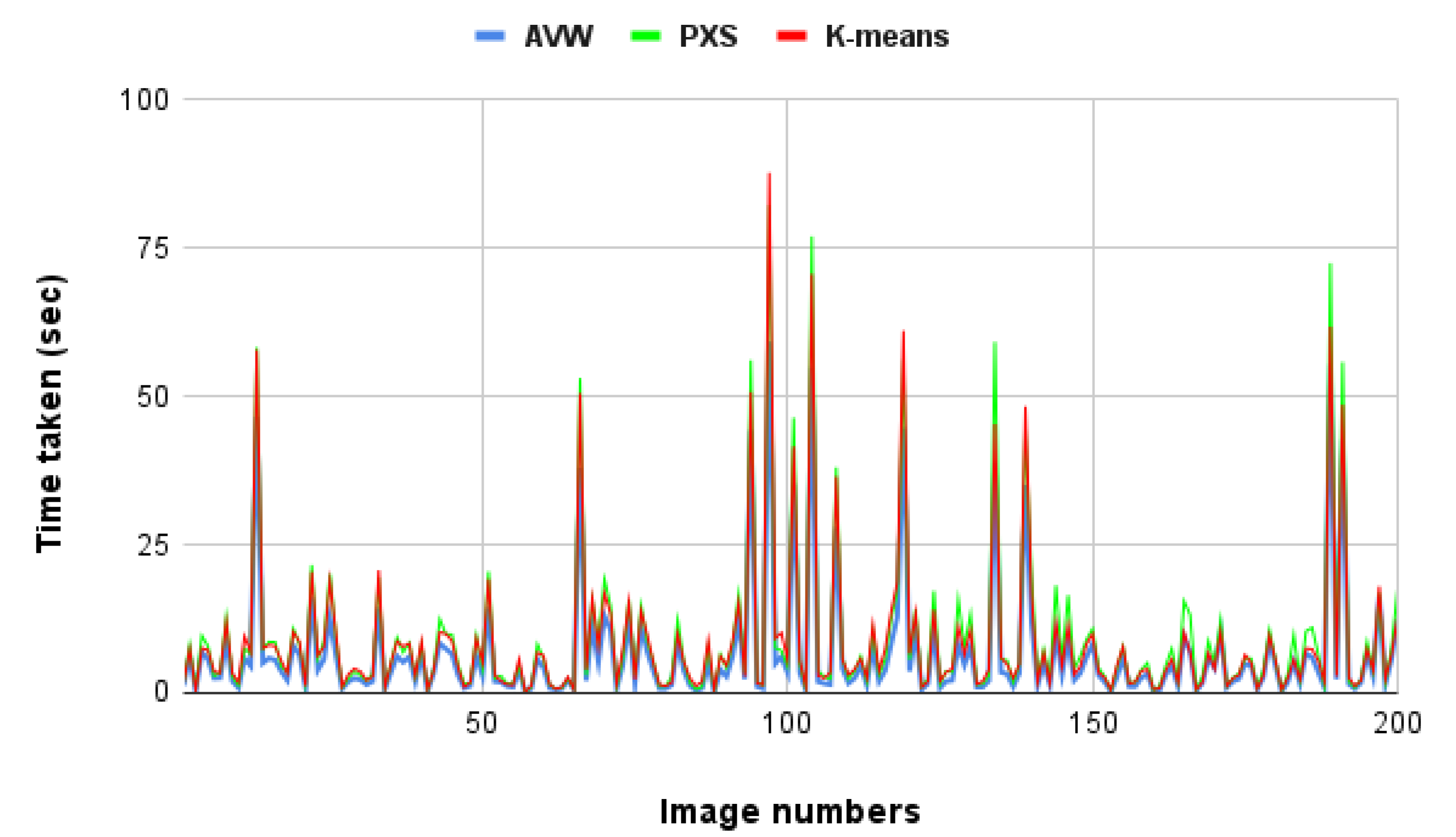
6.2. K-Means Clustering

In the domain of machine learning, K-means is one of the well-known unsupervised clustering algorithms. The algorithm, at random chooses “k” data points, called means. It then classifies the other data points into their nearest mean, by checking the Euclidean distance, and updates the mean value to the average of the cluster after each iteration of K-means. This process is repeated until the centroids of the clusters become equal for two simultaneous iterations. Many researchers have proposed modified versions of K-means approach, to improve the efficiency of K-means [39,40,41]. Hence, in order to evaluate the performance of the proffered algorithms, the K-means algorithm was tested for dominant color prediction with the benchmark data set. A plot of the time comparison between K-means and the AVW, PXS algorithms is displayed in Figure 10.

It can be inferred from Figure 10, that AVW handily outpaces K-means clustering in predicting the dominant color of objects. K-means draws less time than PXS. The accuracy of K-means for the benchmark data set is 84.1%, which is less compared to AVW and PXS. Hence, both the AVW and PXS algorithms outperform K-means clustering on accurate predictions of the dominant color of objects. The average time taken by the K-means for predicting the output for the benchmark data set is 8.7 s, versus 6.5 s for AVW. However, PXS takes a higher time, i.e., 0.5 s higher, compared to K-means as displayed in

Table 5. Comparison of normalized times for K-means, AVW and PXS schemes.

Algorithm	Minimum	Maximum	Mean	Standard Deviation
AVW	0.12	59.23	6.52	10.24
PXS	0.17	82.27	9.16	13.73
K-means	0.20	87.74	8.64	12.98

.

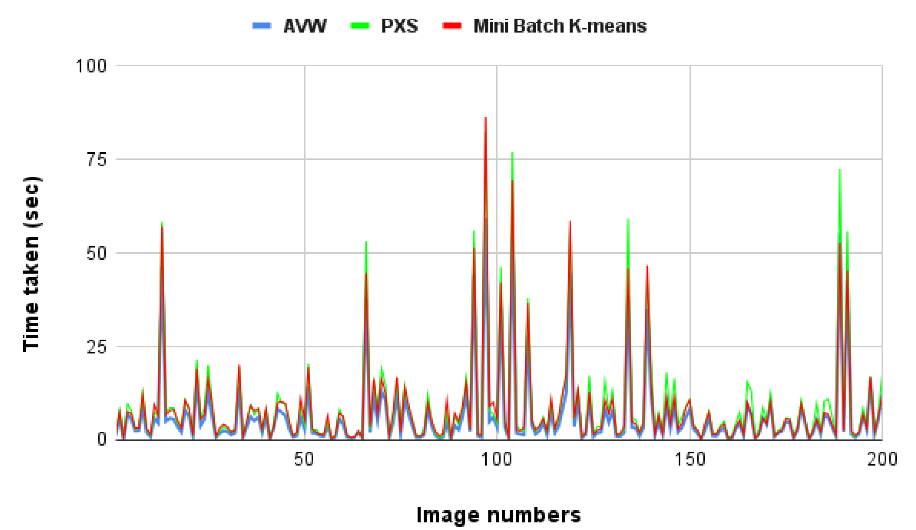
6.3. Mini Batch K-Means Algorithm

The time complexity of K-means increases for larger data sets [42]. Hence, alternative clustering algorithms, such as mini batch K-means, are introduced, which mitigate the spatial complexity of the algorithm. In mini batch K-means, small batches of data are processed as randomized. Mini batch K-means reduces the number of computations of distance per iteration, ensuing in additional decrease in the processing time of the algorithm. Mini batch K-means is implemented inside the masked regions of the input image that yield the maximum RGB value for each object. Color prediction is accomplished by the conversion of the RGB values into HSV equivalents. Figure 11 shows the time comparison plot for mini batch K-means and the proposed algorithms.

AVW performs color prediction in less time than mini batch K-means. The time taken for mini batch K-means is similar to that of K-means, whereas the accuracy of mini batch K-means is 83.8%, much less than the accuracy of both AVW and PXS algorithms. The average time taken by the mini batch K-means for predicting the output for the benchmark data set is 8.4 s compared to 6.5 s for AVW; however, PXS consumes a prediction time of 9.2 s as presented in

Table 6. Comparison of normalized times for mini batch K-means, AVW and PXS schemes.

Algorithm	Minimum	Maximum	Mean	Standard Deviation
AVW	0.12	59.23	6.52	10.24
PXS	0.17	82.27	9.16	13.73
Mini Batch K-means	0.24	86.43	8.39	12.55

. The effect of higher average time on the overall performance for PXS can be perceived as a trade-off for its higher accuracy.

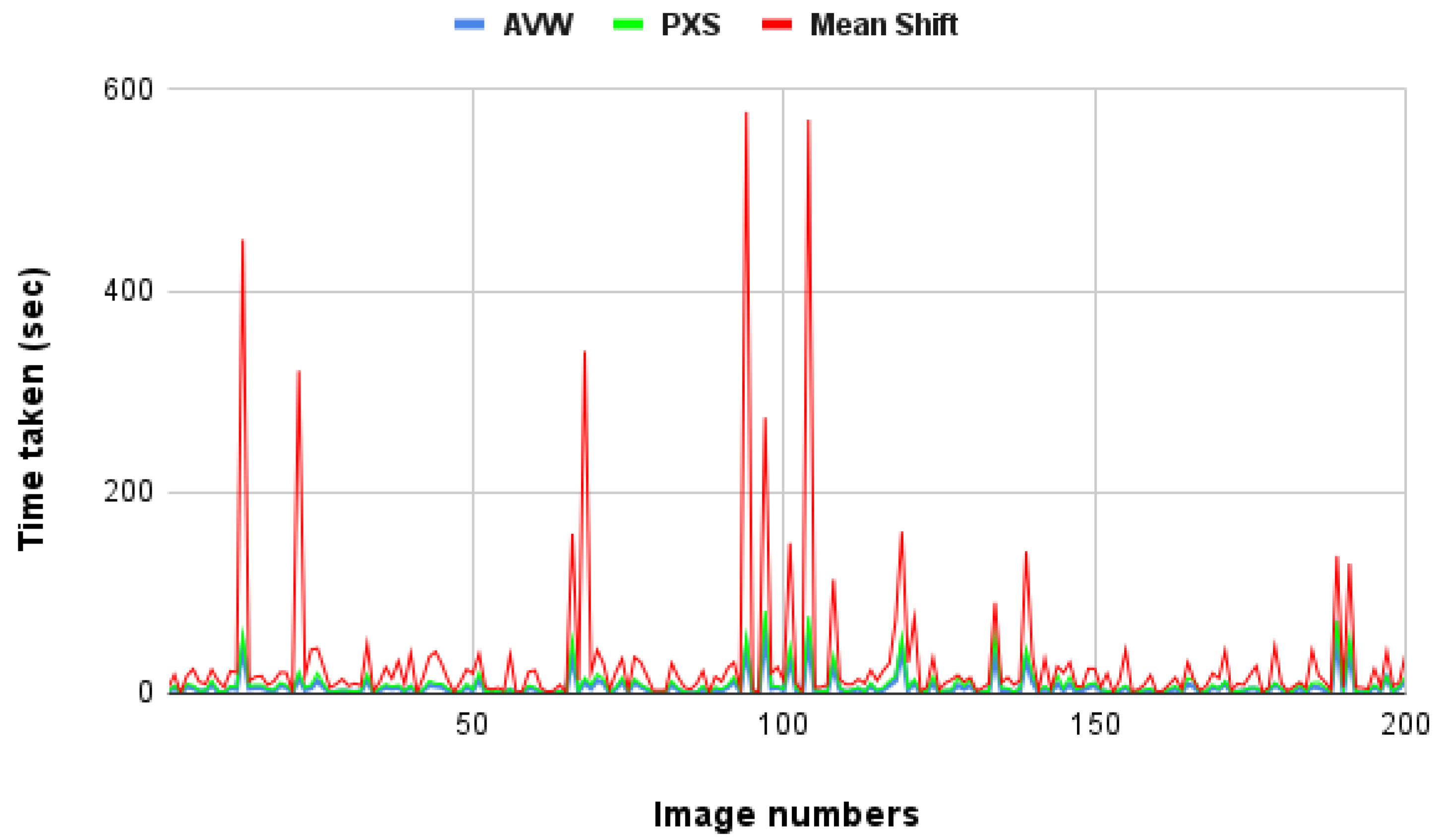
6.4. Mean-Shift Clustering

The mean-shift scheme continuously iterates data points by calculating their means, followed by relocation of the cluster’s center to the mean point. This process is repeated until there is a convergence, when the center of the cluster with the highest number of data points can be considered the dominant color. The algorithm was integrated with Mask R-CNN, and evaluated on the benchmark data set against the results with AVW and PXS. Time complexity, the major snag of the mean-shift algorithm, can be alleviated by considering selective data points for mean calculation [43]. The time comparisons for mean-shift and the AVW, PXS algorithms are shown in Figure 12.

The accuracy of mean shift for the benchmark data set is 85.2% which is less than that of AVW and PXS. Hence, both AVW and PXS outperform the mean shift algorithm in terms of time and accuracy for prediction of the dominant color of an image. The average time taken by the mean shift for predicting the output for the benchmark data set is 33 s—five times greater than that for AVW and easily three times higher than the time entailed by PXS as indicated in

Table 7. Comparison of normalized times for mean shift, AVW and PXS schemes.

Algorithm	Minimum	Maximum	Mean	Standard Deviation
AVW	0.12	59.23	6.52	10.24
PXS	0.17	82.27	9.16	13.73
Mean shift	0.30	577.93	32.93	76.66

.

6.5. Gaussian Mixture Model

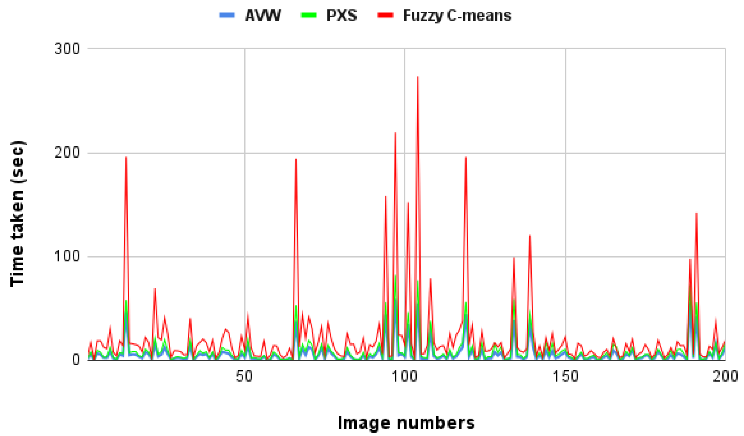
The Gaussian mixture model is a well-defined clustering algorithm that is used to classify a set of given data into clusters having common parameters. It uses Gaussian curves to assign the data points into different classes that yield a mixed representation of Gaussians. The Gaussian mixture model considers the probability by which a data point is assigned to one or more Gaussian curves. It is possible to have data points assigned under different clusters. It works similar to that of the K-means algorithm, but nets a better result in the quality and shape of the clusters. This algorithm is integrated with the DCPCM model for comparing accuracy and time complexity with AVW and PXS, which are summarized in Figure 13.

From the above plot, it can be deduced that the Gaussian mixture model imposes the highest burden on time compared to the AVW and PXS schemes. The Gaussian mixture model, when tested with the benchmark data set, delivered an accuracy of 88% in color prediction. The average time drained by the Gaussian mixture model for predicting the output for the benchmark data set is 13.4 s, as demonstrated in

Table 8. Comparison of normalized times for Gaussian mixture model, AVW and PXS schemes.

Algorithm	Minimum	Maximum	Mean	Standard Deviation
AVW	0.12	59.23	6.52	10.24
PXS	0.17	82.27	9.168	13.73
Gaussian mixture model	0.29	132.14	13.40	21.52

, notably higher than the time consumed by the AVW and PXS algorithms.

6.6. Fuzzy C-Means

Fuzzy C-means is an unsupervised clustering algorithm that analyzes various types of data and groups them according to their similarity [44]. It assigns membership value to each data point per cluster center, based on the Euclidean distance between the data point and center of the cluster. Rather than forcing a data point into one cluster, it assigns a data point to one or more clusters based on its membership value. Indicating partial membership and fuzzy partitioning, its value can range between 0 and 1 for different cluster centers. New cluster centers and membership values of each data point are computed for each iteration until convergence is encountered. The time comparisons for fuzzy C-means integrated with the DCPCM model and the proposed algorithms are shown in Figure 14.

According to the above plot, fuzzy C-means require more time for color prediction than AVW and PXS. The accuracy of color prediction with fuzzy C-means for the benchmark data set is 85.9%. AVW and PXS outperformed fuzzy C-means with respect to time and accuracy. The average times for prediction of the output by the fuzzy C-means with the benchmark data set is 22.4 s, compared to 6.5 s for AVW, and 9.2 s for PXS as shown in

Table 9. Comparison of normalized times for fuzzy C-means, AVW and PXS schemes.

Algorithm	Minimum	Maximum	Mean	Standard Deviation
AVW	0.12	59.23	6.52	10.24
PXS	0.17	82.27	9.16	13.73
Fuzzy C-means	1.36	273.48	22.41	38.85

.

Table 10. Comparison of time reduction and accuracies of all the discussed algorithms.

Algorithm	Color Prediction Accuracy (%)	Reduction in Time Compared to All-Pixel (%)
AVW	93.6	62
PXS	95.4	44.3
K-means	84.1	45.1
Mini batch K-means	83.8	47.5
Mean shift	85.2	−70.7
Fuzzy C-means	85.9	−53.4
Gaussian mixture model	88	22.4

represents the algorithm-specific prediction accuracy of an object’s color and time reduction compared to the all-pixel approach for the respective algorithm. Discernment of the results in Table 10 reveals the following:

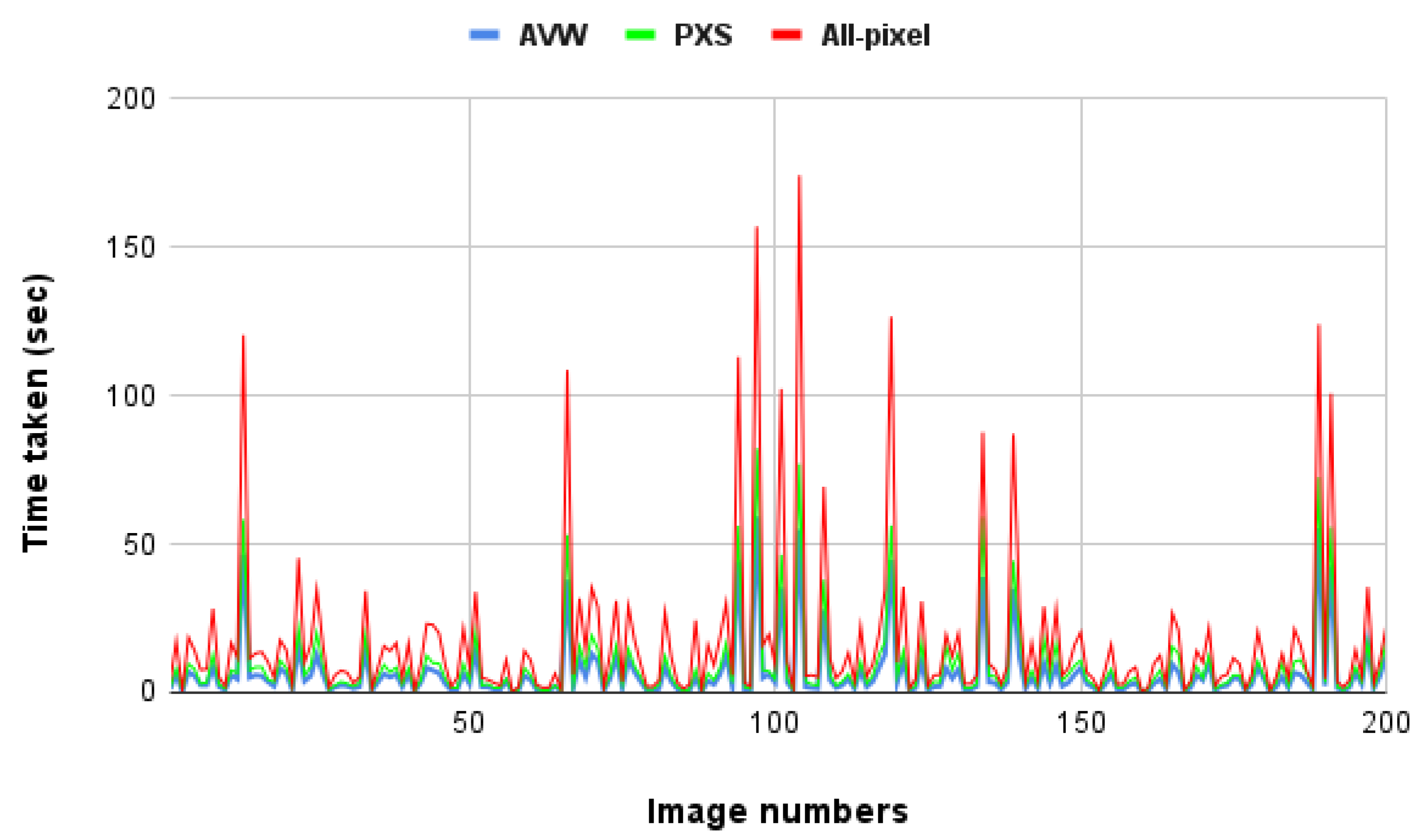
• AVW and PXS algorithms have higher accuracies compared to all other appraised algorithms;
• PXS algorithm is the most accurate among all the other clustering algorithms;
• AVW algorithm has the highest reduction in time along with decent prediction accuracy;
• Negative values of “reduction in time” for mean shift and fuzzy C-means algorithms imply that they require much longer than the all-pixel approach for the color prediction task.

7. Conclusions

Sustained proliferation in the deployment of autonomous robotic devices has stimulated enhanced urgency in their capability of detection and discernment of objects in an image. This paper has elucidated the design and working of two innovative color prediction algorithms, PXS and AVW, for the extraction of pixels in a faster and more efficient manner. Accuracy and reliability of the proposed algorithms are appraised by comparison of the proffered algorithms with conventional approaches—K-means, Gaussian mixture model, fuzzy C-means, mini batch K-means, and mean-shift clustering algorithms—using a benchmark data set. The propounded algorithms performed with greater accuracy in an exceptionally short time span, when AVW and PXS were juxtaposed with popular extant color prediction algorithms. AVW and PXS algorithms are distinct from each other. PXS algorithm exhibited enhanced accuracy (95.4%) with a downside of longer prediction time. The AVW algorithm perceptibly needed less time for prediction of an object’s dominant color (up to 62% decrease versus the all-pixel approach), incurring a compromised accuracy of up to 2%. A notable inference of this study calls for application-specific trade-offs between latency and prediction accuracy.

For color prediction, either AVW or PXS can be deployed; if time complexity is a major concern for predicting color, the AVW algorithm can be considered, which consumes an optimized time returning decent accuracy. If one prefers higher accuracy, PXS can be chosen for the color prediction, with a little higher prediction time compared to the existing techniques. Integration of the proposed algorithms with service robots can have a significant impact in detection of objects based on color in a real-time scenario. Time consumed to predict the color by these proposed algorithms is notably less than that of clustering algorithms. These algorithms are also useful for detecting traffic signals for autonomous vehicles and for detection of damaged foods. Clustering algorithms are ill suited for real time scenarios, due to their twin problems of less accuracy and longer prediction times. The proposed DCPCM model can be deficient dealing with equally shaded multicolored objects as well as certain real-time applications. These apparent deficiencies call for additional research and development of the DCPCM concept to sustain higher precision and streamlined performance of AVW and PXS algorithms.

References

1. Kim, J.H.; Kim, B.G.; Roy, P.P.; Jeong, D.M. Efficient Facial Expression Recognition Algorithm Based on Hierarchical Deep Neural Network Structure. IEEE Access 2019, 7, 41273–41285. [Google Scholar] [CrossRef]
2. Jeong, D.; Kim, B.-G.; Dong, S.-Y. Deep Joint Spatiotemporal Network (DJSTN) for Efficient Facial Expression Recognition. Sensors 2020, 20, 1936. [Google Scholar] [CrossRef] [PubMed]
3. Kim, J.-H.; Hong, G.-S.; Kim, B.-G.; Dogra, D.P. deepGesture: Deep learning-based gesture recognition scheme using motion sensors. Displays 2018, 55, 38–45. [Google Scholar] [CrossRef]
4. Manju, K.; Aditya, G.; Ruben, G.C.; Verdú, E. Gesture Recognition of RGB and RGB-D Static Images using Convolutional Neural Networks. Int. J. Interact. Multimed. Artif. Intell. 2019, 5, 22–27. [Google Scholar] [CrossRef]
5. Qummar, S.; Khan, F.G.; Shah, S.; Khan, A.; Shamshirband, S.; Rehman, Z.U.; Khan, I.A.; Jadoon, W. A Deep Learning Ensemble Approach for Diabetic Retinopathy Detection. IEEE Access 2019, 7, 150530–150539. [Google Scholar] [CrossRef]
6. Shamshirband, S.; Mahdis, F.; Dehzangi, A.; Chronopoulos, A.T.; Alinejad-Rokny, H. A review on deep learning approaches in healthcare systems: Taxonomies, challenges, and open issues. J. Biomed. Inform. 2021, 113, 103627. [Google Scholar] [CrossRef]
7. Pillai, M.S.; Chaudhary, G.; Khari, M.; Crespo, R.G. Real-time image enhancement for an automatic automobile accident detection through CCTV using deep learning. Soft Comput. 2021, 25, 11929–11940. [Google Scholar] [CrossRef]
8. Pathak, A.R.; Pandey, M.; Rautaray, S. Application of Deep Learning for Object Detection. Procedia Comput. Sci. 2018, 132, 1706–1717, ISSN-1877-0509. [Google Scholar] [CrossRef]
9. Liu, L.; Ouyang, W.; Wang, X.; Fieguth, P.; Chen, J.; Liu, X.; Pietikäinen, M. Deep Learning for Generic Object Detection: A Survey. Int. J. Comput. Vis. 2020, 128, 261–318. [Google Scholar] [CrossRef]
10. Srisuk, S.; Suwannapong, C.; Kitisriworapan, S.; Kaewsong, A.; Ongkittikul, S. Performance Evaluation of Real-Time Object Detection Algorithms. In Proceedings of the 2019 7th International Electrical Engineering Congress (IEECON), Hua Hin, Thailand, 6–8 March 2019; pp. 1–4. [Google Scholar] [CrossRef]
11. Kim, J.-A.; Sung, J.-Y.; Park, S.-H. Comparison of Faster-RCNN, YOLO, and SSD for Real-Time Vehicle Type Recognition. In Proceedings of the 2020 IEEE International Conference on Consumer Electronics—Asia (ICCE-Asia), Seoul, Republic of Korea, 1–3 November 2020; pp. 1–4. [Google Scholar] [CrossRef]
12. Liu, Z.-Y.; Ding, F.; Xu, Y.; Han, X. Background dominant colors extraction method based on color image quick fuzzy c-means clustering algorithm. Def. Technol. 2020, 17, 1782–1790. [Google Scholar] [CrossRef]
13. Elavarasi, S.A.; Jayanthi, J.; Basker, N. Trajectory Object Detection using Deep Learning Algorithms. Int. J. Recent Technol. Eng. 2019, 8, C6564098319. [Google Scholar] [CrossRef]
14. Canny, J. A Computational Approach to Edge Detection. IEEE Trans. Pattern Anal. Mach. Intell. 1986, 8, 679–698. [Google Scholar] [CrossRef]
15. Kaggle. Ideas for Image Features and Image Quality. Available online: https://www.kaggle.com/code/shivamb/ideas-for-image-features-and-image-quality (accessed on 1 January 2022).
16. Vadivel, A.; Sural, S.; Majumdar, A.K. Human color perception in the HSV space and its application in histogram generation for image retrieval. In Color Imaging X: Processing, Hardcopy, and Applications; SPIE: Bellingham, WA, USA, 2005; Volume 5667. [Google Scholar]
17. Ray, S.A. Color gamut transform pairs. ACM Sig-Graph Comput. Graph. 1978, 12, 12–19. [Google Scholar]
18. Atram, P.; Chawan, P. Finding Dominant Color in the Artistic Painting using Data Mining Technique. Int. Res. J. Eng. Technol. 2020, 6, 235–237. [Google Scholar]
19. Data Engineering and Communication Technology; Raju, K.S.; Senkerik, R.; Lanka, S.P.; Rajagopal, V. (Eds.) Advances in Intelligent Systems and Computing; Springer: Berlin/Heidelberg, Germany, 2020; Volume 1079. [Google Scholar] [CrossRef]
20. Guyeux, C.; Chrétien, S.; BouTayeh, G.; Demerjian, J.; Bahi, J. Introducing and Comparing Recent Clustering Methods for Massive Data Management on the Internet of Things. J. Sens. Actuator Netw. 2019, 8, 56. [Google Scholar] [CrossRef]
21. Sai Satyanarayana Reddy, S.; Kumar, A. Edge Detection and Enhancement of Color Images Based on Bilateral Filtering Method Using K-Means Clustering Algorithm. In ICT Systems and Sustainability; Advances in Intelligent Systems and, Computing; Tuba, M., Akashe, S., Joshi, A., Eds.; Springer: Singapore, 2020; Volume 1077. [Google Scholar] [CrossRef]
22. Peng, K.; Leung, V.C.M.; Huang, Q. Clustering Approach Based on Mini Batch K-means for Intrusion Detection System Over Big Data. IEEE Access 2018, 6, 11897–11906. [Google Scholar] [CrossRef]
23. Liu, N.; Zheng, X. Color recognition of clothes based on k-means and mean shift Automatic Detection and High-End Equipment. In Proceedings of the 2012 IEEE International Conference on Intelligent Control, Beijing, China, 27–29 July 2012; pp. 49–53. [Google Scholar] [CrossRef]
24. Mohit, N.A.; Sharma, M.; Kumari, C. A novel approach to text clustering using shift k-medoid. Int. J. Soc. Comput. Cyber-Phys. Syst. Int. J. Soc. Comput. Cyber-Phys. Syst 2019, 2, 106–118. [Google Scholar] [CrossRef]
25. Balasubramaniam, P.; Ananthi, V.P. Segmentation of nutrient deficiency in incomplete crop images using intuitionistic fuzzy C-means clustering algorithm. Nonlinear Dyn. 2016, 83, 849–866. [Google Scholar] [CrossRef]
26. Yin, S.; Zhang, Y.; Karim, S. Large Scale Remote Sensing Image Segmentation Based on Fuzzy Region Competition and Gaussian Mixture Model. IEEE Access 2018, 6, 26069–26080. [Google Scholar] [CrossRef]
27. Liu, Y.; Xie, Z.; Liu, H. An Adaptive and Robust Edge Detection Method Based on Edge Proportion Statistics. IEEE Trans. Image Process. 2020, 29, 5206–5215. [Google Scholar] [CrossRef]
28. Latha, N.S.A.; Megalingam, R.K. Exemplar-based Learning for Recognition & Annotation of Human Actions. In Proceedings of the 2020 9th International Conference System Modeling and Advancement in Research Trends (SMART), Moradabad, India, 4–5 December 2020; pp. 91–93. [Google Scholar] [CrossRef]
29. Wang, Y.; Luo, J.; Wang, Q.; Zhai, R.; Peng, H.; Wu, L.; Zong, Y. Automatic Color Detection of Grape Based on Vision Computing Method. In Recent Developments in Intelligent Systems and Interactive Applications IISA 2016; Advances in Intelligent Systems and, Computing; Xhafa, F., Patnaik, S., Yu, Z., Eds.; Springer: Cham, Switzerland, 2017; Volume 541. [Google Scholar] [CrossRef]
30. Zhou, S.; Wang, J.; Wang, L.; Zhang, J.; Wang, F.; Huang, D.; Zheng, N. Hierarchical and Interactive Refinement Network for Edge-Preserving Salient Object Detection. IEEE Trans. Image Process. 2021, 30, 1–14. [Google Scholar] [CrossRef] [PubMed]
31. Wang, L.; Tang, D.; Guo, Y.; Do, M.N. Common Visual Pattern Discovery via Nonlinear Mean Shift Clustering. IEEE Trans. Image Process. 2015, 24, 5442–5454. [Google Scholar] [CrossRef] [PubMed]
32. Liu, X.; Zhao, D.; Jia, W.; Ji, W.; Ruan, C.; Sun, Y. Cucumber Fruits Detection in Greenhouses Based on Instance Segmentation. IEEE Access 2019, 7, 139635–139642. [Google Scholar] [CrossRef]
33. Megalingam, R.K.; Sree, G.S.; Reddy, G.M.; Krishna, I.R.S.; Suriya, L.U. Food Spoilage Detection Using Convolutional Neural Networks and K Means Clustering. In Proceedings of the 2019 3rd International Conference on Recent Developments in Control, Automation & Power Engineering (RDCAPE), Noida, India, 10–11 October 2019; pp. 488–493. [Google Scholar] [CrossRef]
34. Megalingam, R.K.; Karath, M.; Prajitha, P.; Pocklassery, G. Computational Analysis between Software and Hardware Implementation of Sobel Edge Detection Algorithm. In Proceedings of the 2019 International Conference on Communication and Signal Processing (ICCSP), Chennai, India, 4–6 April 2019; pp. 529–533. [Google Scholar] [CrossRef]
35. Megalingam, R.K.; Manoharan, S.; Reddy, R.; Sriteja, G.; Kashyap, A. Color and Contour Based Identification of Stem of Coconut Bunch. IOP Conf. Ser. Mater. Sci. Eng. 2017, 225, 012205. [Google Scholar] [CrossRef]
36. Alexander, A.; Dharmana, M.M. Object detection algorithm for segregating similar colored objects and database formation. In Proceedings of the 2017 International Conference on Circuit, Power and Computing Technologies (ICCPCT), Kollam, India, 20–21 April 2017; pp. 1–5. [Google Scholar] [CrossRef]
37. Krishna Kumar, P.; Parameswaran, L. A hybrid method for object identification and event detection in video. In Proceedings of the 2013 4th National Conference on Computer Vision, Pattern Recognition, Image Processing and Graphics (NCVPRIPG), Jodhpur, India,, 20–21 April 2013; pp. 1–4. [Google Scholar] [CrossRef]
38. Molada-Tebar, A.; Marqués-Mateu, Á.; Lerma, J.L.; Westland, S. Dominant Color Extraction with K-Means for Camera Characterization in Cultural Heritage Documentation. Remote Sens. 2020, 12, 520. [Google Scholar] [CrossRef]
39. Khandare, A.; Alvi, A.S. Efficient Clustering Algorithm with Improved Clusters Quality. IOSR J. Comput. Eng. 2016, 48, 15–19. [Google Scholar] [CrossRef]
40. Wu, S.; Chen, H.; Zhao, Z.; Long, H.; Song, C. An Improved Remote Sensing Image Classification Based on K-Means Using HSV Color Feature. In Proceedings of the 2014 Tenth International Conference on Computational Intelligence and Security, Kunming, China, 15–16 November 2014; pp. 201–204. [Google Scholar] [CrossRef]
41. Haraty, R.A.; Dimishkieh, M.; Masud, M. An Enhanced k-Means Clustering Algorithm for Pattern Discovery in Healthcare Data. Int. J. Distrib. Sens. Netw. 2015, 11, 615740. [Google Scholar] [CrossRef]
42. Bejar, J. K-Means vs. Mini Batch K-Means: A Comparison; LSI-13-8-R. 2013. Available online: http://hdl.handle.net/2117/23414 (accessed on 1 January 2020).
43. Cheng, Y. Mean shift, mode seeking, and clustering. IEEE Trans. Pattern Anal. Mach. Intell. 1995, 17, 790–799. [Google Scholar] [CrossRef]
44. Hung, M.-C.; Yang, D.-L. An efficient Fuzzy C-Means clustering algorithm. In Proceedings of the 2001 IEEE International Conference on Data Mining, San Jose, CA, USA, 29 November–2 December 2001; pp. 225–232. [Google Scholar] [CrossRef]
Figure 1. System architecture of dominant color prediction using AVW and PXS algorithms. The output image in the given figure detected 5 objects along with the dominant color. The detection results in the output image (left to right) are as follows: gray dining table (0.974); cyan bowl (0.961); orange bowl (0.989); pink spoon (0.975); and red knife (0.989). The output format is as follows: dominant color of the predicted object, predicted object class (confidence score of the predicted object). Each detected object is surrounded by a bounding box.
Electronics 12 00909 g001
Figure 2. [Predicted and extracted] output images by the proposed AVW algorithm.
Electronics 12 00909 g002
Figure 3. [Predicted and extracted] output images by the proposed PXS algorithm.
Electronics 12 00909 g003
Figure 4. Different stages involved in color prediction, i.e., extraction of the pixels contributing to color prediction and the final output, using AVW and PXS algorithms.
Electronics 12 00909 g004
Figure 5. Color prediction results (final output with the color of the detected objects) using AVW algorithm.
Electronics 12 00909 g005
Figure 6. Color prediction results (final output with the color of the detected objects) using PXS algorithm.
Electronics 12 00909 g006
Figure 7. Standard deviation of time taken in each iteration of AVW.
Electronics 12 00909 g007
Figure 8. Standard deviation of time taken in each iteration of PXS.
Electronics 12 00909 g008
Figure 9. Comparison of color prediction time of all-pixel, AVW and PXS schemes.
Electronics 12 00909 g009
Figure 10. Time comparison plot of K-means, AVW and PXS.
Electronics 12 00909 g010
Figure 11. Time comparison plot of mini batch K-means, AVW and PXS.
Electronics 12 00909 g011
Figure 12. Time comparison plot of mean shift, AVW and PXS.
Electronics 12 00909 g012
Figure 13. Time comparison plot of Gaussian mixture model, AVW and PXS.
Electronics 12 00909 g013
Figure 14. Time comparison plot of fuzzy C-means, AVW and PXS.
Electronics 12 00909 g014