A Novel Ensemble Based Reduced Overfitting Model with Convolutional Neural Network for Traffic Sign Recognition System

Abstract

The ELVD (Ensemble-based Lenet VGGNet and DropoutNet) model is used in this paper to examine hypothetical principles and theoretical identification of a real-time image classification and object, tracking, and recognition device running on board a vehicle. Initially, we obtained the dataset from Kaggle. After loading the images, they were converted into 4D tensors and then into a grid. The model has to set the training to 70% training and 30% testing. The ELVD model uses 39,209 32 × 32-pixel color images for preparation, and 12,630 images specifically for research, in the GTSD (German Traffic Sign Detection) dataset. Each picture is a photograph of a traffic sign that corresponds to one of the 43 classes. The picture is a 32 × 32 × 3 sequence of pixel quality values in the RGB color region, defined as pixel values. The image’s class is hidden as a numerical value from 0 to 42. The image collection is somewhat unbalanced, and a few classes are represented significantly better than in the alternative model. The contrast and brightness of the images also differ significantly. The proposed model was created with CNN with Keras and applied with ensemble-based combined LeNet, VGGNet, and DropoutNet pooling layer for tuning the information. The proposed model compares the predicted class with the correct class for all input images and time calculation for predicting different road sign detection images. Underfitting is shown by a standard of low accuracy on the training and testing sets. For a small dataset, the trained model achieved a 98% accuracy level which implied that overfitting the model with the best results on classification accuracy, tested with 15 epochs, resulted in a loss of information of 0.059% and test accuracy of 98%, respectively. Next, the ELVD proposed models trained and validated with different class presents, dataset 2 achieved 93% training accuracy and testing accuracy predicted with 91%. Finally, the ELVD proposed model predicted the test results of unseen class information measured with the 60/km ph, which predicted 99% accuracy. The proposed model predicted noisy as well as unseen multiclass information with fast-moving vehicles. The usage of convolutional layer filter with ensemble-based VGGNet, DropouNet, and LeNet trained and predicted with a high classification accuracy of more than 99% combined ELVD model with fastest time calculation also the high accuracy prediction of selected image dataset labels that enables these models to be used in real-time applications. The ELVD model was also compared with other traditional models of VGGNet, LeNet, and DropoutNet; its detection time outperformed the other models, and it achieved a 98% detection label set of information. In the ELVD model, closure to various human abilities on a related responsibility differs from 97.3% to 99.5%; consequently, the ELVD model performs better than an average human.

1. Introduction

In recent years, machine learning has developed into a significant scientific field that has produced autonomous vehicles, speech recognition, and an increased understanding of the human genome. According to [1,2,3,4] interest is high partly because of the continuously rising volume and unpredictability of data and the cheaper and more potent computational processing. Utilizing algorithms to collect data, analyze it, and then generate predictions about the subject being studied is the fundamental idea of machine learning [2]. A huge amount of data is fed to the machine to teach it how to carry out the task rather than trying to manually code every operation. Deep learning, a subset of AI technologies, is a relatively recent research topic in machine learning.

In [2,3], they developed through deep learning, using a computational model called a neural network, which is inspired to some extent by the structure of the human brain. Neurons are the primary components of a neural network, which has various hidden layers. The neurons on the top layer are connected to the key, and the layers above it receive input. Self-driving vehicles and driver assistance are examples of real-world implementations for deep learning algorithms [4]. In the world of autonomous vehicles, the ability to correctly interpret traffic signals and take effective action is critical [5] In general, labeling and categorizing images has a wide range of applications for both academia and industry, making it a common and important research topic [6]. Deep learning emerged as a major subfield of machine learning science in 2006. It was labeled the hierarchical learning method by Mosavi and Varkonyi-Koczy, and provided pattern recognition fields of research. Deep learning of key factors, according to [7], is based on labeling or unlabeling Learning models for nonlinear implementation in separate phases with supervised learning, the category objective label is obtainable; moreover, the missing class target label handles an unsupervised method. During the ImageNet analysis of the high dimensionality recognition contest field in 2012 [8].

The German Traffic Sign Recognition Benchmark was used to train the VGG16 network using transfer learning and bottleneck features [9]. Synthetic aperture radar (SAR) delivers high-resolution, all-day, all-weather satellite imaging [10], which is ideally suited to better comprehend the marine domain and has grown to be one of the most significant methods for high-resolution ocean observation. We employ the free source SAR dataset LS-SSDD-v1.0 to develop and train a small vessel recognition model for computer vision that creates bounding boxes around ships. Automation of this kind would help regulatory bodies manage maritime traffic, fisheries, and shipwreck rescue operations more effectively. SAR images include a lot of noise, which makes it difficult to spot ships. Land clutter has an impact on ships docked at the port, making ship detection more challenging. Additionally, tiny ships are simple to overlook, whereas dense ships always appear as bright points in SAR photos, making it challenging to distinguish between different ships. The backscattered signal from ships is often substantially stronger than that from the sea surface [11]. In the SAR image, ships stand out more against the background. Therefore, it is possible to think about ship detection as looking for pixels in which the intensity level of the scattering signal is higher than the specified threshold.

Transfer learning is the process of repurposing a pre-trained network that was initially trained to recognize a wide range of image labels on a large amount of data to resolve a more complicated issue from a small number of features. The ELVD model resolves imbalances caused by training duplicate data and works optimal optimization to estimate the traffic sign. This technique uses deep neural networks to classify traffic indications more accurately. The proposed ELVD model predictions are shown in Figure 1.

The contributions of this work are summarized below.

• To use a complicated model to solve basic components and detect data noise.
• We initially began with a convolutional depth of 16 but found that 32 produced the best results. Gray scale often performed better than color when standard and normalized images were examined, as well.
• Large numbers of weight layers are possible with VGGNet using the small-size convolution filters, and more layers naturally result in better performance when predicting the exact traffic sign.
• Make the convolutional layers’ weights higher or equal to the probability of the fully connected layers. The way to approach this is to use the model to progressively compress it because it rejects too much information.

This section presents the Machine Learning classification as a whole. An innovative ensemble-based enhanced overfitting model is compared with a very imbalanced model in this article. The rest of this paper is organized as follows; Section 2 examines the background study CNN and Deep CNN with traffic sign detection, while Section 3 indicates problems identified unbalanced dataset. Section 4 describes the dataset using the ELVD model. Section 5 shows the system model ELVD approach. Section 6 indicates problem formation of the ELVD model. Section 7 describes the experimental results and analysis of training and testing for predicting traffic sign classification. Section 8 explains the future scope and enhancement of this extensive work.

2. Related Works

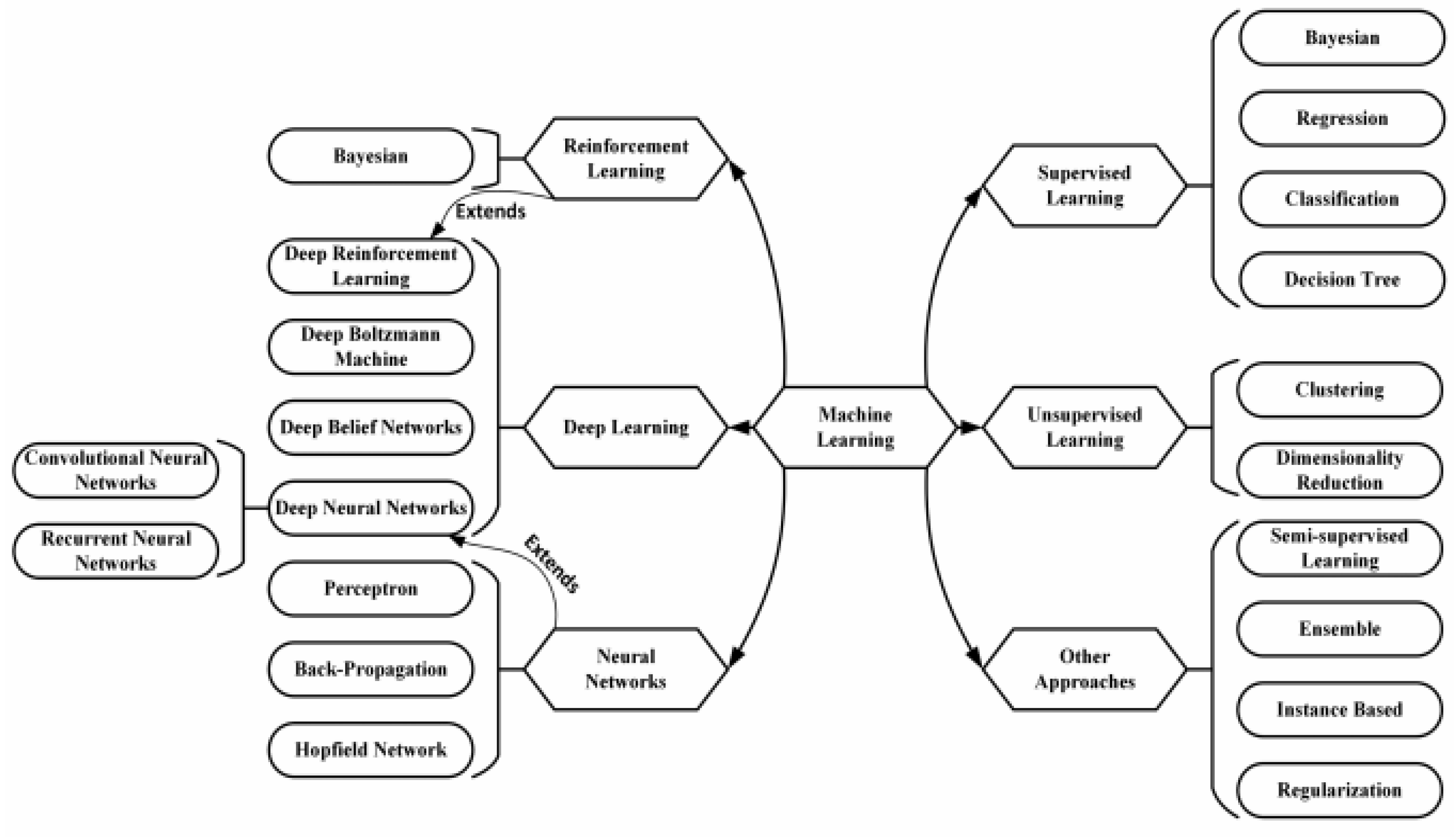
Deep learning is a form of machine learning that encompasses a wide range of techniques. Deep learning, unlike task-specific approaches, focuses on data perceptions by supervised, weakly supervised, and unsupervised learning. Deep learning approaches use a cascade of multiple layers of nonlinear processing units for feature extraction and manipulation. The data from the previous layer is used as feedback for each subsequent layer. Higher-level features are derived from lower-level features to form a hierarchical representation. Machine vision, speech recognition, and natural language processing all use deep learning models, which include deep neural networks, deep perception networks, and recurrent neural networks.

Perception and classification of traffic signals are essential in this phase and are needed for set automatic driving. The operation of traffic and road sign identification and designation has been the subject of extensive research. For traffic, the writers proposed using a CNN and SVM strategy. The authors applied 100,000 images to an advanced dataset and anticipated a traffic sign recognition and classification technique to be implanted on a stable end-to-end CNN. The system has an accuracy of 84%. The initial fuzzy classification approach was used to enhance classification and identification. Regulatory flags, alert signs, reference signs, and other signs are the four types of signs used in the United States. In the German GTSDB dataset, there are further signals from these three nations. Using a powerful end-to-end convolutional neural network, the authors [12] created a new dataset with 100,000 photos that includes a method for revealing traffic signs and multi-class classification (cnn). The system is 84% accurate. Traffic sign detection using a constrained multi-scale deconvolution network (MDN). The method’s accuracy was 99.1%. In [13], the authors took into account a convolution neural network investigation of different methods for classifying road traffic signs. In the lead-up to the test, the mechanism discovered the possible suggested approaches using CNN techniques in a specific time complexity and quality recognition.

In [14], they constructed an automated traffic and road sign recognition model, Deep Convolutional Neural Network (CNN) is used. This system cluster was developed to locate and classify traffic sign videos. The enhancement of this research is still a recently updated set of 24 different traffic signs gathered from the Saudi Arabian contingent road market. To manipulate the test images, various points and measuring with other factors and climatic contexts are used. A total of 2718 photographs were gathered from the dataset, with Saudi Arabian Traffic and Road Signs being one of them (SA-TRS-2018).

In [15,16], the authors explored the Extreme Learning Machine (ELM) mechanism, which uses innovative learning methods to break the hidden layer into ffn-feed forward neural networks. For greater statistics of unseen neurons, the ELM technique has been studied for improved execution with additional computing costs. The model uses traffic prediction to process executing this methodology for testing with HOG-related functionality [17]. Whereas the ELM model was used to establish the TSR system’s achievement, [18] chose an advanced trafficsign detection methodology based on classifying the color information allocated on steerable pyramid decomposition and the ELM model. To observe effective and detailed traffic sign identification and interpretation, researchers used [19] to simulate the model CNN for labeling the traffic sign system. The model progress, the advanced intention to implementation model, Edge Box, by cover consistently with a qualified Fully Connected Network as a result of the specificity of the traffic settings. The FCN-assisted object outline can achieve a more targeted capability, which can be used to prepare the aggregate detection model for fast and accurate detection. The proposed methodology was calculated on a widely used traffic sign parameter, the Swedish Traffic Signs Dataset (STSD), and the most recent result was obtained.

In [20], they discovered a number of alternative traffic sign acceptance approaches based on various classifiers such as the closest adjacent algorithm, Random Forests algorithm, neural networks, and SVM sustaining the [21]. Two neural networks continue to be educated and interpret the observed windows, according to [22,23] examined just at the root of HSI color first, then classified the objects using continuous SVMs balanced to type. To enable accurate identification procedures, each class is allocated a variety of SVMs. According to [24], an important 105 multilayer relationship dependent on CNN is easy to predict for traffic sign identification.

In the field of artificial intelligence, predicting accuracy is known as the additional amount of computation time required to process an image. When compared to other existing models, the proposed model has a faster computation time and a higher degree of accuracy. The latest developments are thoroughly examined in this paper’s literature analysis. As a result, it wishes to recommend an improved alternative to current methods of operation. One of the best strategies for solving real-world issues among the multi-class methodologies now in use is “one over one.” The suggested ELVD traffic sign identification method works effectively independent of whether the data contains overfitting information, and it predicts the accuracy label of 97 percent. These major limitations are addressed further in the study.

• The absence of techniques that address dim lighting.
• The lack of algorithms to deal with heavy snowfall and rain.
• No algorithms exist to deal with road signs under trees where various areas of the sign are exposed to varying degrees of light.

3. Problem with Over Fitting

In [25], the authors investigated the factors of overfitting or underfitting the data as the cause of improved efficiency in machine learning. Overfitting happens when a model learns the column and tests the improvement using errors from training samples, which has an uneven effect on the model’s performance on the original data. This method involves choosing and training the model’s interpretation of the noise or dependent variance in the training data samples. The concern is that these approaches do not relate to new data and diversely conflict with the model’s ability to generalize. Overfitting is a consistent error, as shown by the findings of the machine learning model on training data samples, which is distinct from the assessment, i.e., how adequately the model is applied to undetected data. There are two essential methods that the model can handle when assessing machine learning algorithms to define overfitting:

• To apply a resampling method to classify model accuracy.
• To carry back validation data samples.

According to [26], the crucial and appropriate resampling technique is k-fold cross-validation. It permits the model to train and test the k-times model on different subsets of training data samples, and it adds up an evaluation of the impact of a machine learning model on data samples that were not intended to be discovered. In [27] showed that validation samples are a detectable subgroup of the model training samples that we receive back from the model machine learning algorithms, which become the appropriate end of the prediction model. Following the selection and fine-tuning of machine learning algorithms on the training dataset, the learned models can be applied to the validation samples to obtain a final target understanding of how the models would perform on samples of undetected data. In [28], they ensembles are machine learning models for combining predictions from numerous conflicting models. There are several distinct methods for ensemble learning, though the two essential methods are [29]. Bagging attempts to scale down the likelihood of overfitting quality models. As such, it trains a considerable number of “adequate” learners. An active learner is a model that is about to be unreserved. Bagging associates the strong learners as beneficial in order to loosen their predictions. In [30], they stated that Boosting endeavors to better the predictive ability of complete models. It trains an enormous number of “weak” learners in continuance. [31] implied that Bagging handles complex base models and competes to “adequate” their future predictions, while Boosting consumes entire base models and tests to “boost” their accumulated problem.

4. Experimental Setup

The German traffic sign recognition benchmark (GTSRB), according to [32,33] and Kaggle, consists of color images of traffic signs (one sign per image), with image sizes ranging from 15 × 15 to 250 × 250 pixels. The training dataset consists of 39,209 color images, while the evaluation dataset consists of a total of 12,630 images. A variety of distant data-improving strategies is advantageous to match the number of training samples in separate classes further to advance the observation of the evolving network, including rotation, flipping, sharpening, Gaussian blur, motion blur, HSV intensification, and mirroring. An illustration of one of the 43 different kinds of traffic signs. Both images are confined and resized to 4848 pixels, as this is the best way to characterize the performance using GTSRB. On the GTSRB test dataset, the top-1 accuracy was calculated to determine the network’s accuracy.

5. System Model

This research predicts the accuracy of a huge dataset using GTSRB and TSRD data samples by applying various models to yield the distant EPOC time generated. We employ the ensemble technique to combine the three models accurately in ELVD resembles.

5.1. Regularization

In research article [33,34] suggested that, regularization is any improvement that a model makes to a learning system that is determined to fully truncate its prediction error rather than its prediction performance. A well-known regularization is repeatedly effected by assigning new constraints over a machine learning approach, essentially computing the constraints on the parameter values or enumerating extra terms in the intention function that can be considered equivalent to a convenient limitation on the parameter numerical values. Thus, precisely selected parameters can ensure minimal model testing inaccuracy results. L1 and L2 are the maximum moderate types of regularization. This revised information is the general cost function that accumulates distinct terms defined as the regularization terms.

Once the regularization term has been obtained, the numerical values of weight matrices reduce because it accepts that a neural network with lesser weight matrices has been applied to the basic models. Consequently, it will also reduce overfitting. Moreover, this regularization term contrasts in L1 and L2.

$$\mathrm{Loss} = Error (y,\overline{y})+\lambda {\displaystyle \sum }_{i=1}^N\left|{\omega }_{\mathrm{i}}\right|$$

(1)

$$L1=Cost \mathrm{Function} = \mathrm{Loss} +\frac{\lambda }{2m} * {\displaystyle \sum ‖\mathrm{w}‖}$$

(2)

Lambda is the regularization parameter value. It is the hyper parameter value that allows for improved results. L2 regularization is also acknowledged as weight consume as it causes the weights to dissolve close to zero.

$$L2=Cost \mathrm{Function} = \mathrm{Loss} +\frac{\lambda }{2m} * {{\displaystyle \sum ‖\mathrm{w}‖}}^2$$

(3)

In [35,36,37], they showed that, Dropout is extraordinary, which will have a major impact on the classification model. As aggregated weights in CNN layers are acceptable regularizes, the model normally drops out to completely connected layers. Although, a minimum improvement in attainment occurs when using a chunk of dropout on convolutional layers. L2 Regularization uses a lambda value of 0.0001 which implies improved execution has been achieved. The necessary details are superior to L2 loss, which will add weights of the fully connected layers, and consistently it does not contain bias boundary. Early stopping is a cross-validation scheme that uses one element of the training set to take one element of the validation set into the validation process. Considering the probability that the validation set’s attainment is insufficient, we immediately avoided training the model. Early stopping with a persistence of 100 epochs to detain the last outstanding weight effects and reduce as the model leaves over suitable training data set samples is recommended. As an early stopping metric, the model value validates the collection of cross entropy loss. Overfitting can be a serious issue in Deep Learning prediction models, as they have so much adaptability and size if the training dataset samples are small.

5.2. LeNet-5

According to [35,36,37,38], convolutional neural networks were created to precisely observe visual models from pixel images with minimal preparation. They are able to spot highly variable patterns. LeNet-5, is a recent convolutional network used for character recognition in printed text and handwriting. LeNet-5 uses seven-layer CNN architecture. Three convolutional layers, two subsampling layers, and two fully linked layers make up the layer content.

Figure 2 illustrates in more detail the architecture of LeNet-5 [35] the Convolutional Neural Network used in the simulation has seven layers, not including the data, all of which can be trained with numerical values (weights); a 32 × 32-pixel image is used as the input. This character is of a higher quality than the maximum in the character repository.

Algorithm

Step 1: Reading the data sample as LeNet-5 is a 32 × 32 (as shown in Figure 3) grayscale image that concedes due to the beginning CNN layer with six element maps or filters obtaining size 55% and an empty value of one. The image dimensions range from 32 × 32 × 1 to 28 × 28 × 6 pixels.

Step 2: The Second Layer—LeNet-5, adds a filter size of 2 × 2 and a stride of two to the mean numerical value of the pooling layer or sub-sampling layer. The picture will be compressed to 14 × 14 × 6 of its original size.

Step 3: Third Layer: This layer has a scale of 5 × 5, a stride of 1, and 16 convolutional components. Ten of the sixteen constituent maps in this layer are connected to the six attribute maps in the layer below.

Step 4: Typically, the Fourth Layer (S4) is a pooling layer with an average filter size of 2 × 2 and a stride of 2. With 16 function maps instead of the second layer’s (S2) two, this layer yields a value of 5 × 516.

Step 5: The Fifth Layer is a completely interconnected CNN layer that has 120 excellent maps that are exactly 1-1 in size. In particular, all 400 nodes (5 × 5 × 16) in the fourth layer of S4 are bound to the 120 units in C5.

Step 6: Sixth Layer—with 84 units, the sixth layer is a totally connected layer (F6).

Step 7: Last but not least, there is a softmax output layer that is fully connected and has ten conceptual values for the digits that can be assigned a range from 0 to 9.

5.3. VGGNet

ImageNet [36] is a general framework for labeling and classifying images into about 22,000 different object groups for computer vision processing. ImageNet collaborated with CNN for the Large Scale Visual Recognition Challenge or ILSVRC. According to [37], the goal of this image classification job is to train a model that can reliably classify and load the image into 1000 distributed item groups. 1.2 million training images, 50,000 evaluation images, and 100,000 model testing images are used to train the models. The advanced pre-trained systems, together with the Keras value library, have accomplished some of the unparalleled performing CNN on the ImageNet demands over the previous several years. The framework also demonstrated a secure ability to generate images outside the ImageNet dataset using transfer learning techniques, including extracting features & fine tuning hyper parameter values [38], seems how the VGG network architecture could be used to create a deep CNN for image recognition. Three convolutional layers that were created by stacking calculations together show the model’s clarity region. Decreasing content size is organized by the max pooling layer. A softmax classifier is followed by two fully connected layers that each has 4096 nodes, according to [39,40] that the VGG16 and VGG19 training datasets are proactive. VGGNet has two major drawbacks: it is incredibly difficult to practice, and the network architecture measurements themselves are a massive dataset.VGG is concluded with 533 MB for VGG16 and 574 MB for VGG19 as a result of its intensity and number of fully-connected nodes. As a result, setting up VGG is a time-consuming process. VGG, on the other hand, is often more appropriate in many deep learning image recognition problems for narrower network architectures. The original VGGNet (as shown in Figure 4) architecture contains 16–19 layers; The model carries out an altered version of the exclusive 12 layers to save computational edge. For more details on LeNet-5 and VGCNet we refer to [41,42,43,44,45,46].

Algorithm

Step 1: Initially, VGG proceeds in a 224 × 224 pixel RGB image. In the ImageNet contentions, the authors confined out the midpoint of 224 × 224 reconstructions in particular images to preserve the compatibility of input image size.

Step 2: The convolutional layers in VGG need an appropriate, limited perspective field (3 × 3, the essential accessible size that fixes occupy left or right and up or down). Additionally, 1 × 1 convolution filters measure a linear variation of the input data, which is ensured by a ReLU unit. The convolution limit is defined as 1 pixel such that the structural resolution is defined as eventually convolutional.

Step 3: The Fully Connected Layers. VGG acquires three fully connected layers: the first two carry 4096 handlings each, and the third holds 1000 consecutions, one for eachspecific class.

Step 4: In hidden Layers of VGGs, concealed layers select ReLU (an enormous correction from AlexNet-specific cut attainment time). VGG is not sufficient for the main use of Local Response Normalization in the model process, adding memory utilization and training time in addition to the choice of accurate build-up.

5.4. DropoutNet

A completely connected layer retains closest to the parameters, and as a result, neurons develop each range of training that limits the specific ability of each neuron due to over-fitting of the training phase [40]. The technique, called dropout, was created from the ground up to address the issue of inadequate training data harvests and overfitting. Dropout mechanisms briefly discard different units (both hidden and detectable) in the neural network, especially those reserved on the network. The dropped participants are excluded from the forward and backward propagation. When an observation is made, this generates a neural network sample with several architectures. According to [41], the dropout aspects of the system’s co-variations in the neural network are important since a unit cannot fully calculate the aspect of another specific to unit because that unit may be dropped out. The network becomes more effective through this process. A deep neural network applied to dropout produces a weak network comprised of all the units impacted by the dropout.

5.4.1. Forward Propagation with Dropout

Dropout is a generally used regularization mechanism in order that is explicit to deep learning. It randomly chooses to reserve certain neurons in respective iterations.

• To construct a variable d1, including the associated shape acting as 1, numbers are randomly obtained between 0 and 1 (1—carry probability) by thresholding values in D|1| with respect to the random matrix.

  $$D^1=\left[a{1}^{\left|1\right|(1)}a{1}^{\left|1\right|(2)}....a{1}^{\left|1\right|(m)}\right]$$

  (4)
• To conclude, each access of $D^1$ is to be 0 in connection with feasibility (1-keep_prob) or 1 as well as the probability (keep_prob) of reaching threshold numerical values in $D^1$, respectively. To conclude, all the access of a matrix X to 0 (if the approach is less than 0.5) or 1 (if the entry is higher than 0.5), choose: X = (X < 0.5). Indicate that 0 and 1 are consequently identical to False and True.
• To set A[1] to A[1]∗,$D^1$, is concluded with some of the numerical values.
• Divide A[1] by keep_prob. This step ensures that the cost will match the identical normal value considering the drop-out.

5.4.2. Backward Propagation with Dropout

In ackward propagation with dropout to develop the hidden layer vector, weight’s matrix, output layer vector, and the hidden weight’s matrix [42]. The model selects the number of secret autoencoders for the hidden layer. The output layer must obtain a set of activation functions proportional to the number of tests.

• To ensure prescient interruption with part of the neurons throughout forward propagation, it implements a mask ${\mathrm{D}}^1$ to A1. The modern back-propagation needs to choose the same neurons by reemploying the identical mask ${\mathrm{D}}^1$ to dA1.
• Throughout forward propagation, we include and split A1 by keep_prob. By back-propagation, the model needs to divide d$A^1$ by keep_prob repeatedly (the mathematic analysis of this is well-known; if A[1]A[1] is measured by keep_prob, then it is acquired d$A^1$.

Back-propagation neural networks execute well on huge datasets. The efficiency can be enhanced by developing the total number of hidden neurons along with the training rate. As a result of its continual training and gradient stored training, the acceptance rate is considerably behind the needs, so it reserves a huge measure of time to train on a huge dataset.

5.5. ELVD Proposed Diagram

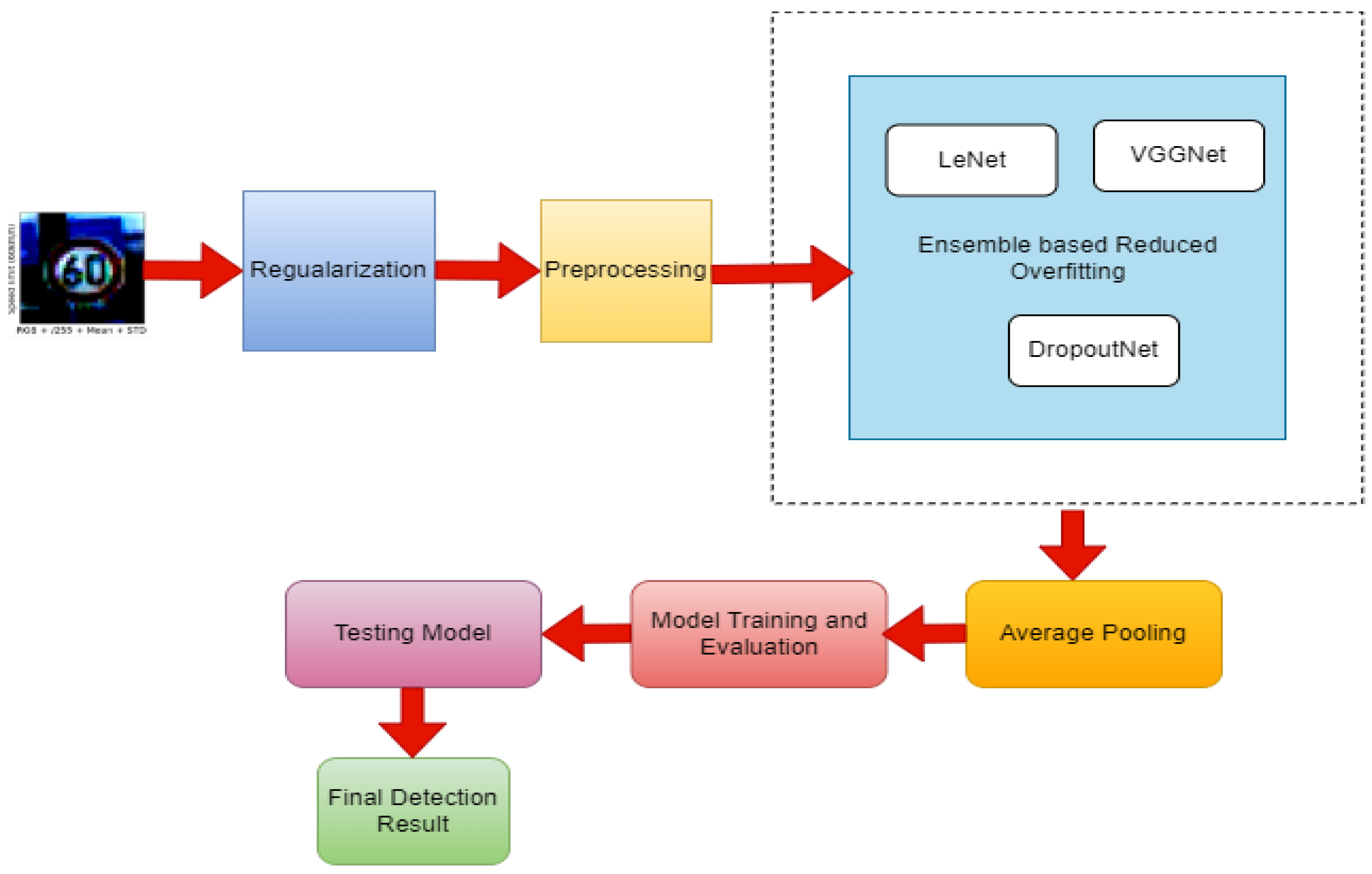
One of the best strategies for solving real-world issues among the multi-class methodologies is “one over one.” The suggested ELVD traffic sign identification method works effectively independent of whether the data contains overfitting information, and it predicts the accuracy label of 97 percent. Figure 5, shows the proposed ELVD Diagram.

5.6. Ensemble Based LeNet VGGNet and DropoutNet (ELVD) with CNN

• A 3-D volume calculation is developed for a specific substrate. The dimension that resolves is H*W*C. Height, width, and the overall number of channels are handled differently by H, W, and C.
• The K filter can be shortened, with K serving as the extended sum of the output value. The quality of all K filters is given by f*f*C, where f is the filter size, and C is the sum of the quality of the medium input image.
• Set up the padding according to the input padding volume. One row and one column will be calculated on either side of the aspect if padding is set to the same amount, and the aspect’s numerical value will be 0. Padding is acceptable anywhere along an input element’s height and width and is associated across all layers.
• The measurement produces a slide filter improvement from the top left edge after padding. All the replicated values are then taken into account after aggregating the equivalent filter and input volume values. The filter is now sliding horizontally based on the amount of stride moves in a given step. This way, if the stride is two, two columns can be slid horizontally. Until the image volume is hidden, the similar phase is occupied vertically.
• The RELU is activated to produce the subsequent values of the filter data processing after the collection of all previous values, which is the maximum (0,x). To ensure that the pixel has no association, zero retrieves all negative numerical values inside as negative data values.
• The 3-D input volume is changed to a 2-D volume as the output value via steps 4 and 5, which only produce one layer as the output value.
• For K filters, steps 4 and 5 have the same outcome. Additionally, the output of a unique filter is merged with the one mentioned before, changing the depth of the output picture computation of k.

To direct all the hyperparameters of a convolutional layer, compute the aspect of an output number. Any filter is reduced at this layer, conditioned, and initialized with erroneous minimal numbers. An output volume’s height and weight are determined by:

Height & weight = floor((W + 2∗P − F)/S +1)

(5)

depth = K (number of filters used)

(6)

6. Problem Formation Proposed Solution

6.1. Problem Formation

As a result of the object recognition and understanding credentials of humans, it is difficult to begin a computer-based classification that considers providing for people in regular activity. A group of conditions alter repeated functioning, such as brightness and perceptibility, which are resolved by the human recognition scheme together with simplicity; however, it results in essential disputes for computer-based identification. Furthermore, still images obtained from an ambient camera may contain blurred moving objects. Moreover, these images can consist of road traffic signs that are incompletely or entirely obscured by alternate objects such as vehicles or pedestrians. Further research has identified issues with the closeness of objects related to road signs; similarly, buildings or signboards can alter the model; therefore, creating a sign detection model is challenging. The system must deal with traffic and road signs in a broad range of weather conditions, with different environments serving as distinct remodels; various weather situations, such as sun, fog, rain, and snow must be considered.

6.2. Proposed Solutions

Often, word recognition is reduced to select a well-known sign classified during word classification to show that the sign is assigned to a secure category based on valid features. Previous classification issues have been considered as binary classification obstacles. Methods have been suggested to resolve multi-class research issues. The most convenient methods for practical disputes generate i(i-1)/2 classifiers, where I is the classification number. To solve the binary classification problem, samples are separated into two separate classes, the m^th and n^th classes, in particular, classifier trains.

$$Minimiz{e}_{\epsilon ,w,b }=\frac{1}{2}{w}^{m,n}.w^{mn}+C{\displaystyle \sum }_{i=1}^{}\epsilon i^{mn}$$

(7)

Ensemble learning is a machine learning approach where several learners are trained to clarify an identical problem, and their predictions are mixed with a single amount that reasonably has more complete attainment on the medium than any specific ensemble segment. The basic idea of successful ensemble learning is to combine delegated learners into one; a secure learner is less susceptible to error and is less vulnerable to overfitting in the presence of noise or limited model size.

7. Result and Discussion

Traffic Sign Classification, which uses CNN to separate the various class codes, is widely used in Artificial Intelligence, Machine Learning, and Deep Learning systems. Traffic recognition is a method of classifying traffic signs that automatically detect the lane and the speed limit, as well as yield, merge, and other signs. The accuracy of automatic recognition is predicted by the traffic signs when they are present.

Traffic sign recognition is the major research issue in computer vision, and deep learning can rectify the research issues based on an ensemble-based learning approach using CNN. The standard dataset used to train traffic sign classifiers is the GTSRB dataset, and the signs are separate from the traffic sign Region of Interest. The sign is classified in a two-stage process:

• Localization: Detection and localization of the traffic sign image.
• Recognition: To identify the traffic sign picture and calculate the ROI.
• The GTSRB dataset has a variety of issues, including low resolution and poor contrast. In order to train the traffic sign classifier effectively.
• Increase the contrast of our input images by preprocessing them.
• Take into account the skew of class labels.

In EDA, the selected files are used to receive the object of the German Traffic Signs Dataset. Matplotlib is a great resource for performing visualizations, and it was used to plot the traffic sign images and count each sign.

Figure 6 shows imbalanced images with highly imbalanced distributions consisting of 43 labels.

7.1. Model for Training and Testing Evaluation

The proposed ELVD model detects the traffic sign using RGB to understand the machine, the pixel information is then converted into numbers. For manipulating many image tasks, the ML uses the PIL library. The RGB images consist of different heights and widths. For this purpose, the ELVD manipulating task needs to resize the image to a fixed size of 30 × 30. The ELVD model is used to observe the shape of the entire information consisting of 3,920,930,303 and 39,209. For training the ELVD model to generate random input of different classes, the multiclass label ranges from 0 to 42 by applying CNN to encode the different sets of images with one-hot encoding to produce the element of the vector 0 and 1. [45] After the preprocessing steps, the model splits the shape into training and testing. The training shapes are as follows x_train = 3,136,730,303 and y_train = 31,367. The testing shape consists of x_test = 784,230,303 and y_test = 7842.

The model chose one traffic sign preprocessed in four different ways, with Figure 7a–d describing 3-channel preprocessed images in four different ways. The preprocessing steps included overfitting the data in the RGB dataset and ELVD model training the data samples with 100 and validated with 4410 samples. After the successful performance of the 15 Epochs, accuracy and loss rates were generated for predicted image samples.

On the GTSRB dataset, we checked the three CNN constructs to demonstrate the performance of our classification process. The GTSRB dataset was divided into testing and test datasets for analysis and assessment. For 15 traffic sign groups, we used 8970 images for preparation and 2790 for research in the CNN for triangular traffic sign identification. For 20 traffic sign groups, we used 22,949 images for preparation and 7440 images for research in the CNN for circular traffic sign identification. Finally, we used 39,209 images for preparation and 12,630 images for checking the CNN for total traffic awareness.

Table 1. ELVD model with a CNN trained dataset in 15 epochs.

Dataset	Epoch	Loss Rate	Accuracy Rate	Val_loss	Val_acc	Elapsed Time
GTSRB	1	2.531	0.380	0.951	0.782	78 s
	2	0.969	0.724	0.354	0.918	80 s
	3	0.591	0.831	0.174	0.960	78 s
	4	0.435	0.875	0.136	0.969	78 s
	5	0.370	0.894	0.122	0.969	78 s
	6	0.302	0.911	0.121	0.969	80 s
	7	0.277	0.920	0.090	0.902	78 s
	8	0.259	0.927	0.068	0.948	78 s
	9	0.237	0.933	0.108	0.973	78 s
	10	0.266	0.925	0.068	0.973	80 s
	11	0.240	0.933	0.068	0.982	78 s
	12	0.204	0.942	0.055	0.985	77 s
	13	0.204	0.944	0.054	0.984	78 s
	14	0.204	0.944	0.054	0.984	78 s
	15	0.177	0.950	0.059	0.985	79 s

shows the effects of using various layers to identify traffic signs in CNN, along with the error rate, accuracy rate, validation error, and validation accuracy measured using 15 EPOC. The number of iterations the machine learning algorithm has completed across the full training dataset is referred to as an epoch in this context.

Batches are generated from a vast number of datasets. The dataset correlation size is d, the number of epochs is e, the number of repetitions is I, and the batch size is b, therefore, the epoch equation can be written as d*e = i*b.

• For both training sets, 1 Epoch equals 1 Forward pass + 1 Backward pass.
• Batch size refers to the number of training samples used in a single Forward/1 Backward pass.
• The number of loops equals the number of moves, measured as 1 Pass = 1 Forward + 1 Backward pass.
• The unseen training samples of 15 EPOC trained the accuracy level presented in 98%.

Figure 8 shows the overfitting of small data for the RGB dataset-2 trained and validated the samples shows the accuracy level indicated with increasing the trained information.

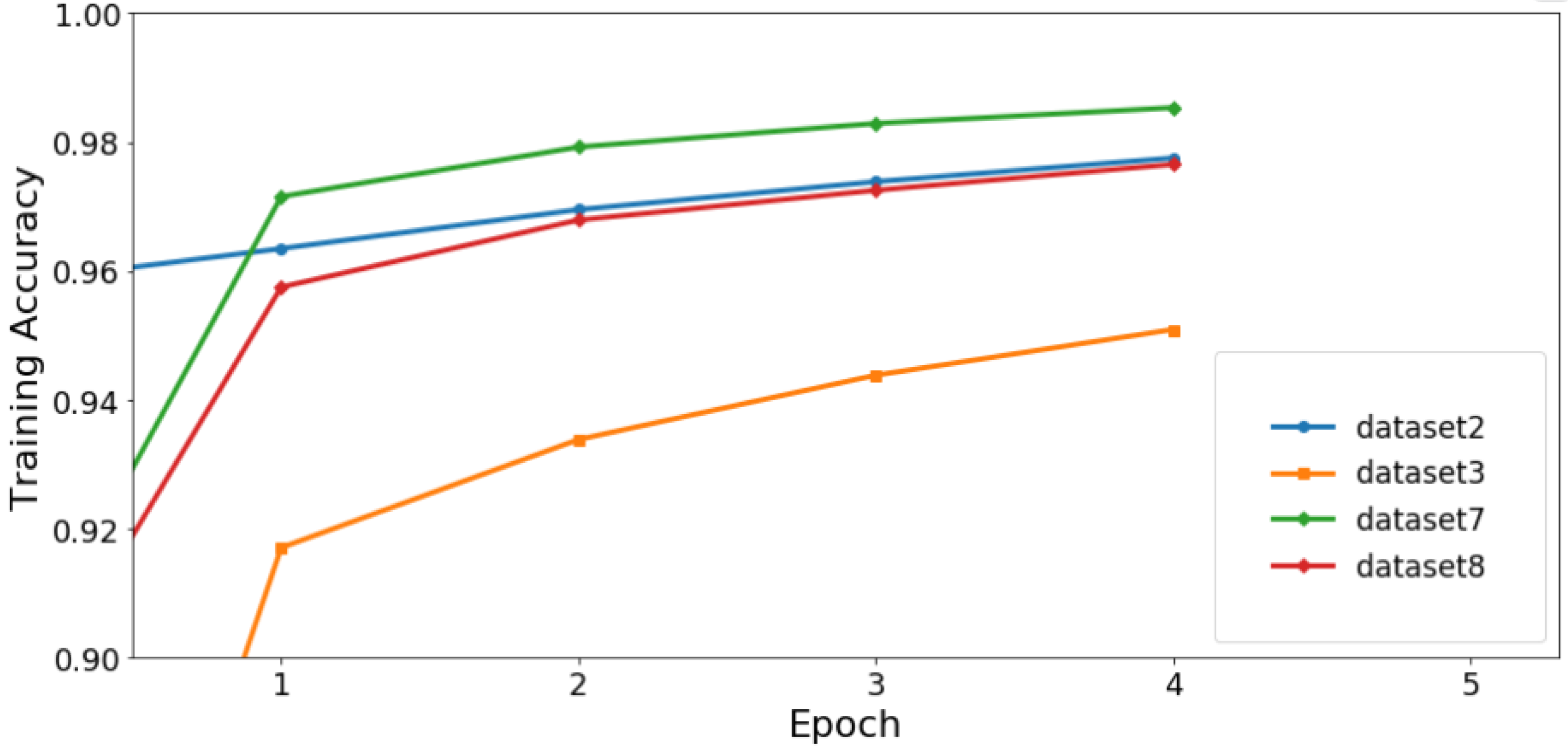
Table 2. Comparison with other datasets for testing accuracy and calculation time.

Trained Dataset	Training Accuracy	Validation Accuracy
Dataset 2	0.97	0.81
Dataset 3	0.95	0.81
Dataset 7	0.98	0.95
Dataset 8	0.97	0.93

compares the training and validation accuracy for several trained datasets. Dataset 8 outperforms dataset 2 with an training accuracy level of 97% and a validation accuracy level of 93%. Figure 9 and Figure 10 depicts a graphical representation of training and validation accuracy levels for various datasets.

Table 3. Comparison with other datasets for testing accuracy and calculation time.

Trained Dataset	Testing Accuracy	Calculation Time
Dataset 2	0.80	0.001
Dataset 3	0.82	0.002
Dataset 7	0.92	0.003
Dataset 8	0.91	0.002

, compares the testing accuracy and calculation time of different datasets.

Figure 9 compares the accuracy levels of different datasets based on training with 5 Epochs. Dataset 2 has a training accuracy level of 97%, whereas dataset 3 has a level of 94%. The training accuracy of four different datasets was tested, and their accuracy level was calculated. The highest training accuracy was observed for dataset 7 at 98%.

In Table 3, the results are based on the different trained datasets presented with testing accuracy and the calculated time that is estimated based on the training samples. Dataset 2 achieves a testing accuracy of 80% and a calculation time of 0.001, whereas dataset 8, which is the unseen dataset, presents a 91% testing accuracy level. Table 3 presents the training, testing accuracy, and calculation time.

To analyze the output matrices’ scores using the GTSRB dataset, Precision, Recall, and F1 Score are three metrics typically needed for a neural network model on a binary classification problem, in addition to classification accuracy. The accuracy determines how many positive class forecasts there are. Both positive samples in the dataset were used to create a recall prediction. F-Measure forecasts a single score that accounts for accuracy and recall in a single number.

$$Precision=\frac{True Positive}{True Positive+False Positive}$$

$$=\frac{True Psotive}{Total Predited Positive}$$

$$Recall=\frac{True Positive}{True Positive+False Negative}$$

$$=\frac{True Psotive}{Total Actual Positive}$$

$$F1 Score=2*\frac{Precision*Recall}{Precision+Recall}$$

Table 4. Performance metrics score with different sets of images.

Data	Precision	Recall	F1 Score	Support
Speed limit (20 km/h)	1.00	0.97	0.99	113
Speed limit (30 km/h)	1.00	0.99	0.99	926
Speed limit (50 km/h)	1.00	0.99	1.00	775
Speed limit (60 km/h)	0.99	0.99	0.99	506
Speed limit (70 km/h)	0.99	1.00	1.00	804
Speed limit (80 km/h)	1.00	1.00	1.00	321
End of Speed limit (80 km/h)	1.00	1.00	1.00	321
Speed limit (100 km/h)	1.00	1.00	1.00	214
Speed limit (120 km/h)	1.00	1.00	1.00	164
No passing	1.00	1.00	1.00	415
No passing for vechiles over 3.5 metric tons	0.99	1.00	0.99	479
Right-of-way at the next intersection	0.99	1.00	0.99	79
Priority road	1.00	0.99	0.99	487
Yield	0.99	0.99	0.99	110
Stop	1.00	1.00	1.00	112
No Vechicles	1.00	1.00	1.00	123
Vechiles over 3.5 metric tons prohibited	0.98	0.99	0.99	190
No entry	0.98	0.99	0.99	104
General caution	1.00	1.00	1.00	599
Dangerous curve to the left	1.00	1.00	1.00	198
Dangerous curve to the right	1.00	1.00	1.00	81
Double curve	1.00	0.98	0.99	204
Bumpy road	0.99	1.00	0.99	94
Slippery road	0.98	1.00	0.99	531
Road narrows on the right	0.99	1.00	0.99	173
Road work	1.00	1.00	1.00	295
Traffic signals	0.99	1.00	0.99	96
Pedestrians	1.00	1.00	1.00	274
Children crossing	1.00	0.98	0.99	172
Bicycles crossing	1.00	1.00	1.00	480
Beware of ice/snow	1.00	0.99	0.99	162
Wild animals crossing	1.00	1.00	1.00	87
End of all speed and passing limits	0.99	1.00	1.00	772
Turn right ahead	1.00	1.00	1.00	113
Turn left ahead	0.99	1.00	1.00	767
Ahead only	1.00	0.97	0.98	126
Go straight or right	1.00	0.99	0.99	90
Go straight or left	1.00	1.00	1.00	75
Keep right	0.99	0.98	0.99	731
Keep left	0.99	1.00	1.00	150
Roundabout mandatory	0.99	0.99	0.99	575
End of no passing	0.99	1.00	1.00	513
End of no passing by vechiles over 3.5 metric tons	0.99	0.99	0.99	544
Accuracy			1.00	14,628
macro avg	1.00	0.99	0.99	14,628
weighted avg	1.00	1.00	1.00	14,628

presents the performance metrics tested with different sets of sign classes and measured with precision-recall and F1 Scores. The support index is measured as the F1 Score reacting as balanced and imbalanced predictions.

In

Table 5. Accuracy level of different class labels.

Class_Label	Accuracy
Speed limit (20 km/h)	97.35
Speed limit (30 km/h)	99.03
Speed limit (50 km/h)	99.48
Speed limit (60 km/h)	99.41
Speed limit (70 km/h)	99.75
Speed limit (80 km/h)	99.88
End of speed limit (80 km/h)	100
Speed limit (100 km/h)	100
Speed limit (120 km/h)	100
No passing	100
No passing for vehicles over 3.5 metric tons	100
Right-of-way at the next intersection	100
Priority road	99.18
Yield	98.18
Stop	100
No vehicles	100
Vehicles over 3.5 metric tons prohibited	98.95
No entry	99.04
General caution	99.83
Dangerous curve to the left	96.97
Dangerous curve to the right	100
Double curve	98.04
Bumpy road	100
Slippery road	100
Road narrows on the right	100
Road work	100
Traffic signals	100
Pedestrians	100
Children crossing	98.26
Bicycles crossing	100
Beware of ice/snow	98.77
Wild animals crossing	100
End of all speed and passing limits	99.87
Turn right ahead	100
Turn left ahead	100
Ahead only	96.83
Go straight or right	98.89
Go straight or left	100
Keep right	98.36
Keep left	100
Roundabout mandatory	99.3
End of no passing	99.81
End of no passing by vehicles over 3.5 metric tons	99.45

the results are based on multiclass labels in the GTSRB dataset. For most of the traffic signs with noisy and unseen data of fast moving vehicles the images were used to exactly predict the content. The ELVD model predicted the speed limit of 60 km/h with a 99.41 accuracy level.

7.2. Predicting with One Image Dataset from Test Dataset

The prediction of particular images is conducted using the scores of forward passes of input images. Scores are given for images with 43 numbers of predictions for each class with only one class having a maximum value. The following table shows the predicting class id for model trained datasets.

Table 6. Comparison of datasets to predict an unknown dataset of different labels [2,25].

Trained Dataset	Predicted Label
Dataset 2	Speed limit (60 km/h)
Dataset 3	Speed limit (80 km/h)
Dataset 7	Speed limit (60 km/h)
Dataset 8	Speed limit (60 km/h)

compares the different datasets for trained and predicted models of particular unseen class labels. Figure 11 shows the unseen class labels and LHE, STD and Mean used to predict the content of labels.

7.3. Case Study: ELVD Based CNN

Due to several obstacles, including nonuniform lighting, motion blur, occlusion, and hard negative samples, detecting traffic signs is particularly difficult. Manual features, like HOG, that increase information of a typical hue or geometric shape sometimes fail in challenging circumstances. Nevertheless, CNNs are regarded as strong and effective in many applications, and some pertinent work based on CNNs has been conducted. We propose an ELVD-based CNN approach to guide traffic sign datasets with deep CNN for object classification. Our research reveals that drivers often read traffic signs from the top down and from left to right.

7.4. Pipeline Architecture

• Load The Data.
• Dataset Summary & Exploration.
• Data Preprocessing.
  • Shuffling.
  • Grayscaling.
  • Local Histogram Equalization.
  • Normalization.
• Design a Model Architecture.(ELVD with CNN).
  • LeNet-5.
  • GGNet.
  • DropoutNet.
• Model Training and Evaluation.
• Testing the Model Using the Test Set.
• Testing the Model on New Images.

7.5. Model Architecture: ELVD

In this phase, we will design and implement a deep learning model that uses our dataset and the GTSRD and TSRD datasets to learn to detect traffic signs. To categorize the images in this dataset, we will utilize convolutional neural networks combined with the ELVD model (Figure 12). Convolutional networks were chosen because they can identify visual patterns without much preprocessing straight from pixel images. They are automatically derived from data hierarchies of invariant properties at each layer. 1. We train the network on how frequently to update the weights by specifying a learning rate of 0.001. 2. We employ the Adaptive Moment Estimation (Adam) Algorithm to minimize the loss of function [46,47,48].

For each parameter, the Adam algorithm calculates adaptive learning rates. In addition to storing the average of the previous squared gradients with exponential distribution, for each parameter, the Adam algorithm calculates adaptive learning rates. The average of the consecutive squared gradients with an exponential distribution is further retained.

7.6. Model Training for ELVD

A significant issue with deep neural networks is overfitting. Dropout is a method for solving this issue. The basic concept is to randomly remove units and connections from the neural network while it is being trained. Units are prevented from co-adapting as a result. Dropout samples from an exponential range of several “thinned” networks are used during training. By utilizing a single thinned network with such a decreased weight at test time, it is simple to replicate the impact of averaging the predictions of all these thinned networks. This provides considerable gains over conventional regularization techniques and considerably lowers overfitting. To begin training the model, we will now pass the training data via the pipeline.

▪

We will vary up the training set before every epoch.

▪

We calculate the validation set’s accuracy and loss at the end of each period.

▪

We will retain the model after training as well.

▪

Low levels of accuracy on the training and validation sets indicate underfitting. Overfitting is implied when the validation set’s accuracy is low while the training set’s accuracy is high.

7.7. Model Testing for ELVD

The model correctly identified the “Speed limit” sign as such, but it appeared to be perplexed by the various speed restrictions. However, it accurately anticipated the final class. Each of the five new test photos had the correct class predicted by the VGGNet model resulting in 100% accuracy on the test. The model was 80% to 100% certain in every situation.

Table 7. Result of ELVD with different State-of-the-Art Techniques.

Model	No of Training Images	AUC (%)	(~Time)	Ap	mAp	Detection Rate
MCDNN [49]	2000	97.10	-	18.01	35.94	97.10
	4000	95.50	-	10.01	43.10	96.33
	6000	95.10	~460	13.11	35.20	96.88
	8000	96.89	~1133	13.33	38.80	97.10
Mask RCNN [50]	2000	97.35	~	11.45	34.88	96.22
	4000	97.42	~478	12.76	43.10	96.78
	6000	96.23	~1622	14.11	50.16	97.77
	8000	97.89	~1755	14.13	56.12	97.33
SVM [51]	2000	97.10	-	11.33	36.76	95.56
	4000	96.50	~466	11.07	47.21	95.77
	6000	96.45	~1622	14.02	52.66	95.89
	8000	97.76	~1655	14.01	59.91	96.32
HOG [52]	2000	95.21		11.01	36.89	96.43
	4000	96.22	~311	12.34	48.10	96.33
	6000	97.31	~1133	14.01	52.20	97.79
	8000	97.72	~1635	16.08	59.80	97.56
SSD [53]	2000	97.56	-	08.01	36.94	96.00
	4000	96.34	~462	10.01	48.26	9654
	6000	97.43	~1568	14.02	55.20	96.98
	8000	97.87	~1755	16.07	59.91	97.58
ELVD	2000	98.94	-	16.01	50.01	97.58
	4000	98.94	~151	16.03	52.02	98.89
	6000	98.89	~176	18.01	60.06	98.94
	8000	99.10	~184	19.23	67.76	99.10

presents the result of different training samples with different state-of-the-art techniques. Figure 13 shows the graphical analysis with AUC score of the comparison with other state-of-the-art techniques.

$$\mathrm{AP}={{\displaystyle \int }}_0^{1}p\left(r\right)dr$$

(8)

$$\mathrm{mAP}=\frac{1}{N}{\displaystyle \sum }_i^{N}A{P}_i$$

(9)

According to our tests, it is possible to obtain a high classification accuracy without making any adjustments. As a result, we only extracted the HOG feature from the input’s grayscale version to use an SVM to categorize the features in the image. We obtain the greatest accuracies of 99.10%, 98.89% and 98.94% for required, different and training images, respectively, using the same training technique as super class classification. MCDNN, requires a long period of time, whereas quick techniques like ELVD only require a few minutes.

7.8. Comparative Analysis with Different Models

Table 8. Comparative analysis with other Existing methods.

			Image Size Comparision
Dataset	Method	Detection Rate	mAP (Samll)	mAP (Middle)	mAP (Large)	Average Detection Time
GTSRB	LeNet	94	53.25	66.30	75.54	0.004
	VGGNet	95	46.66	51.45	60.21	0.003
	DropoutNet	96	28.56	42.20	44.56	0.002
	Faster R-CNN Resnet 50	93	46.25	58.30	65.25	0.002
	Faster R-CNN Resnet 101	92	53.50	86.95	86.65	0.003
	Faster R-CNN Inception V2	93	70.85	94.17	88.68	0.003
	Faster R-CNN Inception Resnet V2	96	56.80	86.08	88.53	0.003
	R-FCN Resnet 101	96	60.37	84.23	81.10	0.002
	SSD Mobilenet	97	26.25	66.72	79.26	0.002
	Proposed ELVD	98	47.88	80.25	82.65	0.001
TSRD	LeNet	93	55.30	68.22	82.87	0.005
	VGGNet	92	48.36	52.33	64.00	0.005
	DropoutNet	92	28.56	45.37	46.36	0.004
	Faster R-CNN Resnet 50		48.36	60.36	63.35	0.003
	Faster R-CNN Resnet 101	90	56.35	84.23	83.32	0.004
	Faster R-CNN Inception V2	89	68.30	92.36	89.36	0.004
	Faster R-CNN Inception Resnet V2	88	57.35	88.53	88.00	0.002
	R-FCN Resnet 101	90	60.02	84.10	81.26	0.002
	SSD Mobilenet	92	28.36	66.02	79.10	0.002
	Proposed ELVD	94	49.92	80.33	79.56	0.002

compare the different methods of State of Art Technique with detection rate and average detection time compared with LeNet, VGGNet and DropoutNet tested with GTSRB and TSRD. Our proposed model predicts the detection rate with high accuracy levels when comparing both datasets.

The mean Average Precision or mAP score is calculated by taking the mean AP over all classes and/or overall IoU thresholds, depending on different detection methods. Figure 14a shows a comparative analysis with other standard methods for the GTRSB dataset. Figure 14b describes the comparative analysis with other methods for the TSRD dataset.

7.9. Research Issues in ELVD Model

The process of creating a traffic sign detection system is demanding and difficult. There are a number of research factors that can contribute to the effectiveness of the GTSRB and TSRD dataset’s method of traffic sign identification and recognition. Each dataset of the GTSRB and TSDR scheme that the model conflicts with can be separated into the following research issues:

• Lighting

One of the key research problems interfering with the implementation of a GTSRB and TSDR system for the issues of uncertain lighting circumstances is the development of a GTSRB and TSDR framework. Different colors and information are used on road signals to aid in the interpretation of changes in lighting.

• Damaged Traffic Signs

Both the identification and identification steps of the process will be lost due to damaged and invisibly blocked traffic signs.

• Effects of Blurring and Fading

For a GTSRB and TSDR scheme, another key problem is the fading and blurring of traffic signs brought on by lighting during rain and snow. The aforementioned test circumstances will result in more false detections and poorer performance from the TSDR and GTSRB devices.

• Motion Artifacts

Moving vehicles can contribute to motion blur. Lower resolution cameras are subject to noisy or blurred images.

• Establishment of the Region

Different objects on the path that are detected cause an obstruction for the device, thus definitive traffic sign identification is not achieved. For example, advertising banners on the path, could cause inaccuracies in target area development.

• Poor Visibility

The main causes of low visibility are the shadows cast by other vehicles’ headlights. Rain, snow, and foggy conditions are other research factors that may reduce perception. These conditions may have unusual effects on the functioning of a GTSRB and TSDR system. The proposed ELVD model discovered that classification may be added on top of detection. In addition, developing a classification model is considerably quicker and easier, making it a useful strategy for grouping the discovered classes into multiple subclasses. The optimal balance between accuracy, detection time, and correctly classifying traffic sign images is achieved by our ELVD model.

8. Conclusions and Suggestions for Future Research

Deep learning has a number of advantages over conventional machine learning approaches in terms of revealing significant attributes in a high-dimensional database. Recently, CNNs have been associated with great developments in processing text, speech, images, videos, and other applications. In the “Pedestrian” sign images, there is a triangle sign with a shape inside it, and the pictures copyrights add some noise to the image, reducing the main characteristic of the ELVD model’s confidence significantly. The model was able to predict the real quality, albeit with 80% confidence. To conclude, the ELVD model accurately predicted samples including noisy and foggy images; it predicted the exact content using ensemble-based VGGNet, LeNet and DropoutNet for removal of unnecessary details. For each of the five new test images, the ensemble-based LeNet and VGGNet (ELVD) model was able to predict the appropriate class with a 100% test accuracy. The model was extremely confident in each scenario (80–100%). ELVD achieved a high accuracy rate with VGGNet. The model saturated after about 10 epochs, thus it may limit the number of epochs to save some computing resources. Other preprocessing methods like a YOLO-based Ensemble approach can be used to further enhance the model to improve the image recognition accuracy under more extreme conditions and predict the label with more accuracy.