1. Introduction
With their expansion on the “internet-scale”, the complexity of networks also increases. In order to use network resources more effectively, it is necessary to acquire the changes in quality and performance parameters of communication links conveniently and accurately. The packet loss rate is an important performance indicator to measure the quality of communication links. Furthermore, timely and accurate prediction plays an important role in cross-layer optimization [
1]. Based on whether the time-variance of the communication link is considered or not, the prediction methods are classified into stationary and non-stationary types. At present, most studies have only focused on stationary communication links. For example, Refs. [
2,
3,
4] predicted the distribution of end-to-end link delays through the mathematical modeling of links. Refs. [
5,
6,
7,
8] assumed that links are stationary and subject to a certain distribution and established a statistical model based on this assumption. Based on the results of end-to-end packet loss rate measurements or simulations, the model parameters are estimated by the high-order moment, least square, and maximum likelihood methods to obtain the probability distribution of packet loss rate compliance. Ref. [
9] analyzed the factors affecting the packet loss rate in transmission control protocol (TCP). The acknowledge (ACK)-to-packet ratio was selected as a statistic of the functional relationship between fitting and packet loss rate. Although this method has obtained high accuracy in simulation experiments, it was proven that the actual data fitting effect is not satisfactory in the experimental platform built in the current paper. In Ref. [
10], in the media access control (MAC) layer, a non-flat, hidden Markov chain model based on the carrier sense multiple access with collision avoid (CSMA/CA) mechanism was proposed to predict the packet loss rate. The model has three state variables, representing the number of nodes competing for the same channel in the topology, the number of nodes currently competing for the channel, and the number of nodes successfully obtaining the channel, respectively. According to this, the state space was divided and the non-stationary Markov chain model was established. To reduce the complexity of the estimation algorithm of the packet loss rate, Ref. [
11] theoretically analyzed the factors affecting the packet loss rate in a tree topology, and provided an unbiased estimation of the packet loss rate in various topologies. Ref. [
12] modeled the packet loss rate series as a time series, and the autoregressive integrated moving average model (ARIMA) was used to predict the packet loss rate. Using historical experimental data as input, the average fluctuation in historical data was used to predict the packet loss rate. The ARIMA model is very simple and does not require any external parameters, but it is still very limited because it can only capture linear relationships and requires multiple differences in the input data to obtain a stationary sequence.
However, the high suddenness of actual network traffic makes the state of links change frequently. Therefore, the prediction results on the premise of stationary networks cannot reflect the time-varying characteristics of network link parameters [
13,
14]. The non-stationary communication link parameter prediction method considers that the link state is time-varying and can track the change in link parameters over time. The difficulty of this problem is that the stationary link prediction method of traditional regression analysis always produces large errors due to the constant fluctuation in the link state, while the prediction method based on deep learning is usually of high complexity, cannot guarantee the timeliness of the algorithm, and there is still a lack of an effective solution [
15]. Ref. [
16] proposed a method to predict the packet loss rate of time-varying networks through artificial neural networks, but there was no unified and complete theoretical guidance for the selection of a network structure, which can only be selected by experience. In Ref. [
17], a low-order linear regression method was used to predict the packet loss rate of time-varying networks. Nevertheless, the selection of regression variables and the corresponding relationship is an empirical prediction. In some cases, the method of low-order linear regression is less accurate. Ref. [
18] proposed a non-stationary link delay prediction method, which uses the sequential Monte Carlo method to track non-stationary network link behavior and estimate the time-varying characteristics of link delay. The sequential Monte Carlo method is an estimation method based on Bayesian filtering, which needs to estimate the prior information of the model; however, it is generally difficult to obtain accurate prior information, which will lead to the degradation of the estimation performance.
In this study, we propose a prediction of the packet loss rate of non-stationary links. The packet loss rate of network links is time-varying and can be expressed as a non-stationary time sequence. To solve this problem, a TVAR model is established to analyze, process, and predict the packet loss rate of non-stationary links. The characteristics of this model are to characterize non-stationary time sequences by a time-varying coefficient and a moving average. Therefore, it is of great significance to study the estimation algorithm of time-varying coefficients [
19,
20]. In this study, the maximum entropy principle and the least square method are used to estimate the packet loss rate, and then the packet loss rate is predicted according to the time-varying coefficient estimation results. The main contributions of this paper can be summarized as follows:
In this paper, we analyze the TVAR sequence and transform the estimation problem of the time-varying coefficient into a constrained optimization based on the principle of maximum entropy. By solving the problem, we obtain the estimated value of the time-varying coefficient. Based on this, we provide the one-step prediction and multi-step prediction algorithms of the TVAR sequence.
This paper analyzes the packet loss problem of a non-stationary network, defines the packet loss rate of a time window by establishing the network model and introducing the concept of a time window, and defines the packet loss rate of a non-stationary network based on this.
In this paper, the Gilbert–Elliot model is improved to better reflect the time-varying characteristics of non-stationary networks and the time-varying packet loss sequence is generated as a link model, which is used to verify the validity of the TVAR sequence prediction method.
In this paper, a small wireless multi-hop network experiment platform is built in reality, and the prediction effect of two common prediction methods is compared with that of the TVAR sequence prediction method. It is found that the TVAR sequence prediction method can obtain higher prediction accuracy with lower time complexity.
Next, we will list some common symbols and their meanings in this article, as shown in
Table 1:
3. Mathematical Modeling
Similar to most research [
29,
30,
31,
32,
33,
34], in this study, source nodes and multiple target nodes are modeled as graph theoretic models,
.
T is a logical tree, representing the set of nodes,
V, and link,
E.
V is a set of nodes, which consists of source node
S, destination node
D, and an internal node. The path from source node
S to destination node
Di is represented as
P(
S,
Di), and the set of links on
P(
S,
Di) is represented as {
ei,1,
ei,2 ei,K}. The network topology model is shown in
Figure 1.
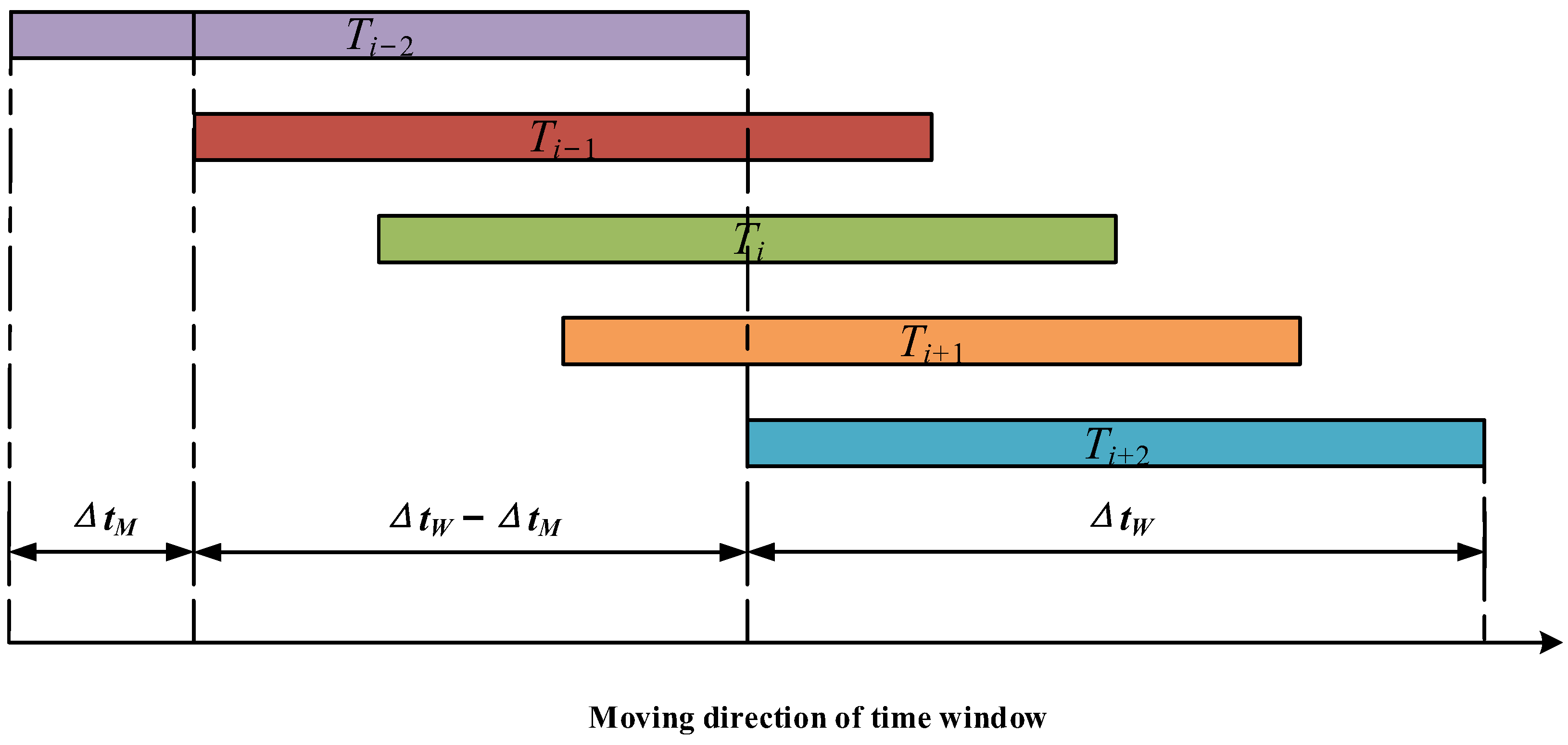
In order to represent the time-varying characteristics of the network link packet loss, this study introduces the idea of a sliding time window to redefine the time-varying packet loss rate of the link. First, the measurement cycle is divided into smaller periods; each period is called a time window. The packet loss rate of the link within the time window changes relatively smoothly, which can be considered quasi-stationary [
15]. The sliding process of the time window is shown in
Figure 2.
In
Figure 2,
is the sliding step of the time window and
is the length of the time window. In order to ensure the continuity of the estimation results,
and
should meet the following conditions:
. The overlap length of adjacent time windows is
, and
s is defined to represent the overlap ratio between time windows
:
The larger the value of s, the more overlapped the time window and the smoother the packet loss rate curve of the time window. The relationship between the time window length,
, the time window overlap ratio,
s, and the number of time windows,
N, can be expressed by the following formula:
where, [·] indicates downward rounding. It can be seen that the larger
s is, the larger
N is, the smoother the transition of the time window packet loss rate will be, and the lower the probability of a sudden change in the packet loss rate during the statistical process is. In this study, the time-window packet loss rate of link
P(
S,
Di) is defined by the following form:
where
k is the serial number of the time window and
indicates the number of packets sent by node
s to
Di within the time period
. The number of these packets received by
Di is
.
At present, the change in packet loss rate with the time window can be characterized according to the definition of the packet loss rate of the time window. However, the packet loss rate of the time window can only reflect the average packet loss rate in all time windows and cannot reflect the change in the packet loss rate in a single time window. The inverse distance squared weighting (IDSW) algorithm was used to determine the value of the time-varying packet loss ratio (
PLRt) at any time in response to the problem of an imprecise time-window packet loss ratio [
35,
36]. The algorithm flow is shown in Algorithm 2.
| Algorithm 2 Inverse Distance Square Weighting |
| Input: n, t, p1, p2, …, pn, t1, t2, …, tn; |
| Output: PLRt; |
| 1: | ifn = 1 |
| 2: | then return p1; |
| 3: | end if |
| 4: | ift − ti = 0 |
| 5: | then return pi; |
| 6: | else |
| 7: | fori ← 1 to n |
| 8: | wi ← 1/(t − ti)2; |
| 9: | end for |
| 10: | end if |
| 11: | w ← ∑wi; |
| 12: | PLRt ← (1/w)∑pi wi; |
n is the number of time windows including time t, pi is the packet loss rate of the time window whose serial number is i, and ti is the midpoint of the time window whose serial number is i. The increase in n indicates that the value of the time-varying packet loss rate of the link at time t has more times of repeated estimation; hence, the final estimated value at this time is more accurate. On the other hand, since the time-varying packet loss rate in each time window is estimated independently, the increase in n will increase the computation amount of the whole algorithm.
4. Model Simulation
To verify the correctness of the prediction of the link packet loss rate in a non-stationary network by using the TVAR sequence method, it is necessary to contruct a simulation environment similar to the real network. First, a network topology for simulation was constructed, as shown in
Figure 3.
In the network topology shown in
Figure 3, there are eight nodes and seven links. Node
S, as the source node, sends packets to destination nodes
D4,
D5, and
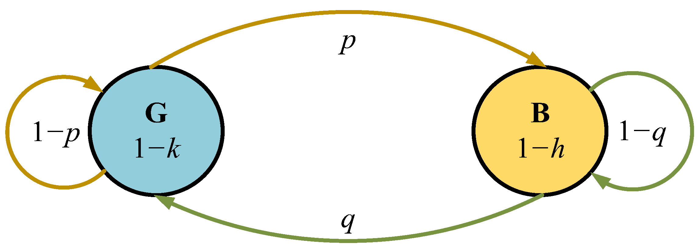
D6. In order to simulate the packet loss rate for each time window in the path from the source node to the destination node, the link needs to be modeled. The model used in this study was improved based on the Gilbert–Elliot model. The Gilbert–Elliot model uses first-order Markov chains to simulate packet loss events in non-stationary networks, and its main advantage lies in considering the dependence between packet loss events [
37,
38,
39,
40].
As shown in
Figure 4, the link in the Gilbert–Elliot model has two states, namely “G(good)” and “B(bad)”. In the G state, the packet has a probability of 1−
k to be lost, while in the B state, the packet has a probability of 1−
h to be lost. The probability transition matrix is shown below:
In this study, based on the Gilbert–Elliot model, a “medium” state was added between “good” and “bad” link states. In order to better reflect the time-varying characteristics of links, the packet loss rate of each state is no longer set as a fixed value, but is set as a random variable that follows a Gaussian distribution.
As shown in
Figure 5,
P1,
P2, and
P3 are the packet loss rates of the three states, which meet the following conditions:
In order for
Pi to satisfy
, according to the 3σ principle of normal distribution, the variance should also satisfy the following relation:
In the simulation, the network traffic consisted of 200,000 UDP packets, where the size of each packet was 1000 Bytes, the transmission rate was 0.1 MBps, the length of the time window was 10 s, the step of the time window was 5 s, and the measurement period was 2000 s, with 200 windows in total.
Table 2 lists the link parameters.
According to the link model and parameter settings, the boxplot of the packet loss rate from the source node to the destination node and its probability distribution function image were obtained and are shown in
Figure 6.
In the above figure, path
i represents the path from source node S to destination node
Di, that is, P(
S,
Di) in
Figure 3, (i = 1, 3, 4, 5, 6). The boxplot shows that almost all links have no abnormal packet loss rates. The median packet loss rates of path 1 and path 3 are low, concentrated, and fluctuate slightly. The packet loss rates of path 4, path 5, and path 6 are similar. Compared with path 1 and path 3, the packet loss rates of path 4, path 5, and path 6 have a higher median, a more dispersed distribution, and a greater fluctuation. From the perspective of the distribution function, the packet loss rate curves of path 1, path 3, and path 4 are similar in shape. The head and tail of the curve are gentle, while the middle of the curve is steep, which is close to the distribution function of normal distribution. Combined with the selection of the model and the setting of parameters, the experimental results can be explained. Whether the link quality is good or bad, the possibility of packet loss increases with each additional hop, which is the reason why the packet loss rates of path 6, path 5, and path 4 are generally higher than those of path 3 and path 1. As can be seen from
Table 1, the variance parameters of the simulation experiment model are set to be relatively small, which makes the packet loss rate distribution more concentrated. Since packets from S to D
6, D
5, and D
4 all pass through P(S, D
0) and P(S, D
1), i.e., path 6, path 5, and path 4 share most links, their packet loss rates are similar. Finally, since the model assumes that the transfer probability of link mass is subject to a normal distribution and each link mass corresponds to a fixed packet loss probability, the distribution of the packet loss rate is close to a normal distribution.
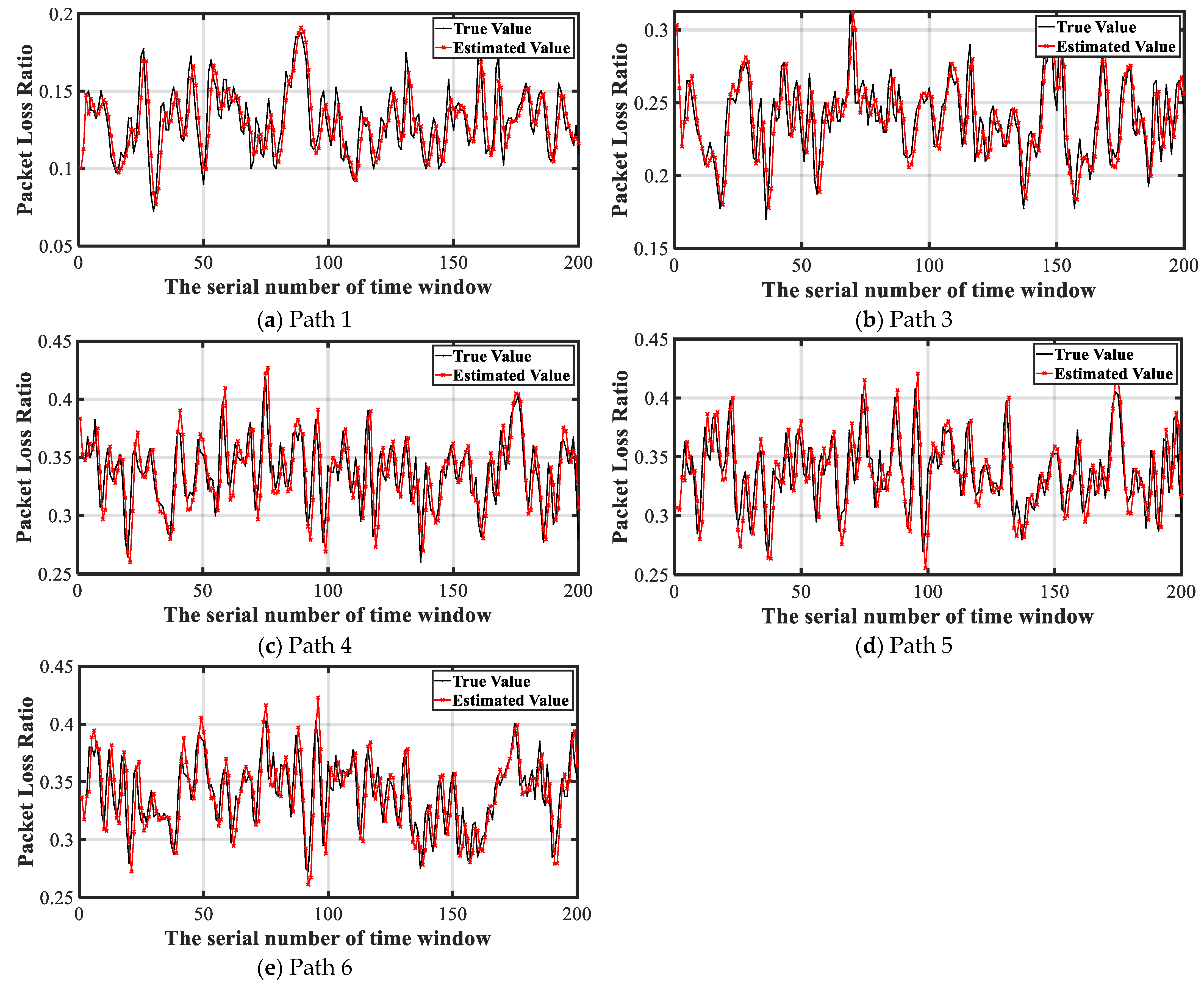
Next, this paper will predict the packet loss rate of each time window of path 1, path 3, path 4, path 5, and path 6 based on a TVAR sequence.
Figure 7 shows the curves of the predicted value and actual packet loss rate of each path in the network simulation model.
As can be seen from the real value curve of the link packet loss rate, the packet loss rate of a one-hop link is distributed in (0.05,0.20), that of a two-hop link in (0.15,0.35), and that of a three-hop link in (0.25,0.45). The distribution of the packet loss rate of the link is relatively concentrated, with almost no outliers, and the mean value increases with the increase in the hop number, which is consistent with the results reflected in
Figure 7. The predicted value curve of the link packet loss rate was predicted according to the TVAR sequence method. On the whole, the predicted value curve is close to the real value curve and truly reflects the packet loss status of the link. However, the TVAR sequence needs to take the current statistical packet loss rate as the input of the sequence and update the parameters of the sequence after a series of operations, which leads to a lag in the prediction of the TVAR sequence. It can also be seen from the figure that the predicted value is usually close to the real value of the previous time window, which is also the main source of the prediction error using the TVAR sequence. Therefore, when the time series continuously has a large jump, the prediction of the TVAR series will inevitably produce some errors. However, if the time series is relatively stable, the prediction accuracy of the TVAR series will be further improved.
In order to quantify the predictive performance of the TVAR sequence method, the root mean square error (
RMSE) was used to calculate the overall deviation between the predicted value and the actual value of the link packet loss rate [
41,
42]:
The RMSE describes the dispersion degree of the sample by calculating the standard deviation of the residual. The smaller the RMSE is, the more accurate the predicted result is. The RMSE of each path was calculated and the results are shown in
Table 3.
As can be seen from
Table 3, in a multi-hop non-stationary network, the packet loss rate prediction method based on the TVAR sequence has relatively good prediction accuracy for each link. In addition, the prediction error jitter between links is small.
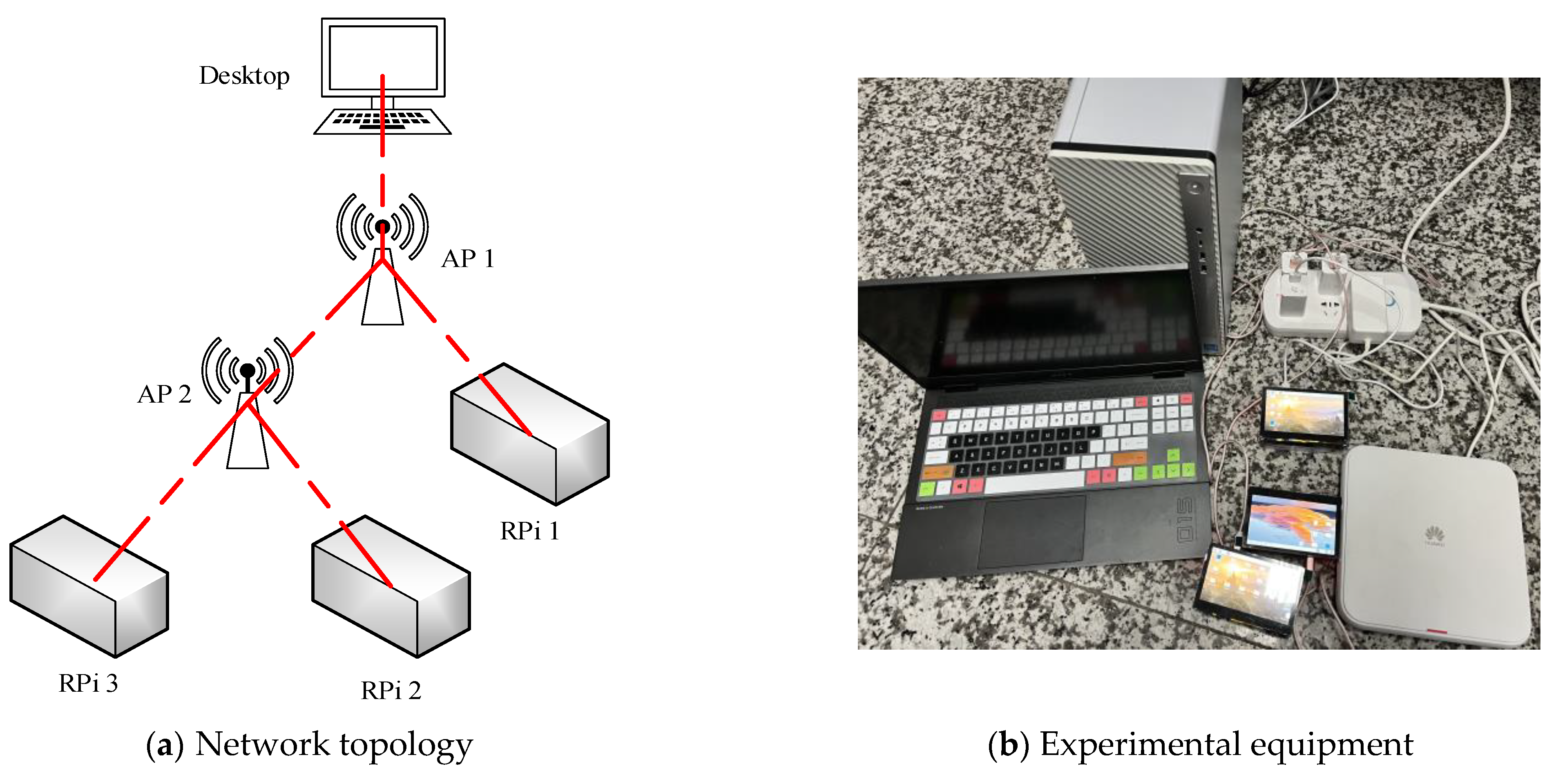
5. Experimental Verification
In order to verify the wide applicability of the packet loss rate prediction scheme based on the TVAR sequence, a small wireless multi-hop network experiment platform was built, whose network extension is shown in
Figure 8.
The experimental equipment included a desktop computer as the sender, an enterprise router as the forwarding node, a laptop computer sharing the network as a second forwarding node after connecting to the router, and three raspberry pis as the receivers.
Table 4,
Table 5,
Table 6 and
Table 7 list the details of all experimental devices.
The experimental platform was deployed in an office. Besides the small wireless network set up for the experiment, there were more than 20 other wireless networks for other students and teachers to use. These users caused unpredictable interference to the communication link set up in the experiment. An overhead view of the office is shown in
Figure 9.
Although raspberry pi (RPi) does not process information as fast or store it as a desktop computer, tests were conducted before the experiment to ensure that each device did not exceed its computing or storage limits during the experiment.
The NACK-Oriented Reliable Multicast (NORM) protocol was used to communicate between nodes. NORM is a reliable multicast transmission protocol which combines erasure codes and the negative acknowledgment (NACK) mechanism in user datagram protocol (UDP) to realize the reliable end-to-end file transmission function [
43]. The NORM protocol uses NACK for error control. If the receiver detects a packet loss, it waits for a random time based on the group round trip time (GRTT) [
44]. Within the random waiting period, if the receiving end receives a NACK from another group member, it will delete the same content in its own NACK to avoid the “feedback storm” of NACK. When the sender receives a NACK, the sender starts the repair program and enters the aggregation phase. At this time, the sender continues to receive NACK messages. After the aggregation stage, the sender retransmits the lost data block according to the collected NACK information and enters the backoff stage. After entering the backoff stage, the sender will not receive the NACK information anymore, but will directly discard the received NACK to avoid the overlap between the retransmitted data block and the new request arriving at the NACK [
45].
The packet loss rate of the time window was redefined according to the characteristics of the NORM protocol, such as sending information in the unit of data blocks and NACK information being discarded because the receiver was in the backoff stage.
where
represents the number of segments sent by the sender time-window with serial number
k, but these segments may not all be received by the receiver.
represents the number of lost segments requested to be retransmitted in the NACK received by the sender in the time window with serial number j.
Figure 10 shows the process of the sender sending segments in the time window with serial number k and receiving NACK due to segment loss. When calculating the packet loss rate in the time window, only
is included in the packet loss, while
is discarded. The IDSW algorithm is still used to define the time-varying packet loss rate (
PLRt).
The sending file consists of 2500 blocks, and each block consists of 32 segments with a size of 1056 Bytes. The sending rate is 0.1 MBps, the length of the time window is 10 s, and the step of the time window was 5 s. The rest use the default configuration of the NORM protocol.
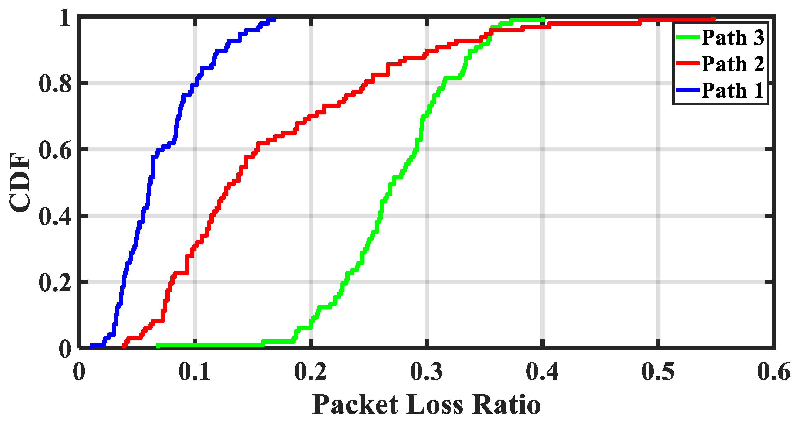
Firstly, according to the experimental data obtained in the above configuration, the probability distribution function of the packet loss rate of the three links between the sender and the three receivers is shown in
Figure 11.
The distributions of Path 1, Path 2, and Path 3 indicate the three links between the sender and the receiver RPi 1, Rpi 2, and Rpi 3. As shown in
Figure 9, Path 1 has only two hops and a short link. Therefore, the packet loss rate of Path 1 is concentrated in a relatively low range. As Path 2 and Path 3 have three hops and long links, the packet loss rate is concentrated in a high range. On the day of the experiment, more people in the office were located in the north, resulting in greater jitter on the link of Path 2 than that of Path 3.
Next, this paper will predict the packet loss rate of Path 1, Path 2, and Path 3 based on the TVAR sequence.
Figure 12 shows the bar graph of packet loss rate prediction error of each link.
Firstly, it can be seen from the packet loss rate curve that compared with the simulation model, the packet loss rate fluctuates more in the wireless network built in the real environment. Secondly, the packet loss rate increases significantly after the second forwarding, which may be due to the large performance gap between the two forwarding nodes in the network, one of which is an enterprise class router and the other is a mobile hotspot of a laptop. By using devices with different performances as forwarding nodes, the link in the experiment has more time-varying characteristics than that in the simulation. It can be seen from the error bars that when the packet loss curve is relatively stable, the error generated by the TVAR prediction method is small. However, when the packet loss rate fluctuates greatly, the TVAR prediction method cannot obtain accurate results every time, which is similar to the results of the simulation.
To further evaluate the performance of the TVAR sequence prediction method, it is necessary to compare it with some commonly used methods. The first prediction method we chose for comparison was the ARMA sequence. First, the packet loss rate sequence can pass the unit root test by difference. Then, we calculated the optimal order of ARMA using the Akakike information quantity criterion and we took the ARMA model obtained at this time as the first prediction method for comparison.
The second method used for comparison is the long short-term memory (LSTM) based on deep learning method. We used 70% of the data as a training set to train the network. After network convergence, we adjusted the parameters to achieve the best effect.
Figure 13 shows the prediction results and prediction errors of the three prediction methods.
According to the results shown in
Figure 13a–c, it can be seen that whether the network fluctuation is large or small, the prediction curve of the ARMA sequence has small fluctuations on the whole, so the accuracy is often low in the environment of drastic network changes. The LSTM network has a high accuracy in predicting the dataset used in the training, and sometimes can almost coincide with the real value curve, but it does not perform well for the test dataset, although we have tried to adjust the model parameters to the best. There are two possible reasons for this situation: the input information to the model is only the previous packet loss rate information, which limits the upper limit of the model, or the dataset used for training is not big enough, so the model cannot learn the real characteristics of the packet loss rate. As the model parameters need to be updated according to the packet loss rate of the current and past time windows, the packet loss rate prediction of the TVAR sequence has some lag. However, on the whole, the TVAR sequence can still accurately predict the packet loss rate in most time windows. The results in
Figure 13d show that in the wireless multi-hop network built in this paper, the prediction results of the TVAR sequence are not much different from those of the ARMA sequence and the LSTM network in the link with low fluctuation. However, the prediction accuracy of the packet loss rate of the TVAR sequence is higher than that of the ARMA sequence and the LSTM network in the highly fluctuating links. From the perspective of average error, if RMSE is taken as the error index, the prediction error of the TVAR sequence is reduced by 24.67% compared with the ARMA sequence and 23.28% compared with the LSTM network.


