Underwater Acoustic Target Recognition Based on Data Augmentation and Residual CNN

Abstract

In the field of underwater acoustic recognition, machine learning methods rely on a large number of datasets to achieve high accuracy, while the actual collected signal samples are often very scarce, which has a great impact on the recognition performance. This paper presents a recognition method of an underwater acoustic target by the data augmentation technique and the residual convolutional neural network (CNN) model, which is used to expand training samples to improve recognition performance. As a representative model in residual CNN, the ResNet18 model is used for recognition. The whole process mainly includes mel-frequency cepstral coefficient (MFCC) feature extraction, data augmentation processing, and ResNet18 model recognition. On the base of the traditional data augmentation, this study used the deep convolutional generative adversarial network (DCGAN) model to realize the expansion of underwater acoustic samples and compared the recognition performance of support vector machine (SVM), common CNN, VGG19, and ResNet18. The recognition results of the MFCC, constant Q transform (CQT), and low-frequency analyzer and recorder (LOFAR) spectrum were also analyzed and compared. Experimental results showed that the recognition accuracy of the MFCC feature was better than that of other features at the same method, and using the data augmentation method could obviously improve the recognition performance. Moreover, the recognition performance of ResNet18 using data enhancement technology was better than that of other models, which was due to the combination of the data expansion advantage of data augmentation technology and the deep feature extracting ability of the residual CNN model. In addition, although this method was used for ship recognition in this paper, it is not limited to this. This method is also applicable to other target voice recognition, such as natural sound and underwater voice biometrics.

1. Introduction

In the underwater environment, the target recognition is of great significance for ocean development and national defense security, and it has become the top priority in the field of underwater acoustics. Automatic underwater target recognition mainly includes feature extraction and classifier construction. With the development of sensors and intelligent information, traditional methods have gradually failed to meet the intelligent development requirements of underwater detection information processing. In recent years, machine learning technology, which has been so popular in the computer field, provides theoretical support for the intellectualization of underwater target recognition. Kamal et al. proposed the deep brief network (DBN) model to recognize underwater acoustic signals, realizing the signal recognition without labels [1]. Shamir et al. proposed a machine learning model in order to realize automatic recognition of various whales with the input of the acoustic features of whales [2]. Yue et al. compared support vector machine (SVM), DBN, and convolutional neural network (CNN) models to achieve effective recognition of ship target acoustic signals [3]. Yu et al. constructed various machine learning methods to detect the phonation of the North Atlantic right whale and reached the conclusion that the CNN could greatly improve the accuracy [4]. Mishachandar et al. effectively recognized manmade sounds, natural sounds, and marine animal sounds through a CNN model [5]. Song et al. used CNN to effectively classify underwater noise under different SNRs, and the recognition performance was better than that of SVM [6]. Yang et al. used a deep CNN model to realize ship target recognition by extracting the correlation information between multiple attributes [7]. Escobar-Amado et al. extracted the regions of interest of bearded seals in the spectrum and realized the effective classification of bearded seal sounds using CNN [8]. Luo et al. proposed a local energy normalization method for inputting the underwater sound data spectra of different lengths and applied CNN to the effective detection of the toothed whale echolocation sound [9].

The method proposed in this paper used the CNN classification model. CNN has been widely used in image classification, speech recognition, and other fields. In 2012, Krizhevsky et al. proposed the AlexNet model [10], which won the first place in the ImageNet competition and made great contributions in the field of computer vision. In 2014, Simonyan et al. proposed the VGG19 model and evaluated the image recognition performance after increasing the depth of the network [11]. Since then, a large number of excellent models have gradually emerged, such as ZFNet [12], GoogLeNet [13], Inception-Residual Net [14], SENet [15], etc.

As the depth and complexity of machine learning models increase, the requirement for the amount of data has also been increasing. Only through the massive labeled data training model can we achieve good recognition effect. In reality, the sample data of underwater acoustic sensitive targets are relatively scarce, which limits the recognition accuracy of machine learning. To increase the sample size required for machine learning training, data augmentation methods [16,17] have been gradually applied. The traditional data augmentation technology generally adds the transformation of geometry and color space to expand training samples. However, the training performance after the data expansion is limited due to the fact that the traditional data augmentation technology cannot obtain substantially generated samples. To avoid the limitations of traditional data augmentation technology, Goodflow et al. designed a generative adversarial network (GAN) [18]. Through the adversary training of generators and discriminators, the sample according to the distribution of true sample can be generated. Yang used low-resolution GAN to obtain samples based on various backgrounds [19]. Deep convolutional GAN (DCGAN) combines CNN with GAN to enhance the stability [20]. GAN can also be improved to a conditional model, namely, conditional GAN (CGAN) [21].

In the actual underwater environment, the acquisition of signal samples is often very difficult, which poses a great challenge to recognition. In this paper, a recognition method suitable for a small number of samples of underwater acoustic signal was proposed. The mel-frequency cepstral coefficient (MFCC) was extracted as the input feature. Traditional data augmentation technology and the DCGAN model were used to realize the expansion of samples. Residual CNN was designed as the classification model. The overall flowchart of this paper is shown in Figure 1.

2. MFCC

The MFCC, which was proposed based on the characteristics of the human ear, is a widely used feature in speech recognition. Given the particularity of the human ear structure, the listener can automatically separate the low- and high-frequency segments of audio, in which the low-frequency segment identifies its characteristics. On this basis, the characteristics of the human ear can be simulated, and effective spectrum features can be extracted (i.e., convert the spectrum into mel spectrum) by setting denser filters in the low-frequency segment and fewer filters in the high-frequency segment. Cepstrum is used in log functions to transform multiplicative signals into additive signals to reflect the low-frequency envelope spectrum characteristics and high-frequency detail features. Through cepstrum analysis of the mel spectrum, the MFCC can be obtained and used in underwater target recognition [22].

Figure 2 shows the MFCC feature extraction process, which was mainly composed of preprocessing, fast Fourier transform (FFT), mel filtering, and discrete cosine transform (DCT).

The preprocessing included pre-emphasis, framing, and windowing. Pre-emphasis enabled the spectrum of the signal to be gentler by raising the spectrum of the high-frequency segment. Framing divided the signal into several short-term signals in which the signal could be regarded as a stationary process. In the process of framing, overlapping segmentation was generally adopted to make the frame to frame excessively smooth. Windowing reduced the truncation effect of the signal. Thus, the signal and the window function were set as $s(n)$ and $w(n)$, respectively. The signal obtained after windowing is as follows:

$$s^{\prime }(n)=s(n)w(n),0\le n\le N-1,$$

(1)

where $N$ is the number of samples, and $w(n)$ is the Hamming window.

After preprocessing, FFT was implemented on all frames. The discrete spectrum $S_a^{\prime }(k)$ of the signal can be expressed as

$$S_a^{\prime }(k)={\displaystyle \sum _{n=0}^{N-1}{s}^{\prime }(n)}{e}^{-j2\pi k/N},0\le k\le N.$$

(2)

The spectrum was then filtered through a group of triangular bandpass filters to obtain mel filters. Moreover, M filters exist, and $f(m)$ represents the center frequency, of which $m=1,2,\cdots ,M$. The triangular filter is obtained as follows:

$$H_m(k)=\{\begin{array}{ll}0\hfill & ,k<f(m-1)\hfill \\ \frac{2(k-f(m-1))}{(f(m+1)-f(m-1))(f(m)-f(m-1))}\hfill & ,f(m-1)\le k\le f(m)\hfill \\ \frac{2(f(m-1)-k)}{(f(m+1)-f(m-1))(f(m)-f(m-1))}\hfill & ,f(m)\le k\le f(m+1)\hfill \\ 0\hfill & ,k>f(m+1)\hfill \end{array}.$$

(3)

The logarithmic energy by the filter is obtained as follows:

$$S^{*}(m)=\ln ({\displaystyle \sum _{k=0}^{N-1}\left|S_a^{\prime }(k)\right|H_m(k)}),0\le m\le M.$$

(4)

DCT is performed to calculate M logarithmic energies to obtain the MFCC of order L (L = 12–16); the formula for DCT is

$$C_n={\displaystyle \sum _{m=0}^{N-1}{S}_m^{*}\cos \frac{n*(m-0.5)*\pi }{M}},n=1,2,\cdots ,L.$$

(5)

In practical application, the cepstrum difference parameter (delta cepstrum) is calculated following the value of L MFCC cepstrum coefficients, which is expressed as

$$d_n=\{\begin{array}{ll}{C}_{n+1}-C_n\hfill & ,n<K\hfill \\ \frac{{\displaystyle \sum _{k=1}^{K}k(C_{n+k}-C_{n-k})}}{\sqrt{2{\displaystyle \sum _{k=1}^K{k}^2}}}\hfill & ,else\hfill \\ C_n-C_{n-1}\hfill & ,n\ge L-K\hfill \end{array},$$

(6)

where d represents the nth first-order difference result; $C_n$ represents the nth cepstrum coefficient calculated by Formula (5); L represents the order when calculating the MFCC; and K stands for the time difference of the first-order derivative, which is set at 1 or 2. The second-order difference result could be obtained when the calculation result was brought into Formula (6).

Generally, the MFCC and the first- and second-order cepstrum difference parameters were combined as the characteristic of the signal.

3. Data Augmentation

Machine learning methods need a mass of data driven to realize excellent recognition accuracy. In the scene of a small number of samples, the amount of the training set can be increased by the data augmentation technology. On the basis of converting the underwater acoustic data into images, the traditional data augmentation method and DCGAN can be used to expand the underwater acoustic data.

3.1. Traditional Methods

(1) In this paper, the contrast ranges of the adjusted images were set to be 0.1–0.9, 0.2–0.8, and 0.3–0.7. Three generated images can be obtained from the original signal diagram by adjusting the contrast.

(2) The horizontal and vertical zoom scope of the image was set to 0.9–1.1, and the translation scope was set to −30 to 30 pixels.

3.2. DCGAN

The GAN contains generation and discrimination networks [23]. In the training process, the generation network was used to produce simulation samples, and the discrimination network evaluated the facticity of the data. The two networks were trained together by confrontation to realize the optimum effect of sample expansion. After the training, only the generation network was reserved for the sample generation.

The DCGAN was derived from the GAN model. It combined CNN with a basic GAN, and generator and discriminator were applied to deep CNN. The DCGAN improved the stability of the basic model and the quality of generated results. Its discriminator and generator frameworks are shown in Figure 3 and Figure 4, respectively. The DCGAN had the following characteristics: It removed the pooling layer in CNN and retained more underwater acoustic data information. The generator and the discriminator introduced a normalization layer, which reduced the time required for network convergence. The optimization algorithm adopted the Adam optimizer. DCGAN had an excellent image generation architecture. In comparison with the GAN model, the training of DCGAN was relatively stable, and the DCGAN discriminator could extract deeper picture features by introducing a CNN model, which had great advantages in image generation and classification.

The DCGAN was essentially a confrontation procedure of generation and discrimination network, and its global loss function is as follows:

$$\underset{G}{\min } \underset{D}{\max }{E}_{x~real}[\log D(x)]+E_{z~N(0,1)}[\log (1-D(G(z)))],$$

(7)

where G(z) represents the false sample generated by the generation model; D(x) represents the distribution function of sample x, which is the true sample; and D(G(z)) is the distribution function of sample G(z), which is the true sample. D(x) and D(G(z)) were obtained by using the discrimination model. The generation network was optimized based on the minimization of loss function, and the goal of optimizing the discrimination model was to maximize the loss function. The game process aimed to achieve the optimization of the two networks together.

For the DCGAN model, the global loss function shown in Equation (7) was a problem of maximum and minimum values, in essence. The method of alternating iteration could be used to optimize the generation and discrimination networks. The training steps were as follows:

(1) With the stabilization of the generation network parameters, the parameters of the discrimination network were updated to enhance the ability to evaluate whether the samples were true or false. The loss function is as calculated follows:

$$\min [E_{x~real}[-\log D(x)]+E_{z~N(0,1)}[-\log (1-D(G(z)))]].$$

(8)

(2) The parameters of the discrimination network were fixed, and the generation network was optimized to enhance the ability to generate samples. The advantages and disadvantages of expansion could be expressed according to the evaluation of the “misjudgment”. The loss function is calculated as follows:

$$\underset{G}{\min }{E}_{z~N(0,1)}[\log (1-D(G(z)))].$$

(9)

During the cycle iteration process of steps 1 and 2, the two loss functions were inclined to convergence, realizing the enhancement of the generation and discrimination networks together.

4. Theory of Classification Models Used

4.1. SVM

SVM is a supervised learning method. The basic thread is to realize the classification by finding a partition hyperplane in the sample space. Moreover, it belongs to a general linear classifier [24].

The SVM maps the vector to a higher-dimensional space and constructs a maximum interval hyperplane, and the classification result produced by this plane is the most robust and can achieve the strongest generalization ability. Two parallel hyperplanes are constructed on both sides of the hyperplane. Separating the hyperplane maximizes the range between the two parallel hyperplanes. The greater the range between parallel hyperplanes is, the smaller the total error of the model will be.

For a given sample set $D=\left\{(x_1,y_1),(x_1,y_1),\cdots ,(x_m,y_m)\right\},y_i\in \left\{-1,1\right\}$, the partition hyperplane can be expressed by the following linear equation:

$${\omega }^{\mathrm{T}}x+b=0.$$

(10)

Particularly, the hyperplane direction is determined by the normal vector $\omega =({\omega }_1,{\omega }_2,\cdots ,{\omega }_d)$, and b determines the range between the hyperplane and the origin. The range from any point x to the hyperplane can then be expressed as

$$r=\frac{\left|{\omega }^{\mathrm{T}}x+b\right|}{\Vert \omega \Vert }.$$

(11)

Based on the geometric range, the points closest to the hyperplane are searched, and the range between them and the hyperplane is maximized. On the basis of the result, a hyperplane is established to realize the classification [25]. This process is expressed as follows:

$$\{\begin{array}{l}\underset{\omega ,b}{\min }\frac{1}{2}{\Vert \omega \Vert }^2\hfill \\ \begin{array}{cc}s.t.& y_i({\omega }^{\mathrm{T}}{x}_i+b)\ge 1,i=1,2,\cdots ,N\end{array}\hfill \end{array}.$$

(12)

In this paper, the radial basis function is used as the kernel function, and the SVM classification model is obtained through training.

4.2. CNN

4.2.1. Theoretical Basis

CNN is a special deep neural network. In 1984, Fukushima [26] proposed the concept of a neurocognitive machine based on the sensory domain, which is considered to be the beginning of the formal emergence of CNN. The network structure of a typical CNN is shown in Figure 5.

In this network, each neuron is connected with the local receptive domain of the previous layer. Different levels of features in the original signal are obtained through convolution operation and nonlinear activation to realize the feature mapping of the previous layer. The convolution process can be expressed as

$$C_l=f(W_l\ast x_{l-1}+b_l),$$

(13)

where $\ast$ represents the convolution operation, $C_l$ is the output of the current layer, $f(\cdot )$ is the nonlinear activation function, $W_l$ represents the weight of the current layer, $x_{l-1}$ represents the output of the previous layer, and $b_l$ is the deviation of the current layer.

The pooling layer provides statistics on the overall characteristics of the nearby area at a certain location to reduce the diversity and dimensionality of feature selection and effectively avoid the overfitting of the network while reducing the network parameters. In this paper, average pooling was adopted, which is expressed as follows:

$$Z_l=f(W_l\ast mean(x_{l-1})+b_l),$$

(14)

where $Z_l$ is the output mapping of the lth layer, $mean(\cdot )$ represents the average pooled sampling function, $W_l$ is the weight of the lth layer, and $b_l$ represents the offset of the lth layer.

The fully connected layer integrates the high-dimensional information features after convolution and pooling. The layer uses the features corresponding to the linear equation to fit the input. The information is then processed through the activation function. The model is as follows:

$$K=f(w_0\cdot f_v+b_0),$$

(15)

where $f_v$ is the eigenvector, $w_0$ is the weight matrix, and $b_0$ represents the offset matrix.

4.2.2. Residual Connection Model

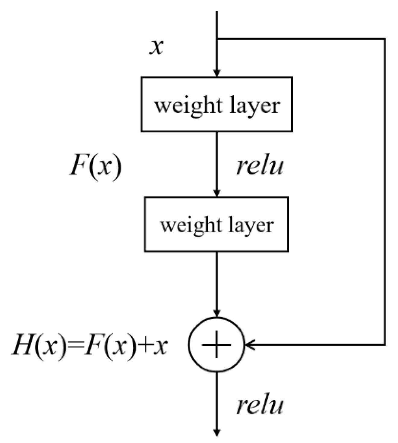
When the CNN model has more convolution layers, there will be more neurons accordingly. Theoretically, the higher the expression degree of the network is, the stronger the fitting ability will be. However, in practical training, gradient explosion and gradient dispersion occur easily with the increase in network layers. He et al. studied the CNN model with residual connection in depth [27]. On the basis of identity mapping theory, the deep residual CNN model assumes that a network with fewer layers has reached the saturation state and then adds the identity mapping layer of the output. The theoretical error is consistent with the previous model, so identity mapping is used to transfer the output of the previous layer to the next layer, which is the design idea of residual CNN. The model adopts the network structure of jump connection to superimpose the shallow and deep features, which can effectively avoid the loss of shallow features during network training. The residual connection structure is shown in Figure 6, in which $x$ is the input of the current unit, and $F(x)$ is the mapping output of the current unit processed by the nonlinear transformation function. In the forward propagation process of CNN, not only is the mapping result of each current unit used as the input of the next unit, but the input of the current unit is also directly connected and added to the input of the next unit to realize the jump connection. Therefore, the input of the next unit is

$$H(x)=F(x)+x.$$

(16)

In comparison with traditional CNN, the most obvious feature of the CNN model with a residual connection is that many branches can connect the input directly to the later layer. The deep residual CNN network builds a residual block model to avoid the gradient disappearance problem caused by excessive convolution and pooling layers of the traditional CNN. The number of layers of the traditional CNN is generally small, and the deep residual CNN model even has hundreds of convolution and pooling layers. The residual CNN model only needs to extract the difference information between the input and output, which reduces the complexity of training objectives and the convergence time required for network model training.

4.2.3. CNN Model Construction

In practical training, with the increase in network layers, gradient explosion and gradient dispersion, as well as other problems, lead to poor backpropagation training effect, that is, the performance of deep network with only increasing the number of layers is poor. Compared with other CNN models, residual CNN avoids the overfitting problem caused by gradient disappearance, which can be used to build a deeper network architecture and maintain the accuracy of the model. Based on the above considerations, the method proposed in this paper used the residual CNN classification model. As a representative model in residual CNN, the ResNet18 model has excellent recognition performance. In this paper, ResNet18 was used as the backbone network, and its framework is shown in Figure 7. First, there exists a convolution layer with dimension of 7 × 7, followed by four ResBlocks. There also exists a pool layer and a fully connected layer at the rear. Because the texture information of the underwater acoustic feature image is fine, the convolution kernel size of the convolution layer is set to 3 × 3 except for the first convolution layer. To fully use the edge information and ensure that the size of convolution layer output is proper, the padding value is set to 1. To adapt to the characteristics of underwater acoustic data, the CNN model adopted in this paper removed the pooling layer in the original ResNet18 model to retain more characteristic information in the input data. In addition, it changed the input layer, the fully connected layer, and the output layer to the size suitable for this research task. The CNN model optimization algorithm was set as the stochastic gradient descent with momentum (SGDM) algorithm, which was because the SGDM can adjust parameters accurately to obtain excellent recognition performance. The number of batch training samples was 128, and the learning rate was 0.0001. In order to avoid overfitting, the batch normalization layer was set after the convolution layer, the L2 normalization (weight decay) coefficient was set to 0.0001, and the dropout layer with a ratio of 0.5 was also set.

5. Analysis and Verification of Experimental Data

5.1. Extraction of Input Features

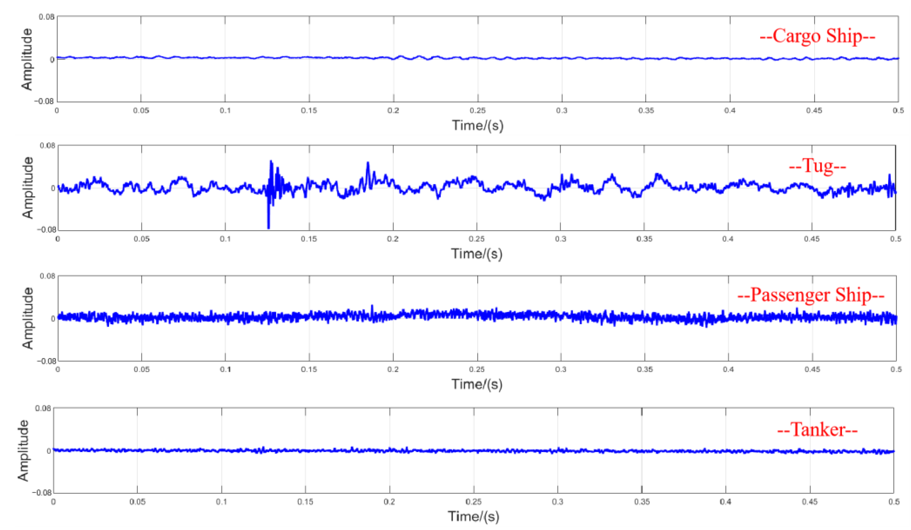
The ship audio data used in this paper were from the DeepShip dataset [28], which includes four types of ships: tug, cargo, tanker, and passenger ship. The data were acquired using a single-channel acquisition system, with a sampling frequency of 32 kHz. If the complete database is used, the number of samples is large enough to support the training of machine learning in theory, and the necessity of using data augmentation is reduced. However, in the actual environment, the acquisition of underwater acoustic samples is often very complex and difficult, and the measured samples are relatively scarce. The research on the effective recognition of underwater acoustic targets with only a small number of samples has more application value, so this paper only used part of the database. The information of the raw recordings of ships used in this paper is shown in

Table 1. The information of raw recordings of ships.

Category	Specific Number, Name, and Recording Time
Tug	9, MILLENNIUMSTAR, 20171115 40, SEASPAN COMMANDER, 20171203 49, SEASPAN EAGLE, 20171210
Cargo	15, NEW NADA, 20171114 38, ARIES LEADER, 20171123 62, ANASTASIA, 20171202
Tanker	10, NAVE ORBIT, 20160602 18, OVERSEAS ATHENS, 20160619 24, HIGH ENDURANCE, 20160710
Passenger	9, CARNIVAL LEGEND, 20160516 16, MALASPINA, 20160604 29, CRYSTAL SERENITY, 20160727

. The audios of three ships were selected for each type of ship. A total of 1,487,488 samples were extracted from each type of ship to obtain the underwater acoustic characteristics. The original signals of various types of ships are shown in Figure 8. The proposed method was developed on a workstation with 11th Gen Intel(R) Core(TM) i7-1165G7 CPU*8. The code was written using MATLAB R2020b (https://www.mathworks.com/ (accessed on 18 October 2020)).

In this paper, three common underwater acoustic characteristics were extracted, which were the MFCC, constant Q transform (CQT), and low-frequency analyzer and recorder (LOFAR) spectrum. Their abilities to represent underwater acoustic targets were analyzed and compared. For the MFCC feature, data were divided into frames with a window length of 256 samples and a step size of 128 samples. In the process of extraction, 20 groups of filters were set, and the first- and second-order difference coefficients were obtained, such that each segment of data could obtain a 1 × 36 feature vector. A total of 11,620 segments of the MFCC feature were extracted from each type of ship’s audio data, with a total of 46,480 segments. For the LOFAR spectrum, it could be obtained by continuous sampling of the signal and short-time Fourier transform (STFT) of continuous signal samples. The frequency interval of the STFT was set to 10 Hz. For the CQT, it used sampling points of frequency domain with exponential distribution [29]. The number of bins per octave was set to 12. Since the frequency of the ship audio was mainly concentrated at low frequency, the signal frequency analysis range of the CQT and LOFAR spectrum was set to 0–2500 Hz. The data framing of the CQT and LOFAR spectrum was consistent with the MFCC feature. For tug, cargo, tanker, and passenger ships, the MFCC, CQT, and LOFAR spectrum of 2.5 s sound data were selected as an example, as shown in Figure 9, Figure 10 and Figure 11, respectively.

The statistical histograms of the MFCC, CQT, and LOFAR spectrum are shown in Figure 12. The different colors represent different types of ships; Figure 12a shows that the different types of ships had obvious differences in terms of the MFCC, which were specifically expressed in the location, shape, skewness, and kurtosis of the distributions. Figure 12b,c show that the audios of different types of ships were very similar in terms of the CQT and LOFAR spectrum, which greatly reduced the recognition performance. Therefore, compared with the CQT and LOFAR spectrum, the characteristic information of the MFCC was more representative.

5.2. Expansion of Samples by Data Augmentation

The feature vectors of every five consecutive frames were spliced in parallel to generate a two-dimensional matrix, which was used to generate the color image as the input feature of a single sample. Taking the MFCC feature as an example, Figure 13 shows the single image sample of each type of ship. A total of 2324 samples were obtained for each type of ship, of which 3/4 image samples were randomly selected for the training of the model, and the remaining 1/4 were used for the testing, such that 1743 training samples and 581 test samples were obtained for each type of ship. Therefore, 6972 labeled samples were included in the training set, and 2324 samples were included in the test set.

The image contrast ranges were set to 0.1–0.9, 0.2–0.8, and 0.3–0.7. The original feature image could obtain three generated images by adjusting the contrast. The tug was taken as an example, as shown in Figure 14. The generation results of the DCGAN model are shown in Figure 15. A single original feature image sample could be trained by the DCGAN model to obtain a generated image sample. The results showed that after substantial training, the generation results were close to the actual original feature image. For an original feature image, this paper used the data augmentation method to obtain four generated feature images. Like the original images, the generated images could also be used as the input feature of the model to expand the training samples, that is, the number of training samples for each type of ship was expanded from 1743 to 8715.

5.3. Recognition Results

In this paper, the recognition performance of SVM, common CNN, VGG19, and ResNet18 was compared. For the SVM, the image sample was transformed into the feature matrix used to input the model. For the common CNN model, the number of layers was relatively small. The model had three convolution layers, which was expressed as 3_CNN. For the VGG19 model, it contained 16 convolution layers, five pooling layers, and three full connection layers [11]. The parameters of the input layers were adjusted to match the input features of this paper. ResNet18 and VGG19 had 17 and 16 convolution layers, respectively, and their depths were similar; the obvious difference between the two models was that the ResNet18 model used residual connection, while the VGG19 model only increased the number of convolution layers on the basis of traditional CNN. The recognition accuracy, precision, and recall were taken as the measurement index of the recognition results, and the formulas are as follows:

$$Accuracy=\frac{TP+TN}{TP+TN+FP+FN},$$

(17)

$$precision=\frac{TP}{TP+FP},$$

(18)

$$recall=\frac{TP}{TP+FN},$$

(19)

$$F1\text{-}score=2*\frac{precision*recall}{precision+recall},$$

(20)

where TP, TN, FP, and FN represent true positive, true negative, false positive, and false negative, respectively.

Table 2. Recognition accuracy (%) for different types of ships’ target signals with the input of the MFCC.

Method	A	B	C	D	Total
SVM	78.55	78.38	79.92	77.85	78.68
SVM_Aug	80.29	81.31	80.96	79.32	80.47
3_CNN	83.18	81.91	82.35	81.03	82.12
3_CNN_Aug	88.95	86.21	87.72	85.52	87.10
VGG19	85.19	87.35	86.03	86.93	86.38
VGG19_Aug	87.24	89.52	89.15	90.39	89.08
ResNet18	93.11	92.24	92.98	91.62	92.48
ResNet18_Aug	96.85	96.23	97.01	95.38	96.37

shows the recognition accuracy for different types of ships’ target signals with the input of the MFCC. Tug, cargo, tanker, and passenger ships are represented as A, B, C, and D, respectively. Each method compares the use of data augmentation technology with the use of no data augmentation technology, and Aug indicates the use of data augmentation technology.

The accuracy comparison of the MFCC, CQT, and LOFAR spectrum by different methods are shown in

Table 3. Accuracy comparison (%) for the MFCC by different methods.

Method	Accuracy	Precision	Recall	F1 Score
SVM	78.68	78.76	78.61	78.68
SVM_Aug	80.47	80.58	80.42	80.50
3_CNN	82.12	82.15	82.10	82.13
3_CNN_Aug	87.10	87.15	87.13	87.14
VGG19	86.38	86.42	86.40	86.41
VGG19_Aug	89.08	89.11	89.07	89.09
ResNet18	92.48	92.49	92.47	92.48
ResNet18_Aug	96.37	96.40	96.39	96.40

,

Table 4. Accuracy comparison (%) for the CQT by different methods.

Method	Accuracy	Precision	Recall	F1 Score
SVM	72.56	72.61	72.52	72.57
SVM_Aug	76.33	76.40	76.32	76.36
3_CNN	79.61	79.68	79.59	79.64
3_CNN_Aug	83.89	83.95	83.80	83.87
VGG19	81.08	81.19	81.05	81.12
VGG19_Aug	85.23	85.24	85.17	85.21
ResNet18	87.35	87.36	87.32	87.34
ResNet18_Aug	91.92	91.96	91.90	91.93

and

Table 5. Accuracy comparison (%) for the LOFAR spectrum by different methods.

Method	Accuracy	Precision	Recall	F1 Score
SVM	68.12	68.18	68.10	68.14
SVM_Aug	71.41	71.43	71.37	71.40
3_CNN	75.03	75.05	74.98	75.02
3_CNN_Aug	77.45	77.46	77.42	77.44
VGG19	78.01	78.07	77.99	78.03
VGG19_Aug	81.52	81.55	81.48	81.52
ResNet18	86.29	86.33	86.27	86.30
ResNet18_Aug	88.49	88.52	88.48	88.50

, respectively. Image samples generated by different features were input into the models. The MFCC features were obtained according to the human ear auditory mechanism, which can extract the feature information of the low-frequency part more effectively, and the frequency of the ship audios was mainly concentrated in the low-frequency part. Although the CQT could also contain a large amount of detailed information in the low-frequency part of the signal, it was more suitable for the scenes with long data frames. In the underwater acoustic environment, the samples were relatively scarce. The data frames adopted in this paper were of more application value. The LOFAR spectrum lacked the feature information of the low-frequency part, and it only performed a relatively preliminary processing on the original sound signal, while other features obtained the feature information close to the recognition task. Therefore, for the machine learning model, it was more difficult to recognize with the input of the LOFAR spectrum. The results showed that the recognition accuracy of the MFCC feature was better than that of other features at the same method. The accuracy, precision, recall, and F1 score of the ResNet18_Aug model with the input of the MFCC were 96.37%, 96.40%, 96.39%, and 96.40%, respectively. Therefore, the method proposed in this paper selected the MFCC as the input feature.

Figure 16 shows a comparison of recognition accuracy by different classification methods with the input of the MFCC using data augmentation technology and not using data augmentation technology. The results showed that for the same method, the recognition performance could be significantly improved by using data augmentation technology. In comparison with the traditional machine learning model, CNN had the advantages of local perception and weight sharing, so the recognition results of SVM were the worst. Since increasing the depth of the network could improve the recognition performance of CNN to a certain extent, the recognition results of VGG19 were better than those of 3_CNN. The deeper CNN model with residual connection could extract more abundant data features and avoid the overfitting problem caused by gradient disappearance. Therefore, the recognition performance of ResNet18 was better than that of VGG19. The ResNet18_Aug model had the best recognition results, which was due to the ResNet18_Aug model combining the data expansion advantages of data augmentation technology and the ability of residual CNN to extract deep features.

In order to more fully analyze the recognition performance of different methods, the confusion matrix of recognition results with the input of the MFCC by different methods is shown in Figure 17. The results showed that SVM, SVM_Aug, and 3_CNN had a large number of misjudged test samples, that is, these methods could not achieve effective recognition. In the case of the requirement without high accuracy, VGG19_Aug and ResNet18 could realize effective recognition. At the same method, using data augmentation technology, the number of misjudged test samples was significantly reduced. The recognition results of ResNet18_Aug were better than those of other models, and only a few test samples were misjudged, which showed that the comprehensive application of deep residual CNN and data augmentation technology would greatly improve the recognition performance.

6. Conclusions

As the depth and complexity of machine learning models increase, traditional methods have gradually failed to meet the requirements of intelligent development in the field of underwater acoustic recognition. In recent years, machine learning methods have been widely used in underwater target recognition. However, the sample data of underwater acoustic targets are relatively scarce, which limits the application of machine learning in actual underwater acoustic recognition. This paper presented a method of underwater acoustic target recognition based on the data augmentation technique and the residual CNN model. The whole process mainly included MFCC feature extraction, data augmentation processing, and ResNet18 model recognition. On the basis of traditional data augmentation techniques such as adjusting image contrast, this paper used the DCGAN model to expand underwater acoustic data and compared the SVM, 3_CNN, VGG19, and ResNet18 models. The results showed that the recognition accuracy of the MFCC feature was better than that of the CQT and LOFAR spectrum for the same method, and using data augmentation method could obviously improve the recognition performance; ResNet18_Aug was superior to other models and achieved 96.37% recognition accuracy. In addition, although this method was used for ship target recognition in this paper, it is not limited to this. In the field of passive acoustics, this method is also applicable to other target voice recognition, such as natural sound and underwater vocal biometrics. However, the method proposed in this paper only verified the recognition of single underwater acoustic targets. The subsequent research can be extended to multiple targets and explore the effective recognition in cases with fewer measured samples.

References

1. Kamal, S.; Mohammed, S.K.; Pillai, P.R.S.; Supriya, M.H. Deep learning architectures for underwater target recognition. In Proceedings of the 2013 Ocean Electronics (SYMPOL), Kochi, India, 23–25 October 2013; pp. 48–54. [Google Scholar]
2. Shamir, L.; Yerby, C.; Simpson, R.; von Benda-Beckmann, A.M.; Tyack, P.; Samarra, F.; Miller, P.; Wallin, J. Classification of large acoustic datasets using machine learning and crowdsourcing: Application to whale calls. J. Acoust. Soc. Am. 2014, 135, 953–962. [Google Scholar] [CrossRef] [PubMed] [Green Version]
3. Yue, H.; Zhang, L.; Wang, D.; Wang, Y.; Lu, Z. The Classification of Underwater Acoustic Targets Based on Deep Learning Methods. In Proceedings of the 2017 2nd International Conference on Control, Automation and Artificial Intelligence, Sanya, China, 25–26 June 2017. [Google Scholar]
4. Shiu, Y.; Palmer, K.J.; Roch, M.A.; Fleishman, E.; Liu, X.; Nosal, E.M.; Helble, T.; Cholewiak, D.; Gillespie, D.; Klinck, H. Deep neural networks for automated detection of marine mammal species. Sci. Rep. 2020, 10, 607. [Google Scholar] [CrossRef] [PubMed] [Green Version]
5. Mishachandar, B.; Vairamuthu, S. Diverse ocean noise classification using deep learning. Appl. Acoust. 2021, 181, 108141. [Google Scholar] [CrossRef]
6. Song, G.; Guo, X.; Wang, W.; Ren, Q.; Li, J.; Ma, L. A machine learning-based underwater noise classification method. Appl. Acoust. 2021, 184, 108333. [Google Scholar] [CrossRef]
7. Yang, H.; Li, J.; Sheng, M. Underwater acoustic target multi-attribute correlation perception method based on deep learning. Appl. Acoust. 2022, 190, 108644. [Google Scholar]
8. Escobar-Amado, C.D.; Badiey, M.; Pecknold, S. Automatic detection and classification of bearded seal vocalizations in the northeastern Chukchi Sea using convolutional neural networks. J. Acoust. Soc. Am. 2022, 151, 299–309. [Google Scholar] [CrossRef]
9. Luo, W.; Yang, W.; Zhang, Y. Convolutional neural network for detecting odontocete echolocation clicks. J. Acoust. Soc. Am. 2019, 145, EL7–EL12. [Google Scholar] [CrossRef] [Green Version]
10. Krizhevsky, A.; Sutskever, I.; Hinton, G. ImageNet Classification with Deep Convolutional Neural Networks. Adv. Neural Inf. Process. Syst. 2012, 25, 1097–1105. [Google Scholar] [CrossRef] [Green Version]
11. Simonyan, K.; Zisserman, A. Very Deep Convolutional Networks for Large-Scale Image Recognition. arXiv 2014, arXiv:1409.1556. [Google Scholar]
12. Zeiler, M.; Fergus, R. Visualizing and understanding convolutional networks. In Proceedings of the Computer Vision–ECCV 2014: 13th European Conference, Zurich, Switzerland, 6–12 September 2014; pp. 818–833. [Google Scholar]
13. Szegedy, C.; Liu, W.; Jia, Y.; Sermanet, P.; Reed, S.; Anguelov, D.; Erhan, D.; Vanhoucke, V.; Rabinovich, A. Going Deeper with Convolutions. In Proceedings of the IEEE Conference on Computer Vision and Pattern Recognition, Columbus, OH, USA, 23–28 June 2014. [Google Scholar]
14. Szegedy, C.; Ioffe, S.; Vanhoucke, V.; Alemi, A. Inception-v4, inception-resnet and the impact of residual connections on learning. arXiv 2016, arXiv:1602.07261. [Google Scholar] [CrossRef]
15. Jie, H.; Li, S.; Gang, S.; Albanie, S. Squeeze-and-Excitation Networks. IEEE Trans. Pattern Anal. Mach. Intell. 2020, 42, 2011–2023. [Google Scholar]
16. Fong, R.; Vedaldi, A. Occlusions for effective data augmentation in image classification. In Proceedings of the 2019 IEEE/CVF International Conference on Computer Vision Workshop (ICCVW), Seoul, Republic of Korea, 27–28 October 2019. [Google Scholar]
17. Baek, F.; Park, S.; Kim, H. Data augmentation using adversarial training for construction-equipment classification. arXiv 2019, arXiv:1911.11916. [Google Scholar]
18. Goodfellow, I.; Pouget-Abadie, J.; Mirza, M.; Xu, B.; Warde-Farley, D.; Ozair, S.; Courville, A.; Bengio, Y. Generative Adversarial Nets, Neural Information Processing Systems; MIT Press: Cambridge, MA, USA, 2014. [Google Scholar]
19. Yang, J.; Kannan, A.; Batra, D.; Parikh, D. LR-GAN: Layered Recursive Generative Adversarial Networks for Image Generation. arXiv 2017, arXiv:1703.01560. [Google Scholar]
20. Radford, A.; Metz, L.; Chintala, S. Unsupervised representation learning with deep convolutional generative adversarial networks. arXiv 2015, arXiv:1511.06434. [Google Scholar]
21. Mirza, M.; Osindero, S. Conditional Generative Adversarial Nets. arXiv 2014, arXiv:1411.1784. [Google Scholar]
22. Yang, K.; Zhou, X. Deep learning classification for improved bicoherence feature based on cyclic modulation and cross-correlation. J. Acoust. Soc. Am. 2019, 146, 2201–2211. [Google Scholar] [CrossRef] [PubMed]
23. Gulrajani, I.; Ahmed, F.; Arjovsky, M.; Dumoulin, V.; Courville, A. Improved training of wasserstein GANs. arXiv 2017, arXiv:1704.00028. [Google Scholar]
24. Drucker, H.; Burges, C.J.C.; Kaufman, L.; Smola, A.; Vapnik, V. Support vector regression machines. In Advances in Neural Information Processing Systems; Mozer, M.C., Jordan, M., Petsche, T., Eds.; MIT Press: Cambridge, MA, USA, 1997; Volume 9, pp. 155–161. [Google Scholar]
25. Smola, A.J.; Schölkopf, B. A tutorial on support vector regression. Stat. Comput. 2004, 14, 199–222. [Google Scholar] [CrossRef] [Green Version]
26. Fukushima, K.; Miyake, S.; Ito, T. Neocognitron: A neural network model for a mechanism of visual pattern recognition. IEEE Trans. Syst. Man Cybern. 1983, SMC-13, 826–834. [Google Scholar] [CrossRef]
27. He, K.; Zhang, X.; Ren, S.; Sun, J. Deep residual learning for image recognition. In Proceedings of the IEEE Conference on Computer Vision and Pattern Recognition, Las Vegas, NV, USA, 27–30 June 2016; pp. 770–778. [Google Scholar]
28. Irfan, M.; Jiangbin, Z.; Ali, S.; Iqbal, M.; Masood, Z.; Hamid, U. DeepShip: An Underwater Acoustic Benchmark Dataset and a Separable Convolution Based Autoencoder for Classification. Expert Syst. Appl. 2021, 183, 115270. [Google Scholar] [CrossRef]
29. Brown, J.C. Calculation of a constant Q spectral transform. J. Acoust. Soc. Am. 1998, 89, 425–434. [Google Scholar] [CrossRef] [Green Version]
Figure 1. Overall flow diagram.
Electronics 12 01206 g001
Figure 2. MFCC feature extraction flowchart.
Electronics 12 01206 g002
Figure 3. Frame diagram of the discriminator.
Electronics 12 01206 g003
Figure 4. Frame diagram of the generator.
Electronics 12 01206 g004
Figure 5. Typical CNN model.
Electronics 12 01206 g005
Figure 6. Residual connection structure.
Electronics 12 01206 g006
Figure 7. ResNet18 model framework.
Electronics 12 01206 g007
Figure 8. Waveform of ship’s original signal in DeepShip dataset.
Electronics 12 01206 g008
Figure 9. MFCC features of different types of ships.
Electronics 12 01206 g009
Figure 10. CQT of different types of ships.
Electronics 12 01206 g010
Figure 11. LOFAR spectrum of different types of ships.
Electronics 12 01206 g011
Figure 12. Statistical histograms of the MFCC, CQT, and LOFAR spectrum.
Electronics 12 01206 g012
Figure 13. The single image sample of each type of ship.
Electronics 12 01206 g013
Figure 14. Tug image samples at different contrast ranges.
Electronics 12 01206 g014
Figure 15. DCGAN model generation samples of different types of ships.
Electronics 12 01206 g015
Figure 16. Comparison of recognition accuracy with the input of the MFCC using data augmentation technology and not using data augmentation technology.
Electronics 12 01206 g016
Figure 17. Confusion matrix of recognition results with the input of the MFCC by different methods.
Electronics 12 01206 g017