Article

Modeling to Correct the Effect of Soil Moisture for Predicting Soil Total Nitrogen by Near-Infrared Spectroscopy

College of Mechanical and Electrical Engineering, Hainan University, Haikou 570228, China
*
Author to whom correspondence should be addressed.
Electronics 2023, 12(6), 1271; https://doi.org/10.3390/electronics12061271
Submission received: 13 February 2023 / Revised: 2 March 2023 / Accepted: 2 March 2023 / Published: 7 March 2023
(This article belongs to the Section Artificial Intelligence)

Abstract

:
Near-infrared (NIR) spectroscopy can improve the efficiency of soil property prediction, such as that of soil total nitrogen (TN) content. However, soil spectra are very sensitive to soil moisture content, which is a crucial factor affecting the accuracy of soil nutrient composition prediction. In response to this issue, the goal of this study is to identify the best model to correct the effect of soil moisture for predicting soil total nitrogen by near-infrared spectroscopy. The 107 collected soil samples were divided into six different water content (0%, 5%, 10%, 15%, 20%, and 25%) sample groups. Then, five correction methods, including direct standardization (DS), piecewise direct standardization (PDS), external parameter orthogonalization (EPO), spectral space transformation (SST), and slope/bias (S/B), were executed. Finally, partial least squares regression (PLSR) models were established to forecast TN content. The results showed that SST could minimize the influence of moisture. Furthermore, SST–PLSR had the best TN content prediction accuracy: R p 2 (the coefficient of determination of the prediction set) in the range of 0.81–0.82, RMSEP (the root mean square error of the prediction set) in the range of 0.09–0.10 g/kg, and RPD (ratio of performance to deviation) in the range of 2.32–2.40. Therefore, the dry soil prediction model is competent for wet soil samples and could achieve preciseness in TN content prediction. The use of SST can effectively eliminate the influence of moisture and achieve high-precision TN prediction in wet soil samples. Additionally, the introduction of SST expands the application scope of soil nutrient prediction models and increases model robustness.

1. Introduction

Soil total nitrogen (TN) is an integral part of soil nutrients and can reflect soil fertility. Adequate nitrogen is essential for the growth of rubber trees [1], and TN content is positively correlated with rubber yield [2,3,4]. However, the longer the rubber tree remains planted in the soil, the more severe the total nitrogen loss in the soil is. For the healthy growth of rubber trees and the supply of natural rubber, it is necessary to detect the total nitrogen content of the soil quickly.
The traditional determination method of soil TN content is the chemical analysis method, divided into the Kjeldahl and Dumas combustion methods [5]. There are several problems with the traditional chemical analysis method, such as high consumption of chemical reagents, lengthy analysis time, and cumbersome operation [6]. In the last few years, many researchers have found that near-infrared (NIR) spectroscopy can effectively improve the prediction efficiency of soil TN [7,8,9]. However, several factors affect the soil spectral characteristics, such as water, temperature, and particle size [8,10]. Since –OH groups of soil moisture can significantly affect the near-infrared spectral reflectance, soil moisture is considered one of the key elements reducing the accuracy of soil nutrient composition measurements [11,12]. Therefore, soil samples need to be dried to predict soil nutrients using NIR. However, the drying, grinding, and sieving of soil samples is a labor-intensive and time-consuming process [13]. Although portable spectrometers can save costs by collecting soil spectra directly in the field, soil moisture can still reduce the accuracy of predicting soil nutrient content. Therefore, research to remove the effect of moisture is crucial to improve the accuracy of portable spectrometer measurements and the robustness of prediction models.
To eliminate the negative effects of moisture, researchers have tried several different approaches: external parameter orthogonalization (EPO) [6,14], direct standardization (DS) [15], piecewise direct standardization (PDS) [14], orthogonal signal correction (OSC) [14,16], slope/bias (S/B) correction method [15], etc. Although the above methods can improve the effect of wet soil spectral models, the accuracy of these methods is still not as good as that of dry soil spectral models. As soil moisture increases, elimination of the influence of moisture in models becomes less effective. On the other hand, climate, parent material, vegetation type, soil texture, and land use affect TN, and show different states [17]. Thus, the soil spectral curve has different characteristics, such as sharp peaks or smoothness. From this perspective, the spectral correction methods for different soils are different [18]. The EPO method is considered the most effective way to mitigate the impacts of soil moisture [19]. However, the accuracy of wet soil prediction models after EPO correction is still far from the accuracy of dry soil prediction models, which may be due to the fact that EPO is not suitable for smoother spectra. In addition, EPO assumes that the original spectral matrix of wet soil consists of three parts: the useful part related to soil properties, the part affected by moisture, and the independent residual part, but researchers ignore the influence of the independent residual part in practical applications [6], resulting in the improvement effect not being maximized. Therefore, new methods need to be investigated to mitigate the effects of moisture.
Spectral space transformation (SST) was first applied to solve the incompatibility of calibration models between master and slave instruments. SST has no requirements for the type of spectra, regardless of whether the spectra is smooth, sharp, or discontinuous [20,21]. It has been used on plants and achieved good results [21]. However, no researchers have investigated the potential of SST in eliminating the environmental noise effects of spectral curves. The rubber forest soil in Hainan Province is mainly brick-red soil [22], and the spectral curve of brick-red soil is relatively smooth. Therefore, this paper intends to use brick-red soil samples to explore the effect of SST on the removal of soil moisture effects in soil spectra.
Based on the above analysis, in order to eliminate the influence of moisture, improve the accuracy of soil total nitrogen prediction, and improve the robustness of the spectral prediction model, this paper uses 107 brick-red soil samples collected from the rubber forest farm in Danzhou City, Hainan Province, China. It is proposed to use SST to correct the wet soil spectra to eliminate the influence of moisture on the soil total nitrogen spectra prediction model, and compare it with DS, PDS, EPO, and S/B to verify whether SST can minimize the influence of soil moisture on the prediction results. Furthermore, it further provides ideas for reducing prediction errors caused by factors such as soil structure conditions.

2. Materials and Methods

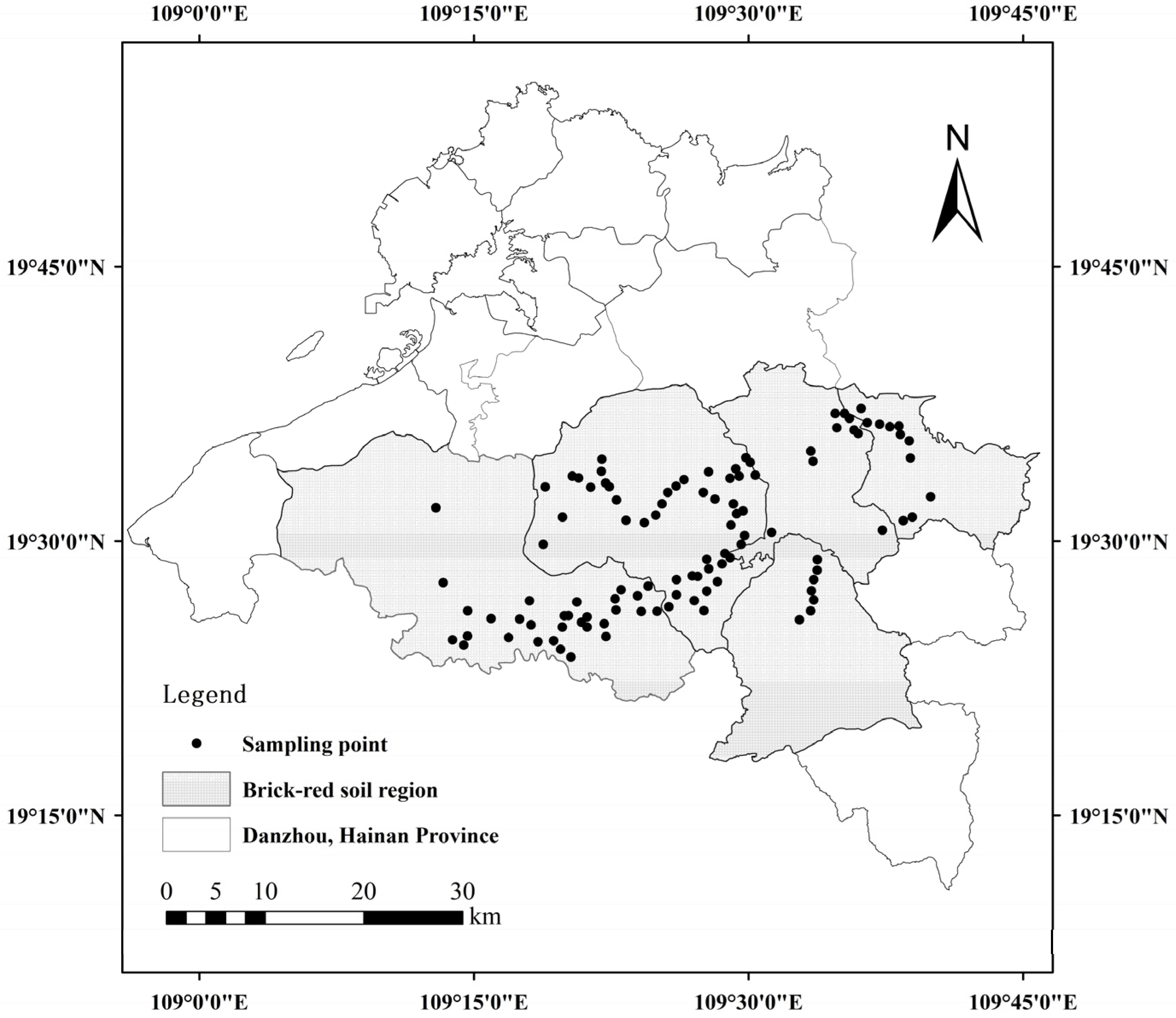
2.1. Study Area and Soil Collection

A total of 107 soil samples were collected from 13 rubber forest farms (19°40′–19°65′ N, 109°20′–109°70′ E) in Danzhou City, Hainan Province, China (Figure 1), in the summer of 2021. Danzhou city is located on the southern edge of the East Asian continental monsoon climate. The tropical monsoon climate is hot and humid. It is very suitable for planting rubber trees. When choosing soil plots, we chose to avoid potholes and overgrown areas. According to the soil classification standard of the World Reference Base for Soil Resources (WRB), the rubber forest soil in Danzhou City belongs to the brick-red loam class of iron bauxite and is a weakly acidic latex soil, and its parent materials are mainly sand shale and granite. The size of the sample plots was 10 × 10 m, and the straight-line distance between each plot was at least 1 km. The five-point sampling method was used to collect topsoil at a 0–20 cm depth in each plot. After thorough mixing, a soil sample was formed, and the number and location information of the sample were recorded accordingly.
During sample preparation, a portion of each soil sample was selected and sent to the laboratory to determine the TN content by the Kjeldahl method [23] and the remainder of the sample was dried in a drying oven at 110 °C for 4 h. The dried sample was sieved to remove the gravel with a 1 mm stainless steel sieve. Finally, the sieved soil was placed in a transparent Petri dish to collect the spectral data.

2.2. Acquisition of Soil Spectra

Soil spectra were collected using a hyperspectral imager (GaiaField-F-N17, ZOLIX INSTRUMENTS Co., Ltd., Beijing, China). The darkroom of the spectrometer consists of four halogen lamps and one specimen stage. The halogen lamps are about 0.8 m away from the stage, and their inclination angle is about 45°. Samples were placed on a moving stage that scans at a uniform speed. A whiteboard was used for black and white correction before data collection. The spectral resolution of this hyperspectrometer is 4 nm with a sampling interval of 3.3 nm.
The dried soil samples were placed on the mobile platform, and the hyperspectrometer collected their hyperspectral data within the wavelength range 866–1701 nm. After the black and white correction process, 80 × 80 pixel interceptions of the hyperspectral data were averaged to obtain the average spectra. Considering that the wavelengths at both ends had serious noise, the spectral bands in ranges 866–966 nm and 1692–1701 nm were removed, and 222 spectral bands were retained. In this paper, the sample set partitioning based on the joint x–y distance (SPXY) algorithm divided all 107 soil samples into 86 calibration sets and 21 prediction sets according to the ratio of 4:1 (SPXY algorithm uses TN content values as the y variable and soil spectrum as the x variable, and uses these two variables to calculate the distance between samples to achieve division of the sample set, which can increase the difference and representativeness between samples and improve the stability of the model).
Table 1 shows the descriptive statistical characteristics of TN content (The data in Table 1 were obtained by the Kjeldahl method). The TN content of the entire sample set ranged from 0.13 to 1.74 g/kg, with an average of 0.58 g/kg, a median of 0.53 g/kg, and a standard deviation of 0.25. The statistical characteristics of the calibration set are consistent with the total sample set. The TN content range of the prediction set is smaller than that of the calibration set, indicating that the model is effective within the research range for the prediction set [24].

2.3. Wet Soil Sample Preparation

After spectral collection of all dry soil samples, a specific amount of deionized water was added to each dry soil sample according to Equation (1) to bring the moisture content to 5%. Then, the samples were scanned with a hyperspectral imager after thorough mixing. Finally, the average spectra of samples were calculated. The above experimental steps were repeated to obtain six groups of spectral data of soil samples with moisture contents of 0% (dry soil samples), 5%, 10%, 15%, 20%, and 25%.
y = x wet x dry x dry × 100 %
In Equation (1), y represents water content, x wet is soil weight after adding water, and x dry is dried soil weight.

2.4. Methods to Remove Moisture Effects

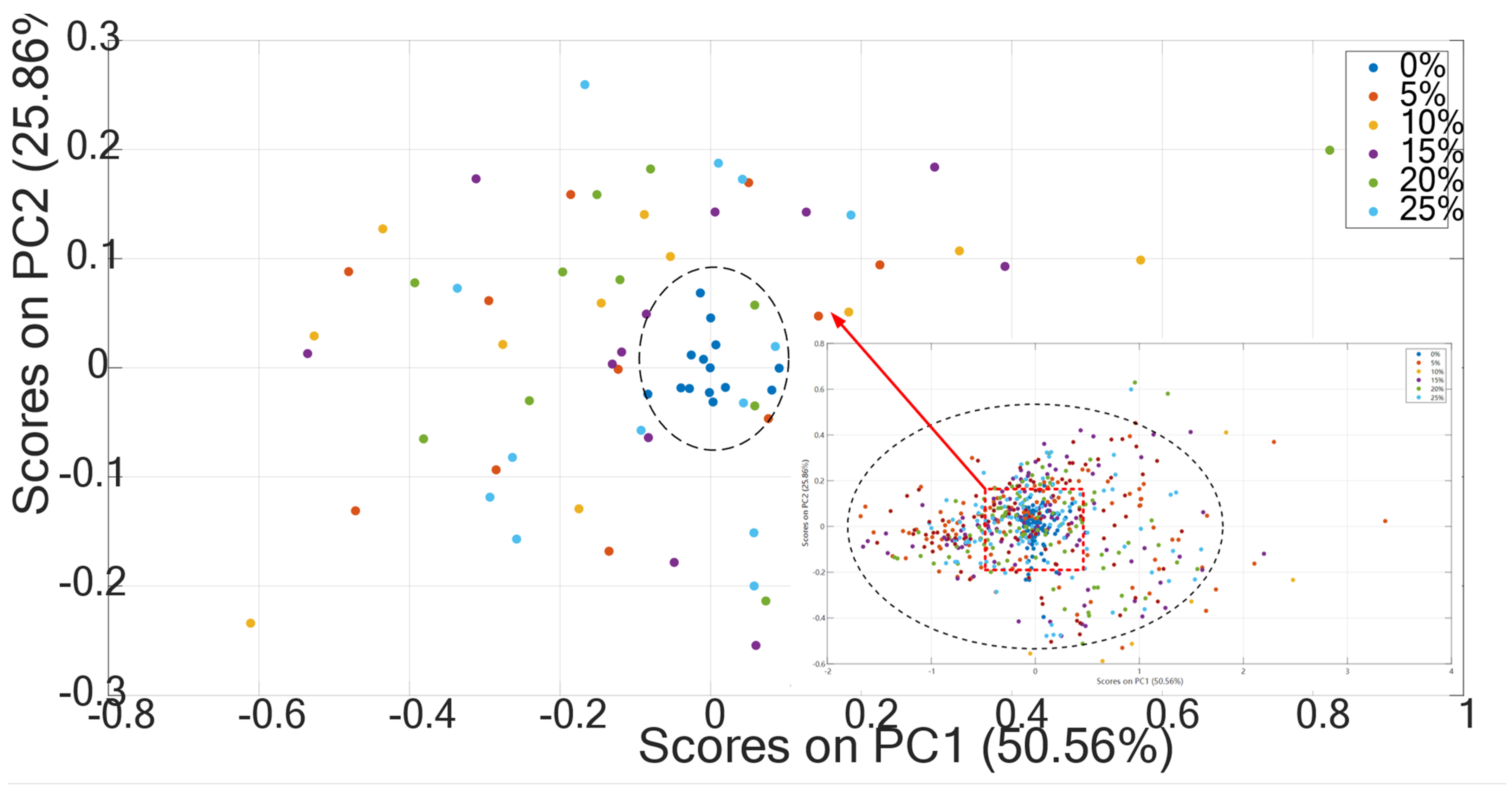
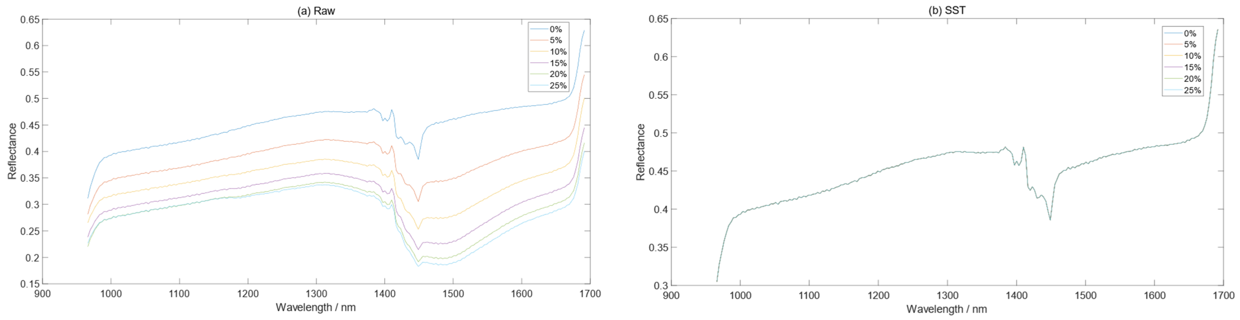
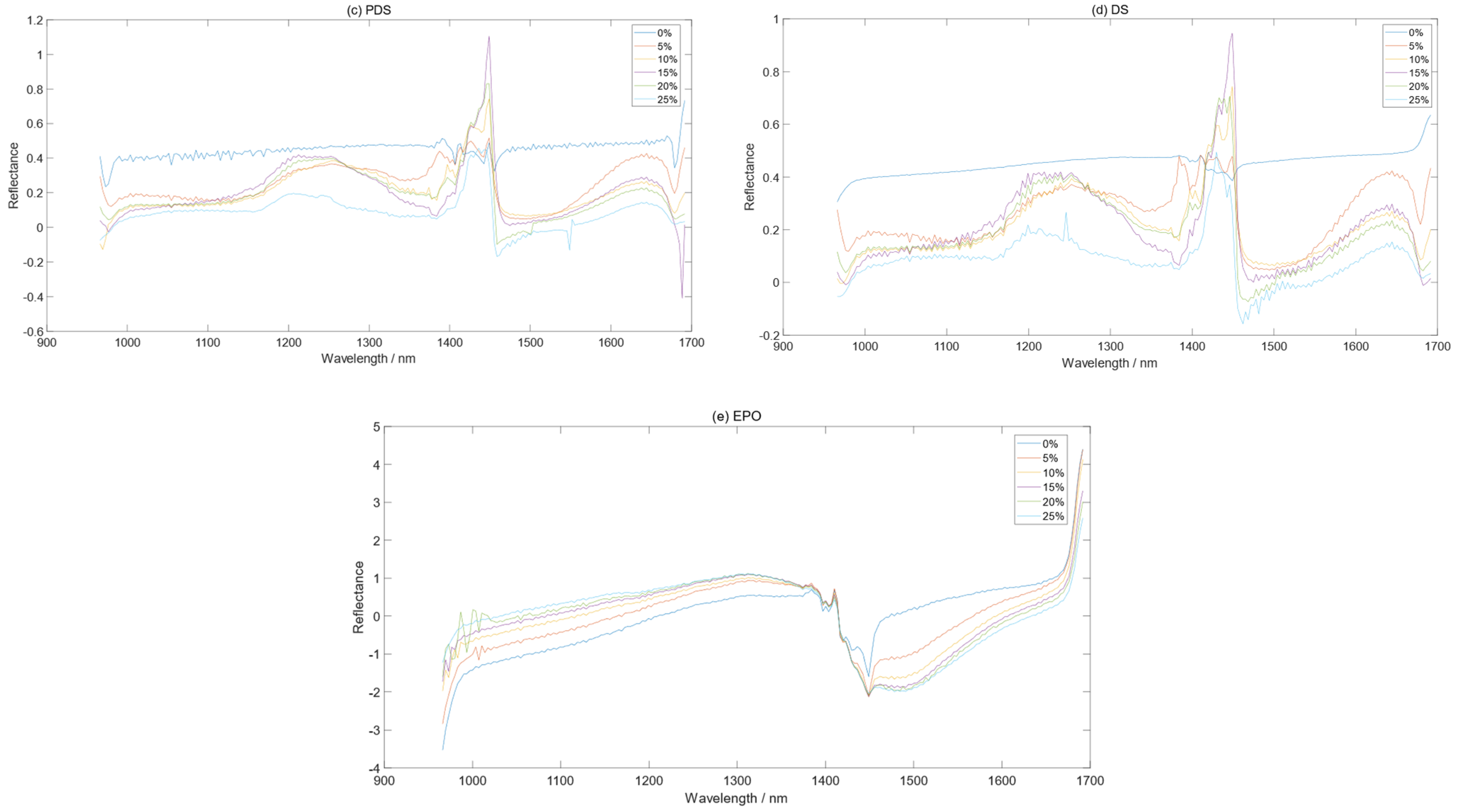
2.4.1. Spectral Space Transformation

Spectral space transformation (SST) is often used to solve the problem of poor model generality due to different times, environments, or machining errors between instruments [20,25]. In this paper, it is assumed that the spectral matrices x dry and x wet are the corresponding spectra of dry soils and wet soils, respectively. Let the joint matrix of x dry and x wet be x c o m b = [ x dry ,   x wet ] ; the singular value decomposition (SVD) of x c o m b is expressed as:
x c o m b = [ U m , U n ] [ Σ m 0 0 Σ n ] [ V m , V n ] T = T m P m T + E = T m [ P d T , P w T ] + E
In Equation (2), T m = U m Σ m ; P m = V m ; E = U n Σ n V n T . The superscript “T” denotes transpose, and the subscripts “m” and “n” denote the corresponding components of spectral information and noise (noise refers to the effect of moisture), respectively. The column number r of P m represents the actual number of spectrally active chemical constituents. The submatrices of P m T = [ P d T , P w T ] , P d T and P w T , have the same number of columns as x dry and x wet , respectively. P d and P w are the loads of x dry and x wet , respectively. E is the residual matrix. When correcting the wet soil spectra with dry soil, the corrected spectra are calculated according to the following equation:
x t = x s ( P w T ) + P d T + x s x s ( P w T ) + P w T
In Equation (3), x s is the spectral matrix of the wet soil test samples, and x t is the spectral matrix of the corrected test samples. The superscript “+” indicates the Moore–Penrose generalized inverse. The transformation matrix F can be separated from Equation (3), as shown in Equation (4):
F = I + ( P w T ) + ( P d T P w T )
In Equation (4), I represent the identity matrix.
As can be seen from the above reasoning process, SST attempts to eliminate spectral differences caused by moisture by transforming between the two spectral spaces spanned by the corresponding spectra of a subset of soil samples under moisture-free and moisture-containing conditions.

2.4.2. Direct Standardization

Direct standardization (DS) is a standard algorithm used for spectral model transformation to eliminate differences caused by different test equipment [15,26]. In this paper, it is used to perform a global linear transformation on the spectra of dry soils and wet soils, and obtain the F transformation matrix, to mitigate the influence of moisture. DS predicts the reflectance of dry soil at each j t h wavelength ( x j ) based on the full spectra of wet soil, and each j t h wavelength is regressed to generate a vector of regression coefficients in the j t h column of the F matrix. Specifically, DS takes the mean values of the dry soil spectral matrix X d and the wet soil spectral matrix X w and then centers them to obtain X d ¯ and X w ¯ . The matrix conversion equation is as follows:
X d ¯ = X w ¯ F
F = X w ¯ 1 X d ¯
In Equation (5), X d ¯ and X w ¯ are both m × n matrices, where m is the number of samples, n is the number of wavelengths, and the size of the F matrix is n × n. In Equation (6), X w ¯ 1 represents the inverse of X w ¯ . When solving the inverse, SVD needs to be used to decompose X w ¯ into three matrices U, S, and V (Equation (7)), then the inverse of X w ¯ can be obtained as shown in Equation (8).
X w ¯ = USV T
X w ¯ 1 = VS 1 U T
Substitute Equation (8) into (6) to obtain the F matrix. In this paper, when calculating the F matrix with the dry and wet soil spectra, the number of samples required by DS was set to 21, and the wet soil spectra can be corrected by applying the transformation matrix F to other wet soil samples.

2.4.3. Piecewise Direct Standardization

Piecewise direct standardization (PDS) achieves spectral normalization by correlating adjacent wavelengths within the window size in the wet soil spectra with the corresponding wavelengths in the dry soil spectra to correct the effects of moisture noise [14]. First, take a window (ik, i + k) near the i t h wavelength of wet soil spectra, and let Y i (Equation (9)) represent the spectral matrix of the wet soil spectra from ik to i + k with a total of 2k + 1 wavelengths. Then, the relationship between Y i and the dry soil spectra Z m , i of the i t h wavelength of the dry soil spectra is obtained:
Y i = [ Z s , i k , Z s , i k + 1 , , Z s , i + k ]
Z m , i = Y i b i
In Equation (10), b i is the regression coefficient vector of the i t h wavelength. Putting all the regression coefficients b i on the main diagonal of the transformation matrix F and setting the other elements to 0, we obtain a diagonal matrix F:
F = diag ( b 1 T , b 2 T , , b i T , , b p T )
In Equation (11), p is the number of wavelengths. The transformation matrix F can convert the wet soil spectra X w into a matrix matching the dry soil spectra X d . The number of samples required for PDS is set to 21, and the wavelength window size is 5.

2.4.4. External Parameter Orthogonalization

External parameter orthogonalization (EPO) is to project wet soil spectra to the space orthogonal to the soil moisture influence factors to be removed to effectively remove the influence of moisture [6,14,19]. The EPO algorithm assumes that the wet soil spectral matrix X consists of three parts: the useful part X u related to TN content, the part X q affected by moisture, and the independent residual matrix R.
X = X u + X q + R
Specifically, the algorithm of EPO is described as follows (the superscript “T” means transpose) [19]:
(1)
Calculate the spectral difference matrix D between the wet soil spectra and the dry soil spectra;
(2)
Perform SVD on the spectral difference combination D T D to obtain the matrix V;
(3)
Define the dimension as 4 and compute the subset V s of V, and   Q = V s V s T ;
(4)
Calculate the projection matrix P, P = I − Q; I represents the identity matrix;
After removing the influence of moisture in X, the corrected spectra are X * = X P ; X * is the useful part X u related to the TN content.

2.4.5. Slope/Bias

The slope/bias (S/B) method uses an algorithm for correction based on prediction results [15]. In this paper, a prediction model G for predicting the TN content of dry soils is first established. Then, the spectral matrix of wet soil samples is randomly selected as X 1 , and the model G is used to directly predict X 1 to obtain the predicted value U 1 of the TN content. It is assumed that the relationship between the actual value U 0 and U 1 is as follows:
U 0 = S l o p e × U 1 + B i a s
The solutions of Slope and Bias use a univariate linear regression equation for fitting, and the principle of the smallest residual sum of squares is followed in the solution process:
S l o p e =   ( U 0 , i U 0 ¯ ) ( U 1 , i U 1 )   ( U 1 , i U 1 ¯ ) 2
B i a s = U 0 ¯ S l o p e × U 1 ¯
After obtaining solutions of Slope and Bias, the model G is used to predict the remaining wet soil spectral matrix X 2 to obtain the predicted value U 2 of the TN content, and then Equation (16) is used to obtain the corrected predicted value U 3 of the soil TN content:
U 3 = S l o p e × U 2 + B i a s

2.5. Model Establishment and Evaluation

The partial least squares regression (PLSR) model has been widely used in soil spectral prediction [6,8,11,12,15,16]. PLSR is a regression algorithm composed of principal component analysis, canonical correlation analysis, and multiple linear regression, which can find the relationship between the spectral matrix X and the soil TN content Y. PLSR considers extracting the principal components in Y and X and maximizing the correlation between them [6].
This study used PLSR to build the model. Three parameters were used to evaluate the performance of the model, including the root mean square error (RMSE), coefficient of determination ( R 2 ), and the ratio of performance to deviation (RPD). R c 2 and R p 2 denote the coefficients of determination of the calibration set and the prediction set, respectively, and RMSEC and RMSEP denote the root mean square errors of the calibration set and the prediction set, respectively. In general, when RPD > 2.0, the closer R 2 is to 1, and the lower the RMSE is, the more substantial the predictive ability of the model is [27,28].

2.6. Flowchart

The flowchart in Figure 2 describes the steps taken in the model’s calibration and validation process for the dry and wet soil spectral data obtained in this study. First, the same preprocessing was performed on dry and wet soil spectral datasets. The result of the prediction model established with the preprocessed dry soil spectra was called the uncorrected TN prediction. Wet soil spectra were corrected using five methods, namely SST, EPO, PDS, DS, and S/B. The result of building the model was called the corrected TN prediction. The performance of the corrected model was evaluated by comparing the corrected model results with the uncorrected model.

3. Results

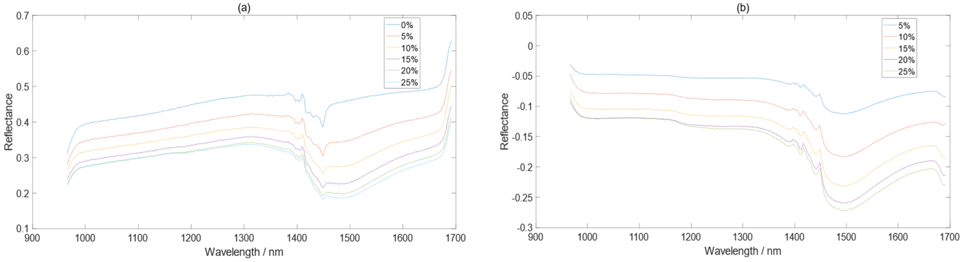
3.1. The Effect of Moisture on the Soil Spectra

The morphological characteristics of the average spectral reflectance curves of soil samples with different water contents are different. In the spectra of dry soil samples (0% moisture content), the most significant absorption band is located around 1450 nm. As the moisture content increased, the soil’s spectral reflectance showed an apparent decreasing trend (Figure 3a). When moisture content is less than 20%, the noise due to moisture in the soil spectra is more pronounced. When the moisture content is ≥20%, the influence of moisture no longer increases evidently. In comparison, the rate of decrease in spectral reflectance tends to be gentle. In particular, the spectra in the range of 966–1450 nm tend to overlap. When the water in the soil pores is saturated, the entire spectral reflectance tends to be stable. With the increase in water content, the depth of the spectral reflection valley between 1400–1500 nm deepens. The difference between the spectral reflectance of wet soil samples with different water contents and the spectral reflectance of dry soil samples (Figure 3b) varies most significantly in the range of 1400–1500 nm, and this change is uneven.
Principal component analysis (PCA) processing was performed on the original soil spectra under different water content conditions. It was found that the distribution of the soil’s spectral PCA scores under different water content conditions were also different. As shown in Figure 4, several soil samples were randomly selected, and their dry and wet soil spectra were compared and analyzed to obtain distribution patterns of their PCA score values. PC1 and PC2 used for comparison accounted for 50.56% and 25.86% of the total spectral variability, respectively, and these two components could represent more than 76% of the spectral variability. A clear difference in the distribution of PCA scores for dry and wet soils can be observed in Figure 4. The distribution of scores of dry soil samples is relatively concentrated (distributed within the dotted ellipse). In contrast, the score distribution of wet soil samples with different water contents is scattered and irregular. The distribution states of the dry and wet soil samples were very different and did not overlap.

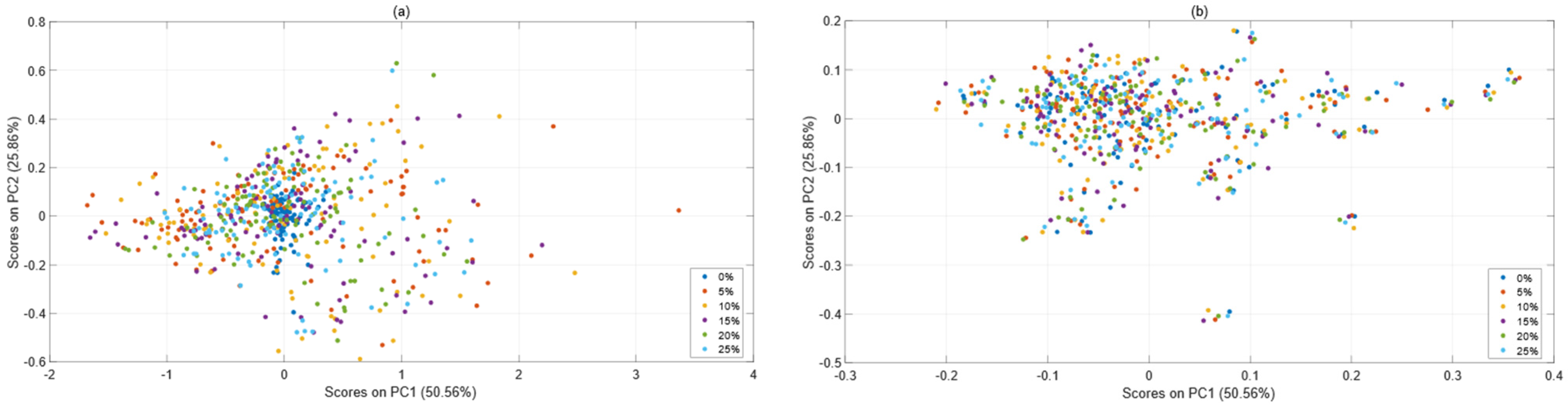
3.2. Comparison before and after Spectral Correction

Since S/B correction corrects TN prediction results according to the model rather than the spectral correction, the S/B correction method is not discussed here and is analyzed later. Figure 5 shows the six datasets’ spectra before and after the four methods for spectral correction of the effect of moisture. After SST correction (Figure 5b), the average spectral curves of soil samples with water contents of 5%, 10%, 15%, 20%, and 25% all overlapped with those of dry soil, indicating that the effect of moisture has been eliminated. After EPO correction (Figure 5e), the average spectral curves of soils with water contents of 5%, 10%, 15%, 20%, and 25% partially overlapped with those of dry soil, but the smoother spectra had errors. Overall, the difference between the spectral curves of wet and dry soils is significantly smaller, indicating that EPO can effectively eliminate the influence of moisture. After PDS and DS corrections (Figure 5d,e), the spectral differences between wet and dry soils were still prominent, and the noise contributed by moisture was not eliminated. Thus, SST has the best effect on mitigating the influence of moisture, followed by EPO, and PDS and DS have a poor effect.
After spectral correction, the distribution of soil spectra in the PC space with different water contents changed significantly. Before spectral correction, as shown in Figure 6a, the distributions of dry soils and wet soils are different on the PC1 axis. The distribution of scores for dry soils is concentrated and distributed in a narrow and extended area. The PCA score of wet soils has a slight overlap with those of dry soil, and mainly spreads along both sides of the PC1 axis to different degrees. After spectral correction using the SST method, as shown in Figure 6b, the score distribution of wet soils is consistent with the range of dry soils with only a minor deviation. The above results show that SST can effectively reduce the influence of moisture on the spatial score of soil spectral PCA. It is demonstrated that the SST method has a good effect in eliminating the influence of moisture on soil spectra.

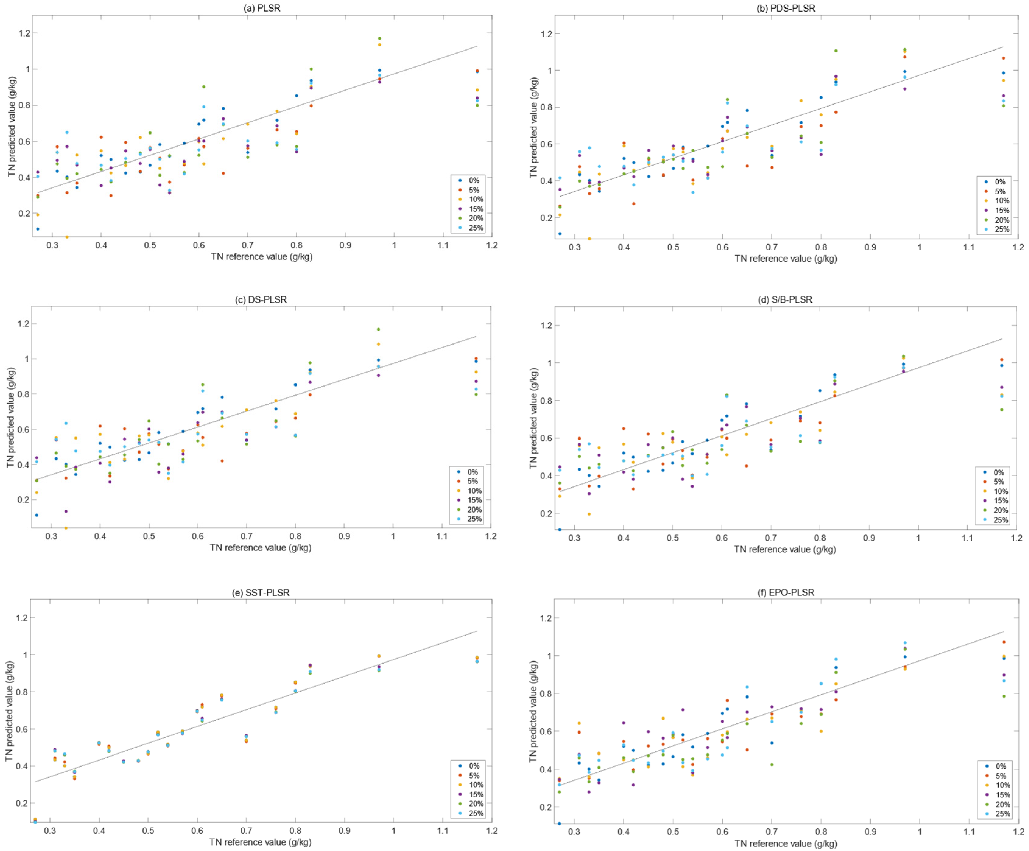
3.3. Comparison of Results of Different PLSR Models

3.3.1. PLSR Model for Dry Soil

Among all dry soil samples, 86 samples were selected to establish the PLSR model, and the others were used to validate the model. Table 2 shows the performance index information of the dry soil spectral PLSR model. The calibration set of soil spectra X and its corresponding true value of TN content Y are evaluated in the calibration step. The verification samples are considered to be an “unknown sample”, and the results obtained are as follows: calibration set: R c 2 = 0.74, RMSEC = 0.13g/kg; prediction set: R p 2 = 0.82, RMSEP = 0.09g/kg, RPD = 2.40. Since an RPD value greater than 2 represents good model performance, the established model can be considered good.

3.3.2. The Corrected PLSR Model

Table 2 shows that the use of the PLSR model is deplorable in predicting the spectra of wet soil samples. However, the accuracy of the wet soil model can be effectively improved by using the correction method. From the results, calibration and prediction effects of the SST–PLSR model are better than those of the PDS–PLSR, DS–PLSR, S/B–PLSR, and EPO–PLSR models. The results indicate that the performance of SST–PLSR is basically consistent with that of PLSR in dry soil, with R c 2 = 0.74, RMSEC = 0.13 g/kg, R p 2 in the range of 0.81~0.82, RMSEP in the range of 0.09~0.10 g/kg, and RPD in the range of 2.32~2.40 (Table 2). Compared with SST, EPO slightly improves the model but is better than PDS, DS, and S/B. The four correction methods of PDS, DS, S/B, and EPO could not maintain the same effect on the prediction model of TN content of wet soils under all different water contents, but SST could achieve similar effects.
In order to further explore the effect of SST on eliminating moisture’s effect on soil spectra, three comparisons were made in this paper: The first was to compare the TN prediction values of the PLSR model for soil samples under different water contents; the second was to compare the TN prediction values of PLSR, PDS–PLSR, DS–PLSR, S/B–PLSR, SST–PLSR, and EPO–PLSR; and the third was to compare TN prediction values of the same wet soil samples in PDS–PLSR, DS–PLSR, S/B–PLSR, SST–PLSR, and EPO–PLSR. As shown in Figure 7a, the prediction accuracy of the PLSR model is greatly affected by moisture. The predicted TN values across water contents and the TN content of dry soil samples were significantly different. There was a significant error between the predicted values of wet soil samples and the actual TN reference values (The TN reference values are the values obtained by the Kjeldahl method). However, after correction using PDS, DS, S/B, SST, and EPO methods (Figure 7b–f), the TN prediction accuracy of the corrected PLSR model for wet soil samples with different moisture contents was improved to varying degrees. Among these methods, the predicted values of TN for wet soil samples by SST–PLSR were consistent with the predicted values of dry soils regardless of the soil water content. Furthermore, the error between the predicted results of SST–PLSR and the relevant actual reference values was small. It has been proved that the prediction effect of SST–PLSR is better than those of other correction models.

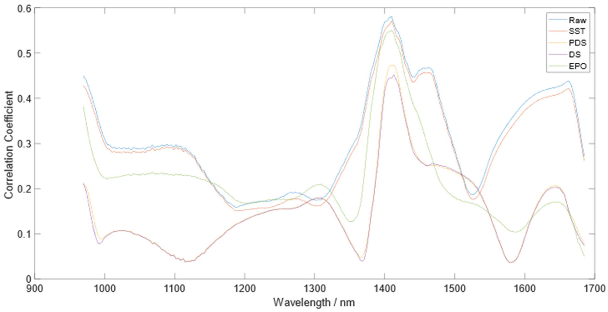
3.4. Correlation Coefficients between Dry Soil and Corrected Wet Soil and TN Content

Since the predictions of TN content are based on the entire NIR spectral range, it is necessary to evaluate the correlation coefficients between dry and corrected wet soil spectra and TN content. In general, the absolute value of the correlation coefficient in a particular spectral band is high, indicating that this band is an essential band for predicting TN content. Figure 8 shows the absolute value of the Pearson correlation coefficient between the soil spectra and the actual TN content, where the soil spectra include the dry soil spectra and the wet soil spectra corrected by PDS, DS, SST, and EPO. The dry soil spectra have the highest correlation coefficient with TN relative to the wet soil spectra. From the correlation coefficient curve of dry soil spectra and soil TN content, it can be seen that in the entire spectral range, the degree of correlation between the spectra of brick-red soil and TN is weak. However, the spectral band near 1400 nm (This band has the largest correlation coefficient value) has the most remarkable correlation, followed by the bands near 980 nm and 1650 nm, and the bands in other regions are less correlated. It is worth noting that the correlation coefficient between soil spectra and TN is not high for both dry and corrected wet soils, and the correlation is not improved after spectral correction. It can also be concluded from Figure 8 that the changes in the spectral and TN correlations of other wet soil samples after correction are similar to those of dry soil and TN. By comparing the correlation coefficient curves of all corrected wet soil spectra and soil TN, it can be found that the correlation between wet soil spectra after SST correction and TN is the closest to that of dry soil spectra and TN. This result further indicates that SST is the most effective method to eliminate the effect of moisture on soil spectra.

4. Discussion

A previous study [10] pointed out that only soil samples that have undergone a pretreatment operation of drying can obtain good model prediction results. In contrast, the model prediction errors of wet soil samples are large. This study also observed that prediction results of the PLSR model established with dry soil samples have little deviation from the actual values, as shown in Figure 7a. In this study, the prediction effect of dry soil samples for the PLSR model is good (RPD > 2), and RMSE is very low, around 0.1 g/kg. The established dry soil model can predict soil TN well. Although the RMSE is very low, the R 2 is not very high, which may be because the actual TN content range of the sample set is narrow and the content is low [29], resulting in low R 2 .
The change in the soil’s spectral reflectance curve is related to the changes in water content [8,14]. Since water molecules absorb across the entire spectral range, as the moisture content increased, the soil’s spectral reflectance showed an apparent decreasing trend (Figure 3), consistent with the results discovered by Li et al. [30,31]. When the water in the soil pores is saturated, it means that the soil water content reaches a critical value, and the influence of moisture on the spectra is maximized; if the water content exceeds the critical value, the water no longer has an impact on the spectra, and the reflectance of the whole spectra tends to be stable. The tipping point of soil moisture content depends on the soil type [32]. The strong absorption characteristic near the 1450 nm band is due to the adsorption of water and hydroxyl bonds (–OH) in the soil mineral surface and the 2:1 clay mineral structure [33], so the spectral curve changes most significantly around this band. The relationship between water content and spectral reflectance is often nonlinear [34]. This finding is consistent with previous findings [15,35].
As shown in Figure 8, the dry brick-red soil spectra and TN content showed a weak correlation. The most relevant spectral bands are around 1400 nm, followed by bands around 980 nm and 1650 nm. These influential bands (spectral bands with more excellent correlation) are usually related to C=O, C–H, O–H, and N–H bonds [30,34,36,37]. Generally speaking, soil’s spectral characteristics are a comprehensive reflection of soil’s physical and chemical characteristics. The correlation between spectral characteristics and TN is comprehensively affected by soil type, texture, organic matter, inorganic compounds, and background noise [38]. Several other organic/inorganic compounds have absorption characteristics in these spectral bands. Therefore, there are different critical bands for predicting TN content in different studies. However, the wet soil spectra were less correlated with TN than dry soils because the absorption characteristics of water molecules themselves would affect the degree of correlation between soil spectra and TN.
Because moisture significantly affects soil spectra, soil dryness seriously affects soil spectral prediction. To eliminate the interference caused by moisture and realize on-site spectral acquisition and analysis, researchers have proposed a variety of methods, among which the wet soil spectral correction method has been widely recognized [6,14,15]. Likewise, this study is also based on spectral correction. The purpose of wet soil spectral correction is to eliminate the influence of moisture. The corrected wet soil spectra can reflect the soil information more accurately. Five wet soil spectral correction methods have been executed, and the results show that SST is the best. SST can eliminate most of the effects of soil spectral reflectance changes caused by moisture, and after correcting the wet soil spectra, we obtain spectra consistent with dry soil samples (Figure 5). The tiny difference in the PCA score value projection map corresponding to the dry and SST-corrected wet soil spectra shows that SST can remove the difference between the dry and wet soils and ensure that the wet soils have a similar distribution area compared to the dry soils (Figure 6). It can also be observed by comparison with other correction methods that SST can preserve the correlation between spectral bands and TN to the greatest extent. Although EPO was considered to have the best effect on correcting wet soil spectra in previous studies [6,14], it can be seen from the above results that EPO still has apparent deviations, and it does not eliminate the noise caused by moisture. The deviation may be because EPO is not suitable for dealing with relatively smooth spectra. In addition, EPO assumes that the original spectral matrix of wet soils consists of three parts: a useful part related to soil properties, a part affected by moisture, and an independent residual part. However, in practical applications, the influence of the independent residual part is ignored [6], resulting in the deviation effect. PDS and DS correct the wet soil spectra based on the moving window method, which leads to a lack of spectral information [14]. From the results of spectral correction, their correction effect is poor since new noise is introduced. The S/B–PLSR model has the worst effect, probably because S/B is a linear correction for the predicted result values, and the effect of moisture on the soil spectra is nonlinear. In both the calibration set and prediction set, the RMSE of the wet soil sample model after SST correction is significantly reduced, the R 2 and RPD of the model are significantly improved, and the prediction results are almost the same as those of the dry soil samples. The evaluations in these aspects all prove that SST is the best spectral correction method to eliminate the influence of moisture.
In conclusion, the SST–PLSR model can be applied to the spectra of soil with different water contents. It is the best model used to correct the effect of soil moisture on near-infrared spectroscopy to predict total nitrogen in brick-red soil. By effectively eliminating the influence of moisture on spectra, SST–PLSR can obtain accurate prediction results using freshly collected wet soil samples. The method can be further extended to other types of soils, and can also be used to eliminate other environmental influences to achieve real-time analysis of soil nutrients in the field.

5. Conclusions

In this study, by analyzing the influence of moisture on the spectra of brick-red soil, it is found that moisture reduces the spectral reflectance and changes the distribution of the soil spectra PC space, thereby reducing the prediction accuracy of the model. Near-infrared spectroscopy combined with a spectral correction algorithm was used to eliminate the influence of moisture on the prediction of soil TN content, which increased the accuracy and robustness of the model. Among the five correction methods used, namely PDS, DS, S/B, SST, and EPO, SST showed the best results. All results of the SST–PLSR model, including the corrected spectral curve, principal component analysis scores, model evaluation indicators, predicted TN values, and important bands, proved that SST is the best methods to eliminate the influence of moisture on soil spectra. SST–PLSR is the best model used to correct the effect of soil moisture on NIR spectroscopy to predict total nitrogen in brick-red soils. SST can be applied to the prediction of different soil types and different soil nutrients to improve the robustness of the model. This technology provides new ideas for eliminating other environmental influences, supporting the development of soil field spectroscopy and portable spectrometers.

Author Contributions

Conceptualization, R.T. and J.W.; methodology, K.J., C.L. and X.L.; software, K.J.; writing—original draft preparation, R.T., K.J. and J.W.; writing—review and editing, R.T., K.J. and J.W.; supervision, C.L. and X.L. All authors have read and agreed to the published version of the manuscript.

Funding

This study was financially supported by the [innovative research team project of the Hainan Natural Science Foundation of China], funding number 320CXTD431; the [National Natural Science Foundation of China], funding number 32060413; and the [Hainan Graduate Innovation Research Fund], funding number No. Qhys2021-219.

Data Availability Statement

The data are not publicly available due to privacy.

Conflicts of Interest

The authors declare no competing interest.

References

  1. Ahrends, A.; Hollingsworth, P.M.; Ziegler, A.D.; Fox, J.M.; Chen, H.; Su, Y.; Xu, J. Current trends of rubber plantation expansion may threaten biodiversity and livelihoods. Glob. Environ. Chang. 2015, 34, 48–58. [Google Scholar] [CrossRef]
  2. Poorter, H.; Evans, J. Photosynthetic nitrogen-use efficiency of species that differ inherently in specific leaf area. Oecologia 1998, 116, 26–37. [Google Scholar] [CrossRef]
  3. Reddy, K.S.; Singh, M.; Tripathi, A.K.; Singh, M.; Saha, M.N. Changes in amount of organic and inorganic fractions of nitrogen in an Eutrochrept soil after long-term cropping with different fertilizer and organic manure inputs. J. Plant Nutr. Soil Sci. 2003, 166, 232–238. [Google Scholar] [CrossRef]
  4. Li, X.; Ge, T.; Chen, Z.; Wang, S.; Ou, X.; Wu, Y.; Chen, H.; Wu, J. Enhancement of soil carbon and nitrogen stocks by abiotic and microbial pathways in three rubber-based agroforestry systems in Southwest China. Land Degrad. Dev. 2020, 31, 2507–2515. [Google Scholar] [CrossRef]
  5. Etheridge, R.; Pesti, G.; Foster, E. A comparison of nitrogen values obtained utilizing the Kjeldahl nitrogen and Dumas combustion methodologies (Leco CNS 2000) on samples typical of an animal nutrition analytical laboratory. Anim. Feed. Sci. Technol. 1998, 73, 21–28. [Google Scholar] [CrossRef]
  6. de Santana, F.B.; de Giuseppe, L.O.; de Souza, A.M.; Poppi, R.J. Removing the moisture effect in soil organic matter determination using NIR spectroscopy and PLSR with external parameter orthogonalization. Microchem. J. 2018, 145, 1094–1101. [Google Scholar] [CrossRef]
  7. Cheng, H.; Wang, J.; Du, Y. Combining multivariate method and spectral variable selection for soil total nitrogen estimation by Vis–NIR spectroscopy. Arch. Agron. Soil Sci. 2020, 67, 1665–1678. [Google Scholar] [CrossRef]
  8. Zhou, P.; Yang, W.; Li, M.; Wang, W. A New Coupled Elimination Method of Soil Moisture and Particle Size Interferences on Predicting Soil Total Nitrogen Concentration through Discrete NIR Spectral Band Data. Remote. Sens. 2021, 13, 762. [Google Scholar] [CrossRef]
  9. Wang, W.; Yang, W.; Zhou, P.; Cui, Y.; Wang, D.; Li, M. Development and performance test of a vehicle-mounted total nitrogen content prediction system based on the fusion of near-infrared spectroscopy and image information. Comput. Electron. Agric. 2021, 192, 106613. [Google Scholar] [CrossRef]
  10. Tamburini, E.; Vincenzi, F.; Costa, S.; Mantovi, P.; Pedrini, P.; Castaldelli, G. Effects of Moisture and Particle Size on Quantitative Determination of Total Organic Carbon (TOC) in Soils Using Near-Infrared Spectroscopy. Sensors 2017, 17, 2366. [Google Scholar] [CrossRef] [Green Version]
  11. Stenberg, B. Effects of soil sample pretreatments and standardised rewetting as interacted with sand classes on Vis-NIR predictions of clay and soil organic carbon. Geoderma 2010, 158, 15–22. [Google Scholar] [CrossRef] [Green Version]
  12. Kuang, B.; Mouazen, A.M. Non-biased prediction of soil organic carbon and total nitrogen with vis–NIR spectroscopy, as affected by soil moisture content and texture. Biosyst. Eng. 2013, 114, 249–258. [Google Scholar] [CrossRef] [Green Version]
  13. Barthès, B.G.; Brunet, D.; Ferrer, H.; Chotte, J.-L.; Feller, C. Determination of Total Carbon and Nitrogen Content in a Range of Tropical Soils Using near Infrared Spectroscopy: Influence of Replication and Sample Grinding and Drying. J. Near Infrared Spectrosc. 2006, 14, 341–348. [Google Scholar] [CrossRef]
  14. Nawar, S.; Munnaf, M.A.; Mouazen, A.M. Machine Learning Based On-Line Prediction of Soil Organic Carbon after Removal of Soil Moisture Effect. Remote Sens. 2020, 12, 1308. [Google Scholar] [CrossRef] [Green Version]
  15. Wang, S.; Cheng, X.; Zheng, D.; Song, H.; Han, P.; Yuen, P. Application of Slope/Bias and Direct Standardization Algorithms to Correct the Effect of Soil Moisture for the Prediction of Soil Organic Matter Content Based on the Near Infrared Spectroscopy (English). Spectrosc. Spectr. Anal. 2019, 39, 1986–1992. [Google Scholar] [CrossRef]
  16. Jiang, Q.; Chen, Y.; Guo, L.; Fei, T.; Qi, K. Estimating Soil Organic Carbon of Cropland Soil at Different Levels of Soil Moisture Using VIS-NIR Spectroscopy. Remote. Sens. 2016, 8, 755. [Google Scholar] [CrossRef] [Green Version]
  17. Liu, Z.-P.; Shao, M.-A.; Wang, Y.-Q. Spatial patterns of soil total nitrogen and soil total phosphorus across the entire Loess Plateau region of China. Geoderma 2013, 197–198, 67–78. [Google Scholar] [CrossRef]
  18. Chu, X.L.; Yuan, H.F.; Lu, W.Z. Model Transfer in Multivariate CalibrationModel Transfer in Spectral Multivariate Correction. Spectrosc. Spectr. Anal. 2001, 21, 881–885. [Google Scholar] [CrossRef]
  19. Liu, Y.; Deng, C.; Lu, Y.; Shen, Q.; Zhao, H.; Tao, Y.; Pan, X. Evaluating the characteristics of soil vis-NIR spectra after the removal of moisture effect using external parameter orthogonalization. Geoderma 2020, 376, 114568. [Google Scholar] [CrossRef]
  20. Du, W.; Chen, Z.-P.; Zhong, L.-J.; Wang, S.-X.; Yu, R.-Q.; Nordon, A.; Littlejohn, D.; Holden, M. Maintaining the predictive abilities of multivariate calibration models by spectral space transformation. Anal. Chim. Acta 2011, 690, 64–70. [Google Scholar] [CrossRef]
  21. Rehman, T.U.; Zhang, L.; Ma, D.; Wang, L.; Jin, J. Calibration transfer across multiple hyperspectral imaging-based plant phenotyping systems: I-Spectral space adjustment. Comput. Electron. Agric. 2020, 176, 105685. [Google Scholar] [CrossRef]
  22. Li, J.; Zhou, L.; Lin, W. Calla lily intercropping in rubber tree plantations changes the nutrient content, microbial abundance, and enzyme activity of both rhizosphere and non-rhizosphere soil and calla lily growth. Ind. Crop. Prod. 2019, 132, 344–351. [Google Scholar] [CrossRef]
  23. Bremner, J.M. Determination of nitrogen in soil by the Kjeldahl method. J. Agric. Sci. 1960, 55, 11–33. [Google Scholar] [CrossRef]
  24. Nawar, S.; Mouazen, A. On-line vis-NIR spectroscopy prediction of soil organic carbon using machine learning. Soil Tillage Res. 2019, 190, 120–127. [Google Scholar] [CrossRef]
  25. Xu, Z.; Fan, S.; Liu, J.; Liu, B.; Tao, L.; Wu, J.; Hu, S.; Zhao, L.; Wang, Q.; Wu, Y. A calibration transfer optimized single kernel near-infrared spectroscopic method. Spectrochim. Acta Mol. Biomol. Spectrosc. 2019, 220, 117098. [Google Scholar] [CrossRef] [PubMed]
  26. Fonollosa, J.; Fernández, L.; Gutiérrez-Gálvez, A.; Huerta, R.; Marco, S. Calibration transfer and drift counteraction in chemical sensor arrays using Direct Standardization. Sensors Actuators Chem. 2016, 236, 1044–1053. [Google Scholar] [CrossRef] [Green Version]
  27. Hu, B.; Chen, S.; Hu, J.; Xia, F.; Xu, J.; Li, Y.; Shi, Z. Application of portable XRF and VNIR sensors for rapid assessment of soil heavy metal pollution. PLoS ONE 2017, 12, e0172438. [Google Scholar] [CrossRef] [Green Version]
  28. Chang, C.-W.; Laird, D.A.; Mausbach, M.J.; Hurburgh, C.R., Jr. Near-Infrared Reflectance Spectroscopy-Principal Components Regression Analyses of Soil Properties. Soil Sci. Soc. Am. J. 2001, 65, 480–490. [Google Scholar] [CrossRef] [Green Version]
  29. Kuang, B.; Mouazen, A.M. Calibration of visible and near infrared spectroscopy for soil analysis at the field scale on three European farms. Eur. J. Soil Sci. 2011, 62, 629–636. [Google Scholar] [CrossRef]
  30. Mouazen, A.M.; De Baerdemaeker, J.; Ramon, H. Towards development of on-line soil moisture content sensor using a fibre-type NIR spectrophotometer. Soil Tillage Res. 2005, 80, 171–183. [Google Scholar] [CrossRef]
  31. Li, S.; Shi, Z.; Chen, S.; Ji, W.; Zhou, L.; Yu, W.; Webster, R. In Situ Measurements of Organic Carbon in Soil Profiles Using vis-NIR Spectroscopy on the Qinghai–Tibet Plateau. Environ. Sci. Technol. 2015, 49, 4980–4987. [Google Scholar] [CrossRef] [PubMed]
  32. Lobell, D.B.; Asner, G.P. Moisture Effects on Soil Reflectance. Soil Sci. Soc. Am. J. 2002, 66, 722–727. [Google Scholar] [CrossRef]
  33. Viscarra Rossel, R.A.; Behrens, T.; Ben-Dor, E.; Brown, D.J.; Demattê, J.A.M.; Shepherd, K.D.; Shi, Z.; Stenberg, B.; Stevens, A.; Adamchuk, V.; et al. A global spectral library to characterize the world’s soil. Earth Sci. Rev. 2016, 155, 198–230. [Google Scholar] [CrossRef] [Green Version]
  34. Xu, S.; Zhao, Y.; Wang, M.; Shi, X. Comparison of multivariate methods for estimating selected soil properties from intact soil cores of paddy fields by Vis–NIR spectroscopy. Geoderma 2018, 310, 29–43. [Google Scholar] [CrossRef]
  35. Cao, Y.; Bao, N.; Liu, S.; Zhao, W.; Li, S. Reducing moisture effects on soil organic carbon content prediction in visible and near-infrared spectra with an external parameter othogonalization algorithm. Can. J. Soil Sci. 2020, 100, 253–262. [Google Scholar] [CrossRef]
  36. Rossel, R.V.; Cattle, S.; Ortega, A.; Fouad, Y. In situ measurements of soil colour, mineral composition and clay content by vis–NIR spectroscopy. Geoderma 2009, 150, 253–266. [Google Scholar] [CrossRef]
  37. Stenberg, B.; Viscarra-Rossel, R.A.; Mouazen, A.M.; Wetterlind, J. Visible and Near Infrared Spectroscopy in Soil Science. Adv. Agron. 2010, 107, 163–215. [Google Scholar] [CrossRef] [Green Version]
  38. Li, M.; Zheng, L.; An, X.; Sun, H. Fast Measurement and Advanced Sensors of Soil Parameters with NIR Spectroscopy. J. Agric. Mach. 2013, 44, 73–87. [Google Scholar] [CrossRef]
Figure 1. Location of the study area and spatial pattern of soil sampling in Danzhou City, Hainan Province, China.
Electronics 12 01271 g001
Figure 2. The flowchart illustrates the different steps performed during model calibration and wet and dry soil spectral data validation.
Electronics 12 01271 g002
Figure 3. (a) Average spectral reflectance of soil samples with moisture contents of 0% (dry soil), 5%, 10%, 15%, 20%, and 25%; (b) the difference spectra of the wet soil samples with water contents of 5%, 10%, 15%, 20%, and 25% and the dry soil sample.
Electronics 12 01271 g003
Figure 4. PC1 and PC2 scores after PCA for soil spectra at 0% (dry soil), 5%, 10%, 15%, 20%, and 25% moisture content.
Electronics 12 01271 g004
Figure 5. Average spectral curves of soil samples with 0% (dry soil), 5%, 10%, 15%, 20%, and 25% moisture content: (a) before spectral correction, (b) after SST correction, (c) after PDS correction, (d) after DS correction, (e) after EPO correction.
Electronics 12 01271 g005aElectronics 12 01271 g005b
Figure 6. Distribution of PCA score values for soils with 0% (dry soil), 5%, 10%, 15%, 20%, and 25% moisture content (a) before and (b) after SST correction.
Electronics 12 01271 g006
Figure 7. Comparison of reference values (the values of TN content obtained by the Kjeldahl method) for soil TN content with model-validated predictions using different models for soils with 0% (dry soil), 5%, 10%, 15%, 20%, and 25% moisture content: (a) PLSR, (b) PDS–PLSR, (c) DS–PLSR, (d) S/B–PLSR, (e) SST–PLSR, (f) EPO–PLSR.
Electronics 12 01271 g007
Figure 8. The correlation coefficient between the soil spectra and the TN content in all wavelengths.
Electronics 12 01271 g008
Table 1. Descriptive statistical characteristics of soil TN content.
Type of
Samples
Number of
Samples
MaxMinMeanMedianStandard
Deviation
TN (g/kg)Total
samples
1071.740.130.580.530.25
Calibration samples861.740.130.580.530.25
Prediction samples211.170.270.580.540.23
Notes: TN, total content; Max, maximum; Min, minimum.
Table 2. TN prediction results of PLSR model under dry soil spectra and corrected PLSR model under wet soil spectra.
ModelMoisture
Content %
Calibration SetPrediction Set
R c 2 RMSEC (g/kg)RPD R p 2 RMSEP (g/kg)RPD
PLSR00.740.131.710.820.092.40
PLSR5–250.38–0.700.15–0.200.80–1.550.49–0.680.13–0.171.43–1.80
SST–PLSR5–250.740.131.710.81–0.820.09–0.102.32–2.40
EPO–PLSR5–250.65–0.710.14–0.151.40–1.610.69–0.780.10–0.121.84–2.17
PDS–PLSR5–250.43–0.660.14–0.190.93–1.410.52–0.740.11–0.151.46–2.02
DS–PLSR5–250.43–0.690.14–0.190.93–1.450.50–0.700.12–0.161.45–1.89
S/B–PLSR5–250.42–0.660.14–0.190.92–1.410.55–0.690.12–0.151.53–1.86
Notes: the values in bold in Table 2 are the metric values for the best correction model.
Disclaimer/Publisher’s Note: The statements, opinions and data contained in all publications are solely those of the individual author(s) and contributor(s) and not of MDPI and/or the editor(s). MDPI and/or the editor(s) disclaim responsibility for any injury to people or property resulting from any ideas, methods, instructions or products referred to in the content.

