1. Introduction
Nowadays, various machine learning methods provide excellent results in different classification and object recognition tasks. These methods reach or even exceed the performance of humans in numerous cases. One of the examples is the best-performing model on the Modified National Institute of Standards and Technology (MNIST) dataset [
1], achieving an error rate of 0.21% [
2]. Based on these impressive achievements, this field no longer contains challenges. However, the experiments yielding these results were conducted in closed-set scenarios, assuming that all possibly occurring classes are known during the training phase of the models. The open-set case is a much more realistic scenario, where new classes can appear after optimizing the model’s parameters. Hence, during the evaluation of the method, the data samples belonging to previously unknown classes must be rejected. Traditional recognition algorithms fail to solve the task even if the dataset is precisely classified in a closed-set setting.
In this study, we abandoned the idea of partitioning the space of data (or features) with hyperplanes because most of the possible inputs are not part of any known classes. Instead, this approach is a distance-based method. In essence, the output of our model is a feature space instead of the logit space. This space has low dimensions and is constructed to fulfill the following requirements: samples of the same class lie near each other, while samples of different classes are far from each other.
Based on experimental results, we found that it is advantageous to have fixed class centers for using pairwise distances, and the model cannot reliably accumulate all the samples of a class into one area of the feature space. The experiments also showed the necessity of using generated data to represent the intraclass space to optimize the parameters; otherwise, the model contracts the whole input space around the class centers. In this way, the open-set recognition (OSR) problem becomes determining to how to create the appropriate synthetic data samples for the training of the model.
However, generating fake inputs of appropriate quality is a challenging task for a reason more deeply explained in this paper. Moreover, creating and using these samples increases computational costs at two stages of the procedure: First, one must train the generative model, which is computationally expensive if the goal is to create high-quality data. Second, the generated samples must also be run through the classifier.
We thus generated fake features using the features of real data in a hidden layer of an artificial neural network to consistently achieve better results. As the samples classified in this study are image datasets, the backbone of the model is a convolutional neural network. It is built from several convolutional layers, followed by a few fully connected ones. The experiments showed that after all the convolutional layers, generating the features in a hidden layer is optimal in the later components of the model. The much simpler structure of this layer enables the use of a significantly smaller generative model. At the same time, the generated samples have to be run only through the second, a minor part of the classifier. In this way, the further computational costs caused by using synthetic samples are almost entirely eliminated.
The paper is structured as follows: After a brief overview of the related work, we introduce our approach in detail and present the experimental performance results by comparing them to the performance of other existing methods in various OSR scenarios. A detailed analysis of runtimes is also provided, comparing the phases of the model and the models generating features and images.
2. Literature Review
In this section, we briefly review the corresponding literature, beginning with the theory of open-set recognition, then continuing with the most relevant solutions.
2.1. Theory of Open-Set Recognition
Many algorithms have long been used to solve classification tasks where only some samples belong to any known class [
1,
3] or the machine needs to be more confident [
4,
5] in classifying. The formalization of the theory of open-set recognition was introduced by Scheirer et al. [
6]. We follow their definitions.
Let
O denote the open space (i.e., the space far from any known data). The open space Rrsk is defined as follows
where
denotes the space containing both the positive training examples and the positively labeled open space, and
f is the recognition function, with
if the sample
x is recognized as as a known class and
otherwise.
Definition 1. Open-Set Recognition Problem: Let V be the set of training samples, be the open space risk, and be the empirical risk (i.e., the closed set classification risk, associated with misclassifications). Then, open-set recognition is the task of finding an measurable recognition function, where means classification into a known class, and f minimizes the open-set risk: where is a regularization parameter balancing open space risk and empirical risk. Definition 2. The openness of an open-set recognition problem is defined as follows (according to [6]):where denote the training, target, and test classes, respectively. Extreme Value Theory
SVMs and SoftMax classifiers were initially designed for the closed-set scenario and have been modified to reject open-set samples to some extent. Another example is OpenMax by Bendale et al. [
7], who changed a neural network classifier after being first trained in the traditional closed set scenario with a SoftMax layer. However, to achieve better results, the principle of dividing the input/feature space with hyperplanes or otherwise has to be revised, and fundamentally different approaches are needed.
The probability of a sample belonging to a given class can be statistically approached by considering the distribution of distances from the training samples in feature space.
Jain et al. [
8] set a solid theoretical base, extreme value theory (EVT), showing the connection between the probability of a sample belonging to a class and the distance of the sample from the known (training samples). Extreme value machine (EVM) directly applies the margin distribution theorem. After fitting a Weibull distribution on each training instance in the feature space, the model is reduced: instances covered by other instances with high probability are discarded. The remaining ones become extreme vectors. EVM is a computationally cheap and fast model. However, extracting appropriate features from the data is not a part of it, which is a severe limitation. The features have to be extracted before applying the model. Descriptors have been used for the tests on image datasets, but these are inferior to the state-of-the-art convolutional networks. Additionally, using these convolutional networks nullifies this model’s main advantage: its extremely low complexity.
Extreme value theory is used in various other open-set recognition methods. Jain et al. [
9] introduced
-SVM to estimate the posterior probability of class inclusion. They used EVT on the pretrained 1-vs-Rest RBF SVM output values to obtain the unnormalized posterior probability. The modification, which Bendale et al. used to create OpenMax, is also based on EVT [
7].
2.2. Distance-Based Methods
Distance-based methods inherently fit into the open-set scenario. In addition to deciding which class is the most similar to the sample in question, they provide a value on the extent of the similarity. Using this value, e.g., applying a threshold on it, one can decide whether the sample belongs to the most similar class or is unknown.
Júnior et al. [
10] extended the nearest neighbor classifier to the open-set scenario. To decide where sample
s belongs, its nearest neighbor
t is first taken, then the nearest neighbor
u s.t.
u and
t are of different classes. If the ratio of the distances
is less than a threshold
T,
s is classified with the same label as
t; otherwise, it is rejected as unknown.
Instead of using the distances between individual instances, Miller et al. [
11] used predefined (so-called anchored) class means. A network projects each input into the logit space. Then, the decision is made according to the Euclidean distances between the logit vectors and the class means.
Sample Generation
The biggest issue with open-set recognition is that the model cannot be trained, and samples have to be rejected, as unknown classes occur only during tests. Using generated data to model these samples can improve the performance of an open-set classifier.
Generative adversarial network (GAN) was created by Goodfellow et al. [
12]. It is a method capable of generating images similar to the real ones. It is made of two separate neural networks. One is trained to generate fake data from the noise to deceive the other; the other is trained to separate the actual images from those generated by the first network.
Kong and Ramanan [
13] created a version of GAN that generates fake images that is capable of improving the performance of OSR. They supplemented the GAN model with feature vectors for conditioning. Our solution—namely, that we generate inner features instead of images—does not require additional conditioning, making both the training of the GAN model and using the generated samples computationally much more efficient while equallycontributing to the performance of the OSR model. Other solutions, such as those of Jo et al. or Ge et al. [
14,
15], have used GANs as well. Another method to generate samples is the usage of autoencoders [
16]. In one solution [
17], autoencoders were used for the classification itself, with the reconstruction error being the base of the decision. Generating negative samples can significantly improve the performance of an OSR model. However, their significant extra computational cost is a major drawback.
3. Proposed Novel Approach
Neural-network-based methods are the most popular and some of the most successful tools for classification tasks. However, adapting them to the open-set scenario is still challenging, considering the SoftMax layer used on these networks. We present a different approach. Instead of applying a SoftMax layer (and thus dividing the state space with hyperplanes), the output of the network is a space in which the distance is minimal if the samples x and y belong to the same class and are maximal otherwise. is the output of the network on the input x. Algorithm 1 shows the proposed model. We are describing its details below.
3.1. Fixed Class Centers
It is simpler to use fixed class centers instead of pairwise distances, as was reported in [
11]. Hence, there is no need to either explicitly motivate the different classes to be far from each other or to calculate the pairwise distances; the training is thus simplified into a quadratic regression: let
be the class centers for the
k known classes. Then, the loss function for
, where
x is a sample from class
i, is simply
. The class centres are one-hot vectors and their opposites:
,
,
, etc.; the dimension of the output space is thus
. Using the opposites of one-hot vectors makes the origin the average output and, statistically, the expected value when encountering new samples.
3.2. Sample Generation
To improve the ability of the model to recognize unknown inputs, synthetic data are used to model the space of these unknowns during training. The samples are obtained by a generative adversarial network [
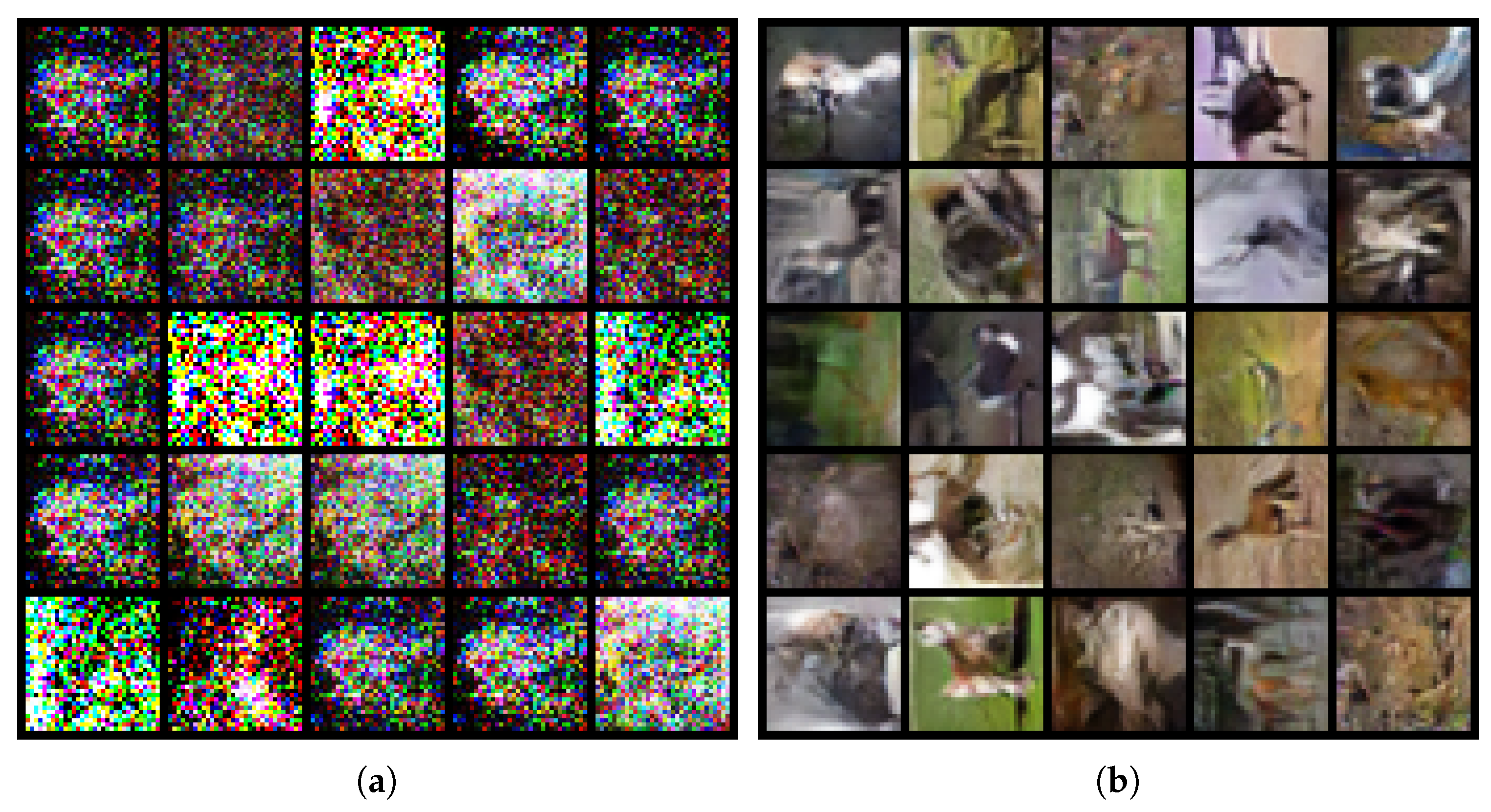
12]. The samples to train it are positive training inputs. However, the experiments showed that generating appropriate fake images is a challenging task. Using a too-simple model results in low-quality images. Although the model can easily be trained to reject them, training does not sufficiently prepare the model to reject real unknown samples. With a more complex model, we could generate high-quality images; however, training the model to reject these led to the rejection of unseen test samples of known classes.
Figure 1 illustrates the two extreme cases. We were unable to reliably find the optimal middle ground.
Hence, the synthetic samples are generated in a hidden feature layer instead of the input space. This requires the real features from this layer. These are accessible by dividing the neural network model into two parts: and . is responsible for the feature extraction, and transforms the features into the output space. Let be the function implemented by ; similarly, let be the function implemented by . Then, feeding with the outputs of and training the system with the above-described loss function gives . Extensive experiments were conducted across various datasets to find the best cutting point of the model. Through these experiments, we empirically proved that cutting the model after all the convolutional layers provides us with the optimal middle ground mentioned before.
Using this setup, the training process is as follows: First, the networks are pretrained on the set of real images
to implement
. Then, the features
are saved. These features are used to train the generative model and to further train
on these features and on the synthetic ones.
is not trained anymore or used during the training anymore. This greatly decreases the computational costs of the second phase of the training in light of this being part of the model with the convolutional layers; thus, this is the most expensive one to run. The features
are utilized as real data to train the generator
and discriminator
models using the algorithm described by [
12]. After training,
creates the synthetic features
from random noise
z of the same distribution
used by training the GAN. These fake features are then used alongside the real features
to further train
. The loss function is the same for the known features:
, where
is the predefined class center of class
i of sample
x. The goal of regression for the fake features is the origin; the loss function is thus
.
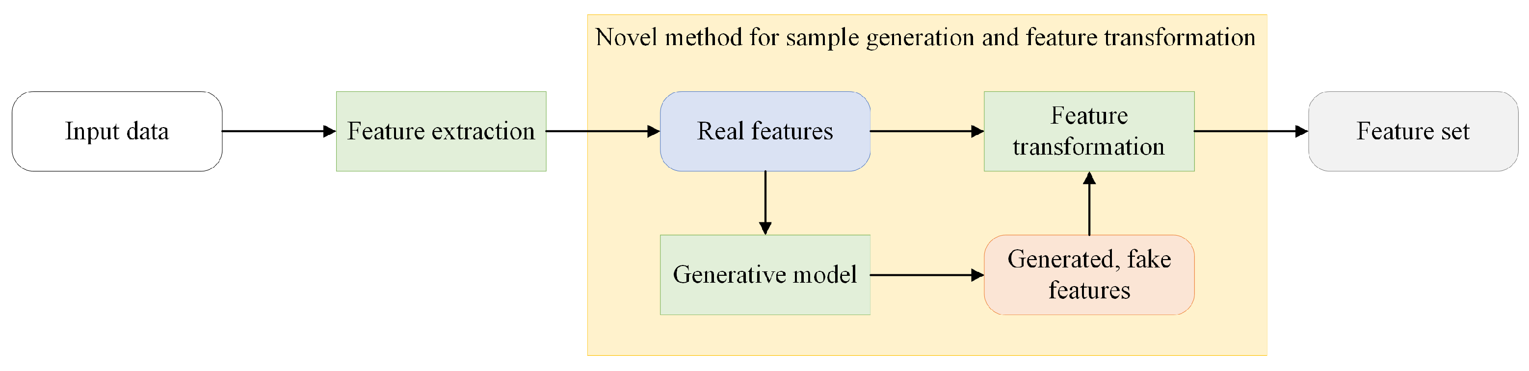
Figure 2 shows a schematic representation of the algorithm.
4. Experimental Results
We evaluated the performance of our method by comparing it to other relevant methods and a baseline, which was equivalent to our model but without the use of generated negative inputs.
4.1. Implementation Details
As the backbone of the model, different-sized versions of VGGNet were used depending on the size and complexity of the images in the datasets [
18]. The convolutional layers, including the max pooling after the last convolutional layer, form the first part of the model. The second part follows the fully connected layers of the same network, e.g., when using VGG19 as the backbone. The second part consists of three hidden layers of 4096, 4096, and 1000 neurons with ReLU as the activation function. The output is a linear layer with several neurons equal to half of the training classes.
Using the generative model in the feature layers enables both the Generator and the Discriminator to be simple, fully connected networks. The Generator consists of two 256-neuron and two 512-neuron linear hidden layers. The input layer has a dimension of 128, i.e., the Generator takes 128-dimensional random vectors as input. The dimension of the output is equal to the dimension of the output of
. The Discriminator is symmetrical to the Generator: it has two 512-neuron and two 256-neuron hidden layers, this time completed with LeakyReLU, and the output is a single neuron with sigmoid activation. For training, an Adam optimizer [
19] was used with a base learning rate of
,
,
and a batch size of 64.
4.2. Datasets
We compared some of the most common datasets and experimental setups listed below.
The Street View House Numbers (SVHN) dataset consists of
images of digits cropped from house number plates [
20]. It is considered an easy-to-classify dataset: the accuracy of the best-performing models in closed-set scenarios approaches 99%.
The CIFAR-10 (Canadian Institute For Advanced Research) [
21] dataset, on the other hand, is slightly more challenging. However, it has the same size in terms of individual images and the number of classes. It consists of
natural images of ten classes, six of which are different animals, with the remaining four being various vehicles.
For both CIFAR-10 and SVHN, six out of ten classes served as known classes with positive samples; the remaining four provided the unknown samples. The openness of these problems is
, following Equation (
3). The backbone of the model was VGG13 in the case of CIFAR-10 and VGG11 in the case of SVHN.
TinyImageNet is a dataset similar to ImageNet; one can consider it a downscaled version. The images are smaller () and contain 200 classes with 500 training images each. The model was trained on only 20 classes from this dataset, and the remaining 180 were used as unknown, resulting in an openness value of . This time, the backbone network was VGG16.
CIFAR+10 and CIFAR+50 involved training the model on four classes from CIFAR-10 and using 10 and 50 nonoverlapping classes, respectively, from CIFAR-100 as unknowns, with the openness of and , respectively, using VGG13 as in the CIFAR-10 6 + 4 scenario.
In addition to the previously described open-set scenarios, a test on outlier detection was also conducted, following the protocol defined by [
22]: we trained the model on all ten classes of CIFAR-10 and tested it on outliers from the ImageNet and LSUN datasets obtained by [
23].
Each test was repeated ten times, and the results were averaged, although the deviation of the values was negligible. Random class splits were used (in the case of CIFAR+10 and CIFAR+50 with the described constraints), except for the test on outliers (
Table 1), where the protocol strictly specifies the classes used for training.
We also analyzed time complexity, comparing the runtime of a batch on the two parts of the model and the time needed for an iteration on a batch with our generative model and with one that would generate synthetic images.
4.3. Evaluation Metrics
According to a thorough survey on OSR methods by Geng et al., the most common metrics for evaluating open-set performance are AUC and F1 measure [
24]. In terms of overall accuracy or F1 measure, the metric is highly sensitive to its calibration, in addition to the real effectiveness of a model [
25]. Hence, we evaluated open-set recognition performance with the two metrics described below. The F1 measure was still used to assess performance on the above-described outlier detection, as the other results obtained, followed by the protocol, were also published in this metric. In this case, cross-class validation is used to estimate the difference between the optimal thresholds of the training set—where the positive samples are the positive training samples, and the negative samples are the generated ones—and the test set.
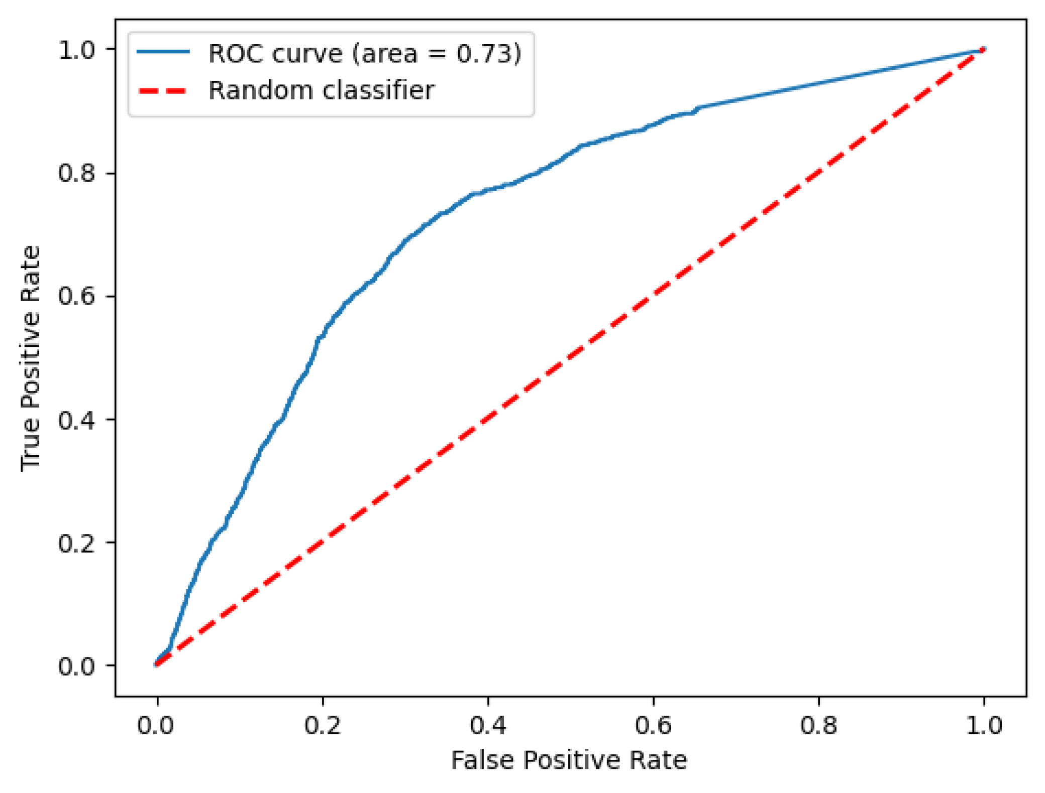
AUC: The receiver operating characteristic (ROC) curve is obtained by plotting the true positive rate (sensitivity) against the false positive rating (1 –specificity) at every relevant threshold setting. The area under this curve gives a calibration-free measure of the open-set detection performance [
26].
Closed set accuracy: It is essential that the model, while being able to reject unknown samples, retains its closed-set performance. Therefore, the closed-set accuracy on the test samples of known classes was also measured.
4.4. Results
Table 2 shows the open-set detection performance of the baseline, proposed method, and other approaches in terms of AUC value. The ROC curve in the case of TinyImageNet can be seen in
Figure 3.
We employed the same model structure as another comparison base to classify the same inputs. However, without using generated samples, the training was identical to Algorithm 1 to line 10, with the number of iterations
being higher. This method is referred to as a baseline in the tables. Our approach outperforms the baseline and most other listed methods on TinyImageNet, practically tying for first place. At the same time, CIFAR-10 performed the best by a large margin. On SVHN, however, it performed significantly worse. The pattern is clear: our model achieved the best relative performance on the more difficult-to-classify natural images: TinyImageNet is far larger than the others, both in terms of the number of categories and the size of the images. CIFAR-10 is smaller but famously difficult to accurately classify compared with its size. This is exactly the opposite of the result of Neal et al. Their approach worked exceptionally well on SVHN or MNIST. Still, the model’s performance significantly dropped on natural images such as CIFAR or TinyImageNet. In the case of CIFAR+ scenarios, the method by [
11] outperformed the other methods, but all others produced similar, reasonably good performance, including ours [
27].
| Algorithm 1 The training procedure of the model |
- Require:
training samples, numbers of iterations - Output:
Neural network models and fixed class centers - 1:
Initialize with random parameters, class centers - 2:
- 3:
- 4:
fordo - 5:
for j in batches do - 6:
- 7:
- 8:
Update and with the gradient of the loss - 9:
end for - 10:
end for - 11:
- 12:
- 13:
z← random noise - 14:
- 15:
fordo - 16:
for j in batches do - 17:
- 18:
- 19:
- 20:
- 21:
Update with the gradient of the loss - 22:
end for - 23:
end for - 24:
return
|
The closed-set accuracy values are shown in
Table 3. No information on the other methods’ performance on TinyImageNet was available regarding this measure; hence, we could compare our result only to our baseline. However, our open-set recognition method fully retains its closed-set accuracy; on CIFAR-10 and SVHN, the accuracy even increases when using the generated samples; on CIFAR-10, the difference is significant. Our closed-set accuracy is also superior to that of the other published methods, but with a slight difference on CIFAR-10.
The results of the tests on various outliers are presented in terms of macro-averaged F1 measure (
Table 1) to compare them to the results obtained with other methods, which were also published using this metric. However, this metric does not show if the method produces better closed-set accuracy with inferior open-set detection or vice versa. Hence, we considered it proper to analyze and present the AUC and closed-set accuracy as well. The closed-set accuracy was 0.912, on average, on all ten classes of CIFAR-10, which is similar to the value of
on the six known classes of the 6+4 open-set scenario. The average AUC varied between 0.893 and 0.903 across the four categories of outliers. Regarding the F1 measure, our model performed best in two outlier categories, reaching second and third place in the other two, trailing slightly behind the best-performing models. The standard deviation of the results was very low in every case. The nature of the model—the training is simplified to a quadratic regression with fixed class centers—makes it remarkably stable. Only the choice of known or unknown classes slightly varies the results.
4.5. Large-Scale Test on ImageNet
To validate that the model scales well on datasets greater in size and variability, it was tested on the ImageNet (ILSVRC-2012) dataset [
29]. Although the existing OSR models were not tested on it by the authors, we could compare the results to the ones on other datasets, for example, the similar TinyImageNet, as well as to the accuracy of the closed-set model VGG19 [
18]. For the training, the same network structure was used as for TinyImageNet. The hyperparameters also followed the tests on the other datasets. The results are shown in
Table 4.
Both the AUC and accuracy values showed only a minor decrease when there were more than 40 training classes, which showed that the model scales well with the size of the problem. Additionally, note that when training on 20 classes, the results were significantly better than those on TinyImageNet, where 20 known classes were used as well, but the images were smaller. This means that the model can utilize the more detail provided by the bigger images of ImageNet.
We also measured the change in the AUC value when varying the number of unknown classes. The model trained on 150 known classes was used. The results are shown in
Table 5.
The results were approximately the same regardless of the number of unknown classes, with the only deviance being higher with fewer unknown classes. This shows the strength of the AUC measure, as it is independent of the threshold and the ratio of the positive and negative samples. When testing on a subset of unknown classes, the result varied depending on how hard-to-reject classes are chosen, but the expected value was the same as when testing on all the classes.
4.6. Time Complexity Analysis
Generating samples in an inner layer, in addition to producing better performance in terms of accuracy, results in computationally cheaper training than with generating synthetic inputs. This advantage appears at two distinct points. First, during the training, both the generative and discriminative networks are smaller and of a more straightforward structure than what would be needed for generating images. Second, as the generated samples are already in the hidden layer, during the further training of the model, these samples do not have to be run through the first part of the model. Hence, by saving the output of the model’s first part on the real training samples, there is no need to use this first part for the second training phase.
To measure the time-complexity gain, we obtained measures on runtimes. All the measurements were obtained on the same architecture:
To estimate how the time-gain scaled on real-life (most likely higher resolution) datasets, the measurements were obtained on all three primary datasets used for the experiments.
Table 6 shows the runtimes of the training of the different types of GAN-s.
The values are the runtimes of a training step—running the models, calculating the gradients, and adjusting the weights—on a batch of 64 samples, measured in milliseconds. The difference between the training of the generative models is 3–4 fold on the smaller datasets but exceeds an order of magnitude on TinyImageNet. This led to the conclusion that the time gain achieved by our method is more significant on larger, real-life datasets. The experiments showed that no more iterations are needed to generate appropriate features than to generate images of sufficient quality. Hence, these ratios are the actual gain on the generative part of the training.
We measured the time needed to run a batch of 64 samples through the two parts of the model. The results are also shown in milliseconds in
Table 7.
The last row is the ratio of the sum of runtimes and the runtime of the second part, as a generated feature has to be run only on the second part, while a generated (or real) image has to be run through the whole model. For the different datasets, differently sized model structures were used, corresponding to the sizes and difficulties of images. This significantly altered the results between the datasets. It is clear that as the size of the problem scales up, the ratio improves, exactly as in the training of the generative model.
The times needed for a whole training step, also including the calculation of gradients and making the training step, with generated features (only the second part of the model) or with images (the whole model) are shown in
Table 8.
The ratios show a similar pattern to the raw runtime of the model parts. However, they are slightly smaller because a training iteration has some operations that do not scale up with the model’s size.
During the experiments, it proved to be optimal to have generated samples in an equal number to all real samples. Considering this, using the synthetic features, the whole training required barely more than half as long as using the generated images—the exact ratio was on TinyImageNet—even if both the phases by one are as long in terms of iterations as the whole training with generated images.
5. Conclusions
Open-set recognition faces a new, more complex challenge than the closed-set scenario when all classes are known at training time. Modeling the space of possible unknowns by generating artificial samples was proven to help solve this issue. However, creating and using these samples induce further computational costs.
By using generated features in an inner layer of the model, we made progress both in terms of performance and computational efficiency. Apart from beating the baseline—an identical model without using fake features—our approach performed better than most of the other methods, even with this otherwise elementary model. While generalizing to be able to reject open samples, the model also retains its closed-set accuracy. Up to 150 known classes, the accuracy only dropped down to 75.2%. As a comparison, the classical, closed-set VGG19 network performed 72.7% on all 1000 classes of ImageNet. On two out of the three other datasets, our model outperformed the baseline, which is a closed-set model.
As tests on the ImageNet dataset showed, the model scales well with the size of the problem. When the number of training classes was comparable to the known classes of TinyImageNet, the results were better than on TinyImageNet. This means that the model benefited from more detail because ImageNet has bigger images ( instead of ), which showed that the model retained its strength in feature extraction.
Meanwhile, the computational cost induced by generating and using samples is practically eliminated: On TinyImageNet, generating synthetic inputs took 11 times more time than generating features. While using them for training, the difference was more than seven-fold.
One limitation of the model presented in this paper is that the approach was applied to simpler backbone models. Therefore, its full potential has not yet been used. Applying this approach to other models, on the other hand, is a far from trivial task, which makes further research necessary.
Future work includes applying the above-mentioned generative method to the models representing the state of the art. The baseline on which we applied the method is relatively simple and performs moderately; yet, our model was proven competitive. To adapt this approach to other methods, we must find an appropriate feature layer in which the generative model can work. Each case has to be individually considered; no formula will work with every model.


 ,
, 


