Article

Downlink Spectral Efficiency of Massive MIMO Systems with Mutual Coupling

School of Electronic and Information Engineering, Beijing Jiaotong University, Beijing 100044, China
*
Author to whom correspondence should be addressed.
Electronics 2023, 12(6), 1364; https://doi.org/10.3390/electronics12061364
Submission received: 3 February 2023 / Revised: 8 March 2023 / Accepted: 10 March 2023 / Published: 13 March 2023
(This article belongs to the Special Issue MIMO System Technology for Wireless Communications)

Abstract

:
Massive multiple-input multiple-output (MIMO) is a profitable technique to greatly boost spectral efficiency, which has been embraced by the fifth-generation (5G) and sixth-generation (6G) mobile communication systems. By exploiting appropriate downlink precoding algorithms, base stations (BSs) equipped with a large number of antennas are able to provide service to multiple users as well as several cells at the same time and frequency. However, the mutual coupling effect due to the compact antenna array gives misleading results in massive MIMO communication systems. In this paper, we focus on the mutual coupling effect for massive MIMO systems with maximal ratio transmission (MRT), zero-forcing (ZF), regularize ZF (RZF), and minimum mean square error (MMSE) precoding to solve the mutual coupling problem. Additionally, we construct the closed-form expressions of the spectral efficiency (SE) to evaluate the effect of mutual coupling on system performance. Simulation results validate the effectiveness of the proposed mutual coupling effect assessment method and demonstrate the significant impacts of mutual coupling on massive MIMO system performance.

1. Introduction

Massive multiple input multiple output (MIMO), which has been one of the most important technologies in modern wireless communication system concepts, exploits a large number of antennas in a compact area to reliably serve a large number of user equipment (UE) while reducing the inter-cell interference (ICI) in conventional cellular systems [1,2]. Massive MIMO delivers big advantages over conventional single input single output (SISO) systems: the nature of the large antenna elements increases the spectral efficiency (SE), which is a prerequisite for many Enhanced Mobile Broadband (eMBB) applications [3]. Their large degrees-of-freedom (DoF) nature makes them a natural fit for multiple mobile UEs.
While massive MIMO brings vast betterment in throughput and radiated energy efficiency, it reveals completely new issues that require immediate care: the challenge of producing low-cost, low-resolution components that work well together [4] as well as limited space for antenna arrays [5]. In UEs and base stations (BSs), low-power and compact MIMO antennas are required. Due to the proximity of antenna components, the mutual coupling (MC) effect between antenna elements cannot be avoided. Mutual coupling may significantly decrease the signal quality of an antenna array and the combination of massive MIMO signal processing techniques [6,7]. Generally speaking, mutual coupling refers to the energy received by other antennas while one antenna is functioning. The effect of mutual coupling alters the input impedance, reflection coefficients, and radiation patterns of array antennas [8,9].
Therefore, it is crucial to investigate the antenna mutual coupling effect in terms of modeling, mitigation, and theoretical analysis of the effect of mutual coupling on large-scale antenna array processing techniques. The conventional mutual coupling modeling methods include the impedance matrix-based methods [10,11,12,13] and scattering parameter (S-Parameter)-based methods [14,15]. Apart from these, new methods such as the deep learning-based method [16] have been presented in recent years. In terms of mutual coupling mitigation, several approaches for massive MIMO [17] have been researched recently. Moreover, a real-valued angle of arrival (AOA) estimation approach is suggested in [18] to reduce the mutual coupling effect by the inherent means. The decoupling ground method can reach either much better isolation or a much lower profile while maintaining equivalent performance for massive MIMO systems [19]. As for the system performance analysis, Ref. [20] investigates the impact of mutual coupling on the bit error rate and SE of MIMO systems. Furthermore, the model of calibration error and the closed-form expressions of the sum SE for evaluating the impact of mutual coupling on massive MIMO system performance are exploited in [21]. In [22], the lower bound of the SE, error rate, and average outage probability are presented for multi-user massive MIMO systems with irregular antenna arrays.
Although the mutual coupling effect of a compact antenna array has been studied in many previous papers, the impact of mutual coupling on multi-cell massive MIMO communication systems is still not clear. To highlight the substantial differences between this work and the previous representative works for the mutual coupling effect on massive MIMO systems, we summarize these papers in terms of several key items in Table 1, where more details can be found.
Therefore, the novel contributions of this paper are as follows:
  • In contrast to [12,14,16], the mutual coupling effect on the performance of multi-user massive MIMO systems has been investigated in this paper. Moreover, we also address the multi-cell issues, which are rarely covered in previous papers.
  • As for the mutual coupling effect modeling, in contrast to the S-parameter-based method in [14] and the simulation plus impedance matrix-based in [23], which are highly reliant on the specific antenna array design and modeling, the impedance matrix-based method chosen in this paper can be utilized to perform the theoretical performance analysis of massive MIMO systems. In that case, closed-form expressions of SINRs can be driven. In addition, the MC effect modeling method in this paper is more realistic and flexible than the statistical distribution-based method in [24], which cannot evaluate the mutual coupling effect on system performance as a function of different antenna array configuration parameters, such as the number of antenna elements and inter-element spacing.
  • In contrast to [14,16,23], the closed-form SINR expressions and corresponding lower bound of channel capacity is obtained based on the impedance matrix-based mutual coupling effect modeling. Especially, we give the closed-form SINR expression for maximal ratio transmission (MRT) combining based on the MMSE estimator.
  • In contrast to other previous works, a simulation performance comparison between MRT, zero-forcing (ZF), regularize ZF (RZF), single-cell minimum mean-squared error (S-MMSE), and multicell minimum mean-squared error (M-MMSE) precoding schemes are also carried out. The simulation results in this paper show the relative sensitivity of these precoders to the mutual coupling effect, which draws important technical insight and meaningful guidelines for the massive MIMO system design in practical scenarios.
In general, to provide a more realistic assessment of the mutual coupling effect on massive MIMO, and bridge the gap between the theory and practical implementation, we choose an appropriate mutual coupling modeling method, which can theoretically characterize the antenna array configuration parameters and employ many different precoding algorithms, such as MRT, ZF, RZF, S-MMSE, and M-MMSE in this paper. Motivated by the above gaps, we derive closed-form SE expressions for multi-UE and multi-cell massive MIMO systems. Correspondingly, numerical simulations of mutual coupling effect on various precoding schemes under different antenna array configuration parameters reveal somewhat meaningful results.

2. System Model

2.1. Channel Model with Transmit Correlation

Here, we consider a multi-cell massive MIMO system with M cells, which can be illustrated in Figure 1.
In cell m 1 , 2 , , M , there are K m UEs and one BS equipped with a large number of antenna elements. In this system, the downlink (DL) signal transmitted by the BS in cell m can be depicted by
x m = i = 1 K m w m i s m i ,
where s m i represents the DL data signal for UE i 1 , 2 , , K m in cell m, it satisfies s m i N C 0 , ρ m i , and ρ m i is the signal power. w m i C N m is the transmit precoding vector, which assigns the signal power, where N m is the number of antenna elements equipped with the BS in cell m. For simplicity, we assume that all BSs have the same number of antenna elements as N m = N . Meanwhile, w m i satisfies E { w m i 2 } = 1 , so it can be concluded that E { w m i s m i 2 } = ρ m i .
On the receiving end, y m k C is used to indicate the received signal at UE k of cell m, and it is given by
y m k = j = 1 M ( h m k j ) H x j + n m k = h m k m H w m k s m k + i = 1 , i k K m h m k m H w m i s m i + j = 1 , j m M i = 1 K j ( h m k j ) H w j i s j i + n m k ,
where n m k denotes the additive white Gaussian noise (AWGN), and it follows the distribution N C 0 , σ 2 . The second term represents the intra-cell interference introduced from the transmitted signals for UE i 1 , 2 , , K m in cell m, while the last term stands for the inter-cell interference received from the BS j 1 , 2 , , M in other cells. Within the confines of a coherence block, the channels remain the same, but the signals and noise take on a newly realized form with every sample.
The channel between the BS in cell m and the k-th single-antenna UE in the cell m in a time-frequency block is denoted by channel vector h m k m C N × 1 . Here, we assume that the number of antenna elements equipped in each BS is the same, for N = N m . The downlink channel can be expressed as
( h m k m ) H = g m k m A m k m ,
where g m k m C 1 × L k is the channel gain between the BS and UE k in cell m, it satisfies g m k m N C 0 , I L k , and L k is the number of angle of departure (AODs) of UE k. A uniform linear antenna array (ULA) is considered in this paper, so A m k m C L k × N , which is the transmit steering matrix including L k steering vectors, is given by
A m k m = 1 L k a T φ m k , 1 m , , a T φ m k , L k m T ,
where the steering vector a ( φ m k , l m ) C 1 × N , l 1 , 2 , , L k can be expressed as
a φ m k , l m = 1 , e j 2 π d sin φ m k , l m , , e j 2 π ( N 1 ) d sin φ m k , l m ,
where d is the inter-element spacing normalized by the wavelength λ , and j is the imaginary unit. φ are the angles of an arbitrary multipath component, and we assume that they are i.i.d. random variables. Here, we use the local scattering model in [25], then it is assumed that around the BS, there is a shortage of scattering, and around the UE, all the multipath components originate from a scattering cluster. As a result, φ can be written as φ = φ ¯ + δ , the sum of a deterministic nominal angle φ ¯ and a random deviation δ from the nominal angle, where δ N 0 , σ φ 2 . Based on the multidimensional central limit theorem, the channel response can then be expressed as
h m k m N C 0 N , R m k m , L k ,
where the convergence is in complex Gaussian distribution, and the ( n , n ) , the element of the correlation matrix R m k m for a particular setup, can be expressed as
[ R m k m ] n , n = 1 L k l = 1 L k E g m k , l m 2 E e j 2 π d ( n 1 ) sin φ m k , l m e j 2 π d ( n 1 ) sin φ m k , l m = e j 2 π d ( n n ) sin ( φ ) f ( φ ) d φ ,
where g m k , l m accounts for the channel gain for path l , l 1 , 2 , , L k , [ R ] n , n is a Toeplitz matrix, and f ( φ ) is the angular probability density function (PDF), the angle φ of an arbitrary multipath component.

2.2. Mutual Coupling Model

Since the input impedance, the current distribution, and the field radiated of an antenna element can be disturbed by other elements when multiple antenna elements are deployed together, the interaction between elements should be taken into consideration in massive MIMO systems. When it comes to modeling the mutual coupling effects of antenna array elements, there are two primary ways, i.e., the theoretical approximation-based method and the S-Parameter measurement-based method.

2.2.1. Theoretical Approximation Based Mutual Coupling Matrix

The mutual coupling matrix, containing the self-impedance (input impedance in the absence of any other element) and the mutual impedance between the driven element and elements [26], can be written as
Z = Z A + Z L Γ + Z L I 1 ,
where Z A is the antenna impedance, Z L is the load impedance, I refers to the identity matrix, and Γ C N × N denotes the mutual impedance matrix, which can be expressed as
Γ = Z A Z mc 0 0 Z mc Z A Z mc 0 0 Z mc Z A 0 0 0 Z mc Z A ,
where Z mc denotes the mutual impedance between two antenna elements. To simplify the analysis, the mutual impedance Z mc in (9) is assumed to be non-zero only between its neighboring elements, which does not mean that the entries of the mutual coupling matrix in (8) has the same distribution.
In order to obtain the mutual impedance Z mc , the induced electromotive force (EMF) method in [26] based on inter-element spacing d can be utilized as follows.
Z mc = R mc + j X mc ,
where R mc and X mc are the real part and imaginary part of Z mc , respectively. In this paper, we take a side-by-side antenna array configuration, so (10) can be expanded into
R mc = η 4 π 2 C i u 0 C i u 1 C i u 2 ,
X mc = η 4 π 2 S i u 0 S i u 1 S i u 2 ,
u 0 = k d ,
u 1 = k d 2 + l E 2 + l E ,
u 2 = k d 2 + l E 2 l E ,
where l E is the length of the antenna element, and
S i ( x ) = 0 x sin ( τ ) τ d τ ,
C i ( x ) = x cos ( τ ) τ d τ = x cos ( τ ) τ d τ .
In general, the matched load impedance Z L is assumed to be given by Z L = Z A * in order to realize the full matching to maximize the power transfer.

2.2.2. S-Parameter-Based Mutual Coupling Matrix

The second method is based on the measured S-parameters [14], and the mutual coupling matrix Z can be written as
Z = Z 0 I + S I S 1 ,
where Z 0 is the reference antenna impedance, S C N × N denotes the S-parameter matrix, which can be observed by modeling a particular type of antenna array in CST Microwave Studio, e.g., half-wavelength dipole ULA. This method, however, requires increasingly greater computing memory and becomes GPU-intensive as the number of antennas increases, especially for the simulation of high-frequency antenna arrays.
Although the S-parameter-based method is more realistic than the theoretical approximation one, the resultant mutual coupling matrix of the S-parameter-based method is too reliant on the specific configuration and design of an antenna array, so the method in (8) is more reasonable and appropriate for the theoretical performance analysis of large-scale antennas at BS side. Therefore, we choose the theoretical approximation-based model in this study to derive the close-form expressions of the SE to evaluate the impact of antenna mutual coupling.

2.3. Spatial Correlation with Mutual Coupling Effect

When the mutual coupling is taken into account, the effective DL channel vector based on (3) can be defined by
h ¯ m k m = h m k m Z = g m k m A m k m Z ,
where Z C M × M is an M × M matrix denoting the mutual coupling of the transmit antenna array employed at BS m, as given in (8).
For a given antenna configuration, the elements of the mutual coupling matrix Z are definite constants rather than random variables. Correspondingly, the mutually coupled spatial correlation matrix R ¯ m k m can be expressed as
R ¯ m k m = E ( h ¯ m k m ) H h ¯ m k m = Z H E ( h m k m ) H h m k m Z = Z H R m k m Z .
As a result, the received signal in (2) at UE k of cell m can be written as
y m k = h ¯ m k m H w m k s m k + i = 1 , i k K m h ¯ m k m H w m i s m i + j = 1 , j m M i = 1 K j ( h ¯ m k j ) H w j i s j i + n m k .
In the following sections, we derive tight bounds for the achievable sum rates for the uniform linear antenna array, as defined above, for different precoders.

3. Channel Estimation

Assuming that the effective uplink and downlink channel modeling are reciprocal [13], the BS can utilize the uplink (UL) training to estimate the downlink channel. In this paper, the minimum mean-squared error (MMSE) channel estimation is utilized incorporating the antenna mutual coupling effect at the BS side.
Mutually orthogonal pilot signals in cell m ϕ m 1 , ϕ m K m with length τ p are transmitted from different UEs, where ϕ k 2 = τ p . Then, the received uplink signal y m p C N × τ p at the BS in cell m can be denoted as
y m p = k = 1 K m p ^ m k h ¯ m k m ϕ m k T + j = 1 , j m M i = 1 K j p ^ j i h ¯ j i m ϕ j i T + n m p
where p ^ m k is the transmit power of UE k in cell m, and n m p C N × τ p is the additive noise with i.i.d. elements following N C 0 , σ p 2 distribution. Furthermore, since the mean of the channel response h ¯ m k m of the UE k from cell m is E h ¯ m k m = E h m k m Z = 0 N , h ¯ m k m satisfies h ¯ m k m N C ( 0 N , R ¯ m k m ) . Then, based on the observation y m p , the MMSE estimator h ^ m k m , which minimizes the mean-squared error (MSE) E h ^ m k m h ¯ m k m 2 , can be provided by
h ^ m k m = p ^ m k R ¯ m k m Ψ m k m 1 y m p ϕ m k * .
Here, Ψ m k m is given by
Ψ m k m = m , k P m k p m k τ p R ¯ m k m + σ p 2 I N ,
where P m k represents the set of UEs that utilize the same pilot sequences as UE k in cell m. Hence, the MMSE channel estimator h ^ m k m can be expressed as h ^ m k m N C 0 N , p m k τ p R ¯ m k m Ψ m k m R ¯ m k m . Additionally, the corresponding estimation error h ˜ m k m = h m k m h ^ m k m is distributed as h ˜ m k m N C 0 N , C m k m , which is independent of the channel estimator h ^ m k m . Consequently, the correlation matrix of the estimation error C m k m can be derived as
C m k m = E h ˜ m k m h ˜ m k m H = R ¯ m k m p m k τ p R ¯ m k m Ψ m k m R ¯ m k m .

4. Downlink Spectral Efficiency and Transmit Precoding

Generally, payload data is transmitted from the BS to its UEs in the DL by using linear precoding such as MR, ZF, RZF, and MMSE precoding mentioned previously. For UE k in cell m, it is associated with the precoding vector w m k , which is defined in Section 2, and we should normalize the precoding in every coherence block to make it satisfy E { w m k 2 } = 1 .
Within a coherence block, the UL and DL channels are reciprocal, so when performing the computation or selection of precoding vectors for the BS, the UL channel estimates can be employed. When the signal transmits, UE k in cell m is not able to have knowledge of the precoded channel ( h ¯ m k m ) H w m k . According to [27], channel hardening is one of the properties of massive MIMO systems, by which the channel variations reduce as more antennas are added. Therefore, the instantaneous channel gain converges to the deterministic average channel gain as the number of antenna elements N . Therefore, as the early works in [28,29], we can approximate that ( h ¯ m k m ) H w m k E { ( h ¯ m k m ) H w m k } , as N , by exploiting substantial channel hardening of massive MIMO systems. Therefore, the received DL signal y m k in (16) can also be written as
y m k = E h ¯ m k m H w m k s m k + h ¯ m k m H w m k s m k E h ¯ m k m H w m k s m k + i = 1 , i k K m h ¯ m k m H w m i s m i + j = 1 , j m M i = 1 K j ( h ¯ m k j ) H w j i s j i + n m k .
In (21), the first item represents the desired signal, which is received over the average precoded channel E { ( h ¯ m k m ) H w m k } based on deterministic factors, and the other items are random variables, which are unknown to the UE. By considering the other items in (21) as interferes and noise, an attainable SE can be calculated. Accordingly, we can obtain the hardening bound of the capacity, which is valid for any precoding vector and channel estimation approach. For UE k in cell m, the expression of the lower bound of the DL ergodic channel capacity can be given by
S E ̲ m k = ( τ d τ c ) log 2 1 + γ ̲ m k [ bit / s / Hz ] ,
where τ c is the length of the channel used in a coherence time-frequency block and τ d is that in the DL for the data transmission, then τ d / τ c is the proportion of coherence block samples used for DL data. The specific formula of γ ̲ m k is shown as
γ ̲ m k = ρ m k | E { w m k H h ¯ m k m } | 2 j = 1 M i = 1 K j ρ j i E { | w j i H h ¯ m k j | 2 } ρ m k | E { w m k H h ¯ m k m } | 2 + σ 2 .
γ ̲ m k can be regarded as the effective Signal to Interference plus Noise Ratio (SINR) of the fading DL channel to UE k in cell m, which evolves into a deterministic scalar form. In (23), the gain of the desired signal received over the average precoded channel is included in the numerator, while the denominator consists of several parts: the first part is the total power of all received signals; the second part is exactly the numerator, being the subtrahend; and the last part is the noise variance. For every channel type and precoding technique, the SE ̲ m k expression may be calculated numerically.
From (22), we can also find that for UE k in cell m, the DL SE is dependent on the precoding vectors of all UEs in the whole network. Thus, in actuality, optimization of precoding is tricky. A lot of efforts have been done to deal with the precoding, and MR precoding is one simple and popular choice of them. In MR precoding, the channel estimate h ^ m k m for UE k in cell m is a significant factor. A solution of the precoding vector w m k for MR precoding is
w m k = h ^ m k m E h ^ m k m 2 ,
with the precoding normalization condition: E { w m k 2 } = 1 . To this end, based on the MMSE channel estimation h ^ m k m previously derived in (18) and MR precoding, we can provide the closed-form solution of the SE expression in (22) with
γ ̲ m k DL = ρ m k p m k τ p tr R m k m Ψ m k m R m k m j = 1 M i = 1 K j ρ j i tr R m k j R j i j Ψ j i j R j i j tr R j i j Ψ j i j R j i j + ( j , i ) P m k ( m , k ) ρ j i p m k τ p tr R m k j Ψ j i j R j i j 2 tr R j i j Ψ j i j R j i j + σ 2
Since the expression of the mutual coupling matrix Z in (8) is in a complicated form, it is hard to provide intuitive insights on the antenna mutual coupling effect with respect to different antenna array configuration parameters, nor can optimization tools be provided. In the next section, we will use numerical results to evaluate the variation trend of the lower bound of spectral efficiency and demonstrate the comparison of the mutual coupling effect on different precoding schemes.

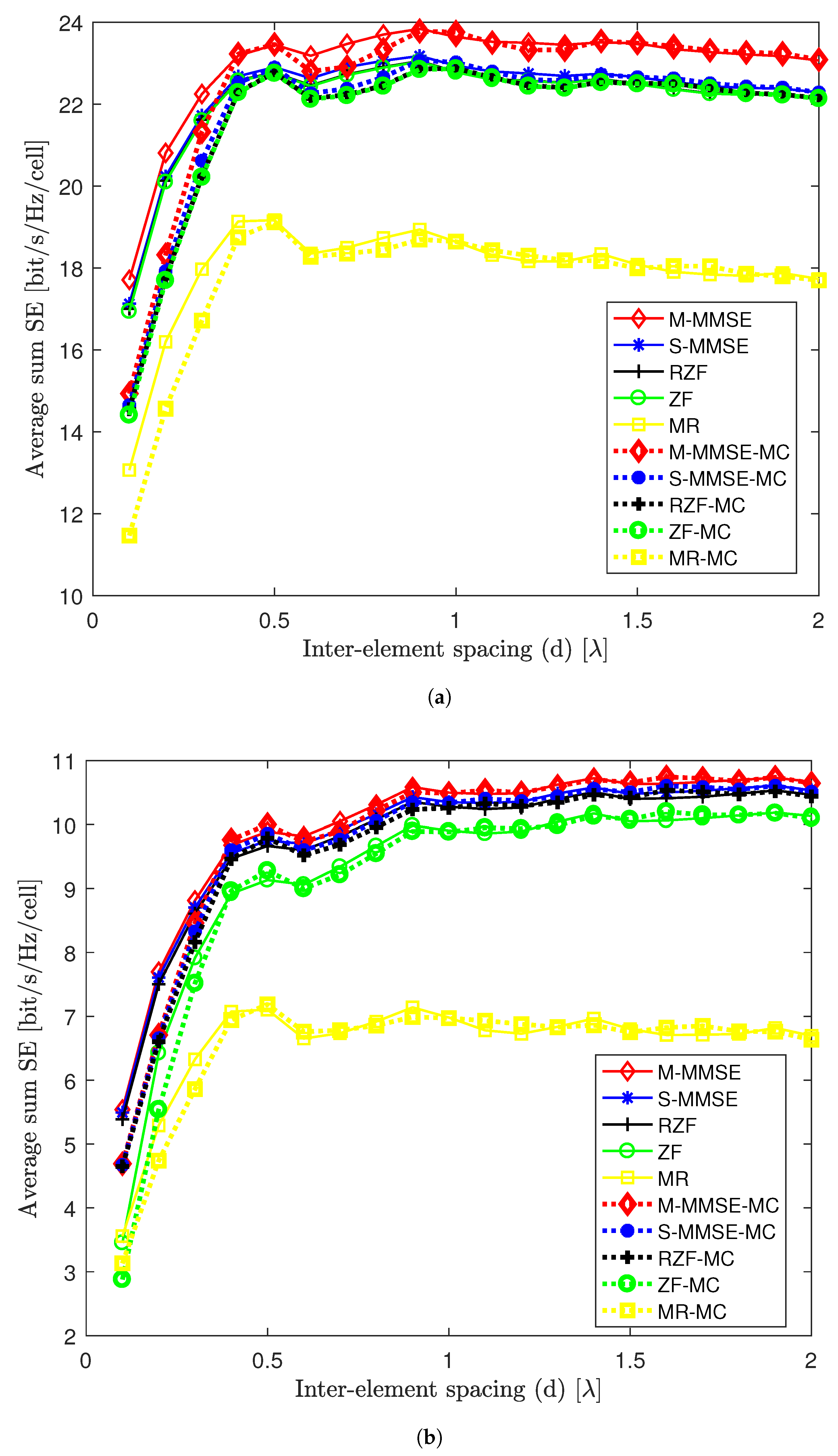
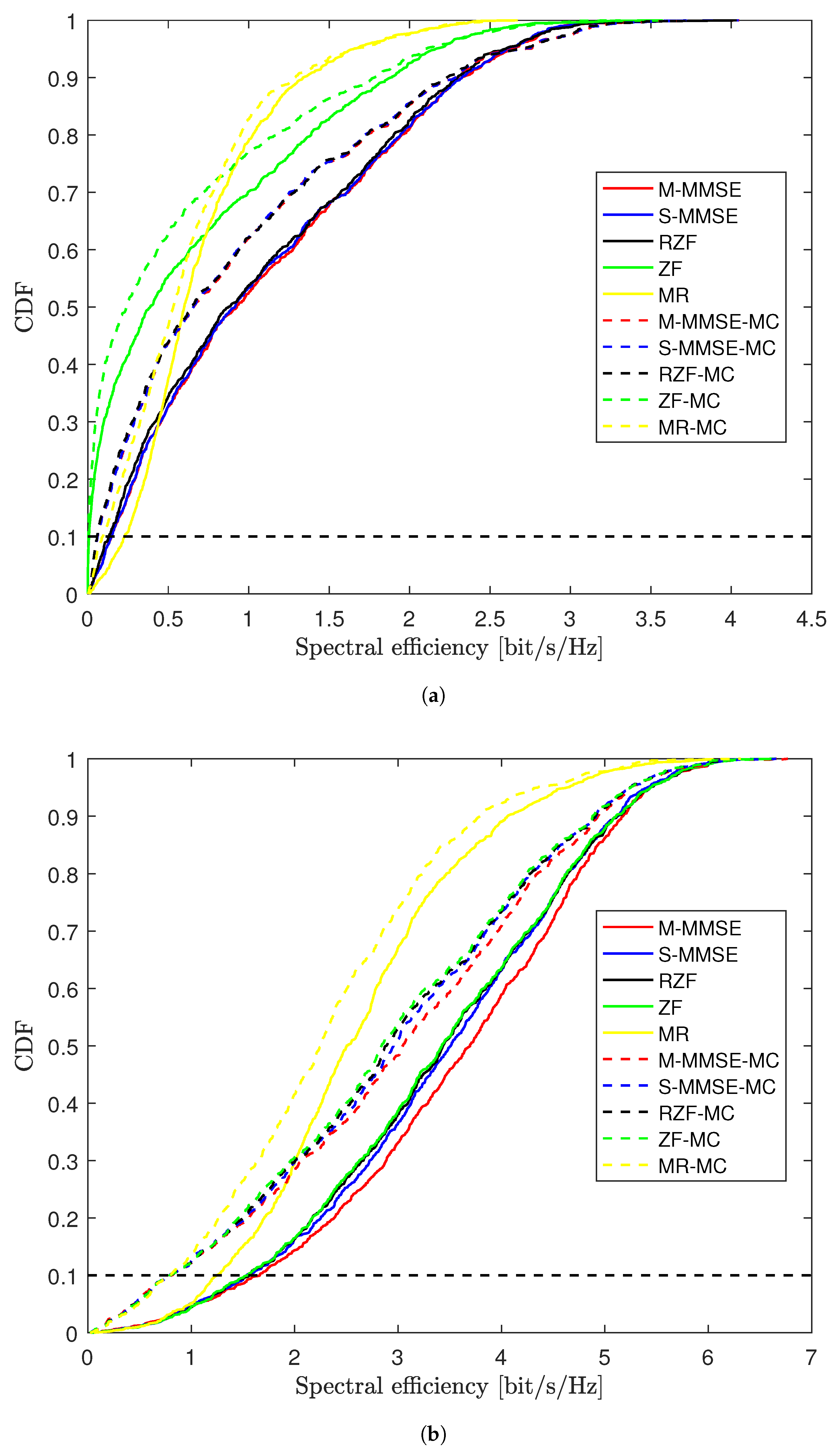
5. Performance Evaluation

In this section, we illustrate the simulation results to study the mutual coupling impact on the spectral efficiency of different precoding schemes, including MR, ZF, RZF, S-MMSE, and M-MMSE. To obtain a fair comparison, equal DL transmitted power is assumed to be allocated to different UEs. Additionally, the Gaussian local scattering model is used to construct the spatial correlation [25]. The BS is equipped with a large ULA antenna array, and it is assumed that every cell has the same number of UEs K m = K , m = 1 , 2 , , M . The value of the antenna impedance Z A in (8) is set to 73 + j 42.5 ohms. More detailed values of parameters are listed in Table 2.
Figure 2a shows the comparison of the spectral efficiency of different algorithms with or without mutual coupling, while varying the inter-element spacing d and fixing the number of antenna elements N at 200. We can find that the effect of mutual coupling on various schemes is similar, and the mutual coupling decreases the spectral efficiency under every scheme but does not change their orders of performance, with MR being the worst one no matter whether mutual coupling is considered or not. It is clear to see that every single curve of the spectral efficiency turns to rapidly rise with the increase of d when d is small and tends to be flat when d is larger than 0.5 λ . Without mutual coupling, the remarkable decrease of SE, as d goes to zero, mainly stems from the strong spatial correlation between antenna array elements. Meanwhile, when d is small, we can see a relatively obvious distinction under the same scheme between adding and not adding the mutual coupling effect, i.e., the smaller d is, the disparity is more evident. Taking M-MMSE scheme for example, when d = 0.1 λ , it yields about 17.2 bit/s/Hz/cell in average spectral efficiency without mutual coupling, and the number when we consider mutual coupling becomes 14.8 bit/s/Hz/cell, which brings a 14% decline. Furthermore, when 0.5 λ < d < 1 λ , there is a fluctuation under the impact of mutual coupling, which causes 0.8 bit/s/Hz/cell drop at most for four precoding schemes located above and is relatively moderate for MR. When d > 1 λ , the difference between considering and not considering mutual coupling under one scheme can be just negligible. All these conclusions are based on the premise that the number of antenna elements N is large.
Figure 2b compares the influences of mutual coupling under different schemes when the number of antenna elements N is fixed at 20, a relatively small number. We can see that the trend of all schemes remains the same as that depicted in Figure 2a, but the effect of the mutual coupling seems to be not that obvious, such as when N is large. When d is smaller than 0.5 λ , the number of spectral efficiencies under every scheme grows quickly, and we can easily distinguish whether the curve is with the mutual coupling or not. On a quantitative basis, when d = 0.1 λ , for the M-MMSE scheme, the spectral efficiency is 5.23 bit/s/Hz/cell, and after adding mutual coupling, the number is 4.60, decreasing by 12%, which is slightly less than that in Figure 2a. Note that when d = 0.1 λ , the ZF scheme with mutual coupling even achieves a worse performance than the MR scheme. When d is larger than 0.5 λ , the impact of mutual coupling on each scheme tends to recede and is significantly weak.
In Figure 3a, the mutual coupling impact on different schemes against various numbers of antenna elements is shown with inter-element spacing d = 0.1 λ . We can find that with the growth of the N, the average spectral efficiency of every scheme increases with one accord, and the growth rate turns to be gradually slower. It is clear that the schemes with mutual coupling are inferior to corresponding schemes ignoring mutual coupling. With the number of antenna elements N increasing from 20 to 200, the mutual coupling leads a negative effect on the growth rate of the average spectral efficiency, especially more obviously for the schemes that perform not so good in themselves For example, in the M-MMSE scheme, when we change N from 20 to 200, the spectral efficiency result increases from 5.23 to 17.2 bit/s/Hz/cell, and the growth rate is 228.74%. However, when mutual coupling is considered, the growth rate becomes 221.90% (from 4.60 to 14.8 bit/s/Hz/cell), which means the growth rate decreases by 7 percentage points or so due to the mutual coupling. As a contrast, in the MR scheme, performing worse than the M-MMSE scheme, the growth rate without mutual coupling is 279.76% (from 3.19 to 12.12 bit/s/Hz/cell), and the growth rate with mutual coupling is 266.46% (from 2.95 to 10.82 bit/s/Hz/cell), which leads a decrease of about 14 percentage points.
When we choose a larger inter-element spacing such as d = 2 λ , the relation of average spectral efficiency against the various number of antenna elements N is demonstrated in Figure 3b. It is evident that the performance of every scheme is so close that we can hardly tell them apart. Meanwhile, we can see no matter whether N is set at a smaller or larger number, the influence of mutual coupling on different schemes is just next to nothing, though it indeed exists under the premise of a large enough inter-element spacing d. In quantitative terms, when N = 200 , the mutual coupling only leads to a decrease of about 0.62%, from 23.68 to 23.53 bit/s/Hz/cell for the M-MMSE scheme, which has little effect on it. The findings indicate that the influence of mutual coupling is slight when d = 2 λ , regardless of how big N is.
Figure 4a,b exhibits the cumulative distribution function (CDF) of the SE of randomly located UEs to illustrate the comparison of different schemes with and without mutual coupling. For the case of that number of antenna elements N = 20 and the inter-element spacing d = 0.1 λ in Figure 4a, the vertical axis CDF = 0.1 line has already been labeled. This line refers to the 90% likely SE points. It is interesting that the MR scheme provides the highest SEs. Observing the whole curves of the CDF, it is clear that the MR scheme itself and MR scheme with mutual coupling curves cross the other curves, reflecting that no scheme can perform better than others for all UEs. M-MMSE, S-MMSE, and RZF schemes can exert better performance for UEs with good channel conditions.
While the parameters are set as the number of antenna elements N = 20 and the inter-element spacing d = 0.1 λ , Figure 4b is another try to compare the CDF curves of various schemes with mutual coupling or not. The general trend of these curves appears to have some difference when it is compared with Figure 4a. First, the M-MMSE scheme gives the highest SEs at the 90% likely SE points, and it also performs better than other schemes for all UEs almost as a whole. Second, from Figure 4a,b, every scheme gains in performance with varying degrees as the number of antennas increases, especially the ZF scheme. Third, when focusing on the 90% likely SE points, the negative effect of mutual coupling seems obvious: after adding the mutual coupling, every scheme except the MR scheme loses in SE apparently, even performing worse than the MR scheme without mutual coupling.
In general, antenna arrays cannot be infinitely large for practical reasons. To this end, we focus on the impact of mutual coupling on various algorithms under the premise that the antenna array size is fixed as a constant. Here, we consider the array size as N d , which is set as 40 λ , and the relation between average spectral efficiency against the number of antenna elements is illustrated in Figure 5. It can be seen that when N is less than 100, the performance of all schemes tends to increase with the growing of N, and the mutual coupling has little negative effect on each scheme among those. Particularly for the MR scheme, there is nearly no difference between taking and not taking mutual coupling into consideration when N < 80 . It is worth noting that when N is larger than 100, the impact of mutual coupling starts to appear. For the schemes without mutual coupling, when N continues to increase after N > 100 , the spectral efficiency accordingly enlarges as well, but for schemes with mutual coupling, the spectral efficiency stops rising when N is larger than 100, and some of them appear to remain unchanged or even descend. For instance, in the M-MMSE scheme, when N = 100 , we achieve its spectral efficiency with 18.68 bit/s/Hz/cell. As N continues rising, the scheme itself outperforms and up to N = 200 ofthe spectral efficiency increases to 20.50 bit/s/Hz/cell; that is a 9% promotion compared with the number when N = 100 . However, when mutual coupling is added, we obtain a poorer result of spectral efficiency, as 18.32 bit/s/Hz/cell when N = 200 , which means a 2% drop from 18.68 bit/s/Hz/cell. Hence, we can obtain a conclusion that when the antenna array size is determined, there is an optimal solution regarding the allocation of the number of antenna elements and the inter-element spacings, which can achieve the best performance of spectral efficiency when we consider the impact of mutual coupling. In the above scenario, the answer is when N = 100 (this also means d = 0.4 λ ), every scheme with mutual coupling can outperform and achieve its peak value in average sum spectral efficiency.
In Figure 6, under the premise that the antenna array size is fixed, the CDF of the SE of different schemes is compared. Two cases of parameters are considered here and put together in the figure: one is N = 20 , d = 2 λ depicted by the thin curves, and the other one is N = 200 , d = 0.2 λ depicted by the thick curves. For all schemes listed in the figure, the M-MMSE with N = 200 gives the best performance for every UE, and the MR gives the worst performance in contrast. From the figure, when N = 20 ( d = 2 λ ), the effect of mutual coupling cannot be distinguished, and the MR scheme has a lower upper limit value of SE, making its performance fall behind others. In the N = 200 ( d = 0.2 λ ) case, the mutual coupling brings the decrease of probability to achieve high SE values. As a result, when the antenna array size is fixed, precoding schemes with mutual coupling are more likely to suffer a great performance loss in a larger number of antenna elements N for every single UE.

6. Conclusions

In this paper, multi-cell multi-user massive MIMO communication systems with different precoding algorithms and mutual coupling effect have been investigated. Considering different precoding algorithms, the effect of the mutual coupling on the massive MIMO is first analyzed by the channel hardening method. Furthermore, it is interesting that the effect of mutual coupling on various schemes is similar, and the mutual coupling decreases the spectral efficiency under every scheme but does not change their orders of performance, with MR being the worst one no matter whether mutual coupling is considered or not. Our results provide meaningful guidelines for the massive MIMO system in practical scenarios. For future studies, we will try to investigate the energy efficiency of multi-cell multi-user massive MIMO communication systems. Additionally, we can take other practical factors into consideration, such as hardware impairments of the antenna array, which might result in imperfect channel reciprocity, or channel aging when we consider the mobility of UEs to improve the model for evaluating the mutual coupling effects.

Author Contributions

Conceptualization, Y.L. and B.A.; methodology, Y.L.; software, Y.L.; validation, J.Z.; formal analysis, Y.L.; investigation, J.Z.; resources, B.A.; data curation, Y.L.; writing—original draft preparation, Y.L.; writing—review and editing, J.Z.; visualization, J.Z.; supervision, B.A.; project administration, B.A.; funding acquisition, B.A. All authors have read and agreed to the published version of the manuscript.

Funding

This work was supported in part by the State Key Laboratory of Rail Traffic Control and Safety (Contract No. RCS2022ZQ005).

Data Availability Statement

Not applicable.

Conflicts of Interest

The authors declare no conflict of interest. The funders had no role in the design of the study; in the collection, analyses, or interpretation of data; in the writing of the manuscript; or in the decision to publish the results.

References

  1. Larsson, E.G.; Edfors, O.; Tufvesson, F.; Marzetta, T.L. Massive MIMO for next generation wireless systems. IEEE Commun. Mag. 2014, 52, 186–195. [Google Scholar] [CrossRef] [Green Version]
  2. Zhang, J.; Björnson, E.; Matthaiou, M.; Ng, D.W.K.; Yang, H.; Love, D.J. Prospective multiple antenna technologies for beyond 5G. IEEE J. Sel. Areas Commun. 2020, 38, 1637–1660. [Google Scholar] [CrossRef]
  3. Shao, Z.; Yan, W.; Yuan, X. Markovian Cascaded Channel Estimation for RIS Aided Massive MIMO Using 1-Bit ADCs and Oversampling. ZTE Commun. 2022, 20, 48–56. [Google Scholar]
  4. Zhang, J.; Dai, L.; Li, X.; Liu, Y.; Hanzo, L. On low-resolution ADCs in practical 5G millimeter-wave massive MIMO systems. IEEE Commun. Mag. 2018, 56, 205–211. [Google Scholar] [CrossRef] [Green Version]
  5. Manteuffel, D.; Lin, F.H.; Li, T.; Peitzmeier, N.; Chen, Z.N. Characteristic Mode-Inspired Advanced Multiple Antennas: Intuitive insight into element-, interelement-, and array levels of compact large arrays and metantennas. IEEE Antennas Propag. Mag. 2022, 64, 49–57. [Google Scholar] [CrossRef]
  6. Chen, X.; Zhang, S.; Li, Q. A review of mutual coupling in MIMO systems. IEEE Access 2018, 6, 24706–24719. [Google Scholar] [CrossRef]
  7. Chang, M.; Han, J.; Ma, X.; Xue, H.; WU, X.; Li, L.; Cui, T. Programmable Metasurface for Simultaneously Wireless Information and Power Transfer System. ZTE Commun. 2022, 20, 48–62. [Google Scholar]
  8. Hassan, S.u.; Mir, T.; Alamri, S.; Khan, N.A.; Mir, U. Machine Learning-Inspired Hybrid Precoding for HAP Massive MIMO Systems with Limited RF Chains. Electronics 2023, 12, 893. [Google Scholar] [CrossRef]
  9. Kassam, J.; Castanheira, D.; Silva, A.; Dinis, R.; Gameiro, A. A Review on Cell-Free Massive MIMO Systems. Electronics 2023, 12, 1001. [Google Scholar] [CrossRef]
  10. Clerckx, B.; Craeye, C.; Vanhoenacker-Janvier, D.; Oestges, C. Impact of Antenna Coupling on 2 × 2 MIMO Communications. IEEE Trans. Veh. Technol. 2007, 56, 1009–1018. [Google Scholar] [CrossRef]
  11. Masouros, C.; Sellathurai, M.; Ratnarajah, T. Large-Scale MIMO Transmitters in Fixed Physical Spaces: The Effect of Transmit Correlation and Mutual Coupling. IEEE Trans. Commun. 2013, 61, 2794–2804. [Google Scholar] [CrossRef]
  12. Neil, C.T.; Garcia-Rodriguez, A.; Smith, P.J.; Dmochowski, P.A.; Masouros, C.; Shafi, M. On the Performance of Spatially Correlated Large Antenna Arrays for Millimeter-Wave Frequencies. IEEE Trans. Antennas Propag. 2018, 66, 132–148. [Google Scholar] [CrossRef]
  13. Biswas, S.; Masouros, C.; Ratnarajah, T. Performance Analysis of Large Multiuser MIMO Systems With Space-Constrained 2-D Antenna Arrays. IEEE Trans. Wirel. Commun. 2016, 15, 3492–3505. [Google Scholar] [CrossRef] [Green Version]
  14. Gustafsson, M.; Aulin, J.; Högberg, M.; Alm, M.; Sihlbom, B. Impact of mutual coupling on capacity in large MIMO antenna arrays. In Proceedings of the 8th European Conference on Antennas and Propagation (EuCAP 2014), The Hague, The Netherlands, 6–11 April 2014; pp. 2723–2727. [Google Scholar] [CrossRef]
  15. Pfeiffer, C.; Dagefu, F.; Tomasic, B.; Twigg, J.N.; Wu, B.I. Virtual Impedance Method for Mutual Coupling Compensation. IEEE Trans. Antennas Propag. 2021, 69, 4569–4579. [Google Scholar] [CrossRef]
  16. Xiao, Y.; Wang, Y. Deep Learning-Based Mutual Coupling Modeling and Baseband Decoupling Algorithm for MIMO Systems. IEEE Commun. Lett. 2020, 24, 1986–1990. [Google Scholar] [CrossRef]
  17. Zhang, J.; Zhang, J.; Björnson, E.; Ai, B. Local partial zero-forcing combining for cell-free massive MIMO systems. IEEE Trans. Commun. 2021, 69, 8459–8473. [Google Scholar] [CrossRef]
  18. Tian, Y.; Wang, R.; Chen, H.; Qin, Y.; Jin, M. Real-Valued DOA Estimation Utilizing Enhanced Covariance Matrix With Unknown Mutual Coupling. IEEE Commun. Lett. 2022, 26, 912–916. [Google Scholar] [CrossRef]
  19. Zhang, S.; Chen, X.; Pedersen, G.F. Mutual Coupling Suppression With Decoupling Ground for Massive MIMO Antenna Arrays. IEEE Trans. Veh. Technol. 2019, 68, 7273–7282. [Google Scholar] [CrossRef]
  20. Chen, K.H.; Kiang, J.F. Effect of mutual coupling on the channel capacity of MIMO systems. IEEE Trans. Veh. Technol. 2015, 65, 398–403. [Google Scholar] [CrossRef]
  21. Wei, H.; Wang, D.; Zhu, H.; Wang, J.; Sun, S.; You, X. Mutual Coupling Calibration for Multiuser Massive MIMO Systems. IEEE Trans. Wirel. Commun. 2016, 15, 606–619. [Google Scholar] [CrossRef]
  22. Ge, X.; Zi, R.; Wang, H.; Zhang, J.; Jo, M. Multi-User Massive MIMO Communication Systems Based on Irregular Antenna Arrays. IEEE Trans. Wirel. Commun. 2016, 15, 5287–5301. [Google Scholar] [CrossRef] [Green Version]
  23. Amani, N.; Wymeersch, H.; Johannsen, U.; Smolders, A.B.; Ivashina, M.V.; Maaskant, R. Multi-Panel Sparse Base Station Design With Physical Antenna Effects in Massive MU-MIMO. IEEE Trans. Veh. Technol. 2020, 69, 6500–6510. [Google Scholar] [CrossRef] [Green Version]
  24. Raeesi, O.; Gokceoglu, A.; Zou, Y.; Björnson, E.; Valkama, M. Performance Analysis of Multi-User Massive MIMO Downlink Under Channel Non-Reciprocity and Imperfect CSI. IEEE Trans. Commun. 2018, 66, 2456–2471. [Google Scholar] [CrossRef] [Green Version]
  25. Bjornson, E.; Hoydis, J.; Sanguinetti, L. Massive MIMO Networks Spectral, Energy, and Hardware Efficiency. In Foundations and Trends® in Signal Processing; Weizmann Institute: Rehovot, Israel, 2017; Volume 11, pp. 154–655. [Google Scholar]
  26. Balanis, C.A. Antenna Theory: Analysis and Design, 4th ed.; Wiley-Blackwell: Hoboken, NJ, USA, 2016. [Google Scholar]
  27. Ngo, H.Q.; Larsson, E.G. No Downlink Pilots Are Needed in TDD Massive MIMO. IEEE Trans. Wirel. Commun. 2017, 16, 2921–2935. [Google Scholar] [CrossRef] [Green Version]
  28. Hoydis, J.; ten Brink, S.; Debbah, M. Massive MIMO in the UL/DL of Cellular Networks: How Many Antennas Do We Need? IEEE J. Sel. Areas Commun. 2013, 31, 160–171. [Google Scholar] [CrossRef] [Green Version]
  29. Jose, J.; Ashikhmin, A.; Marzetta, T.L.; Vishwanath, S. Pilot Contamination and Precoding in Multi-Cell TDD Systems. IEEE Trans. Wirel. Commun. 2011, 10, 2640–2651. [Google Scholar] [CrossRef] [Green Version]
Figure 1. Downlink multi-cell massive MIMO systems.
Electronics 12 01364 g001
Figure 2. Spectral efficiency comparison of different algorithms with and without mutual coupling vs. inter-element spacing d when the number of antenna elements (a) N = 200 , (b) N = 20 .
Electronics 12 01364 g002
Figure 3. Spectral efficiency comparison of different algorithms with and without mutual coupling vs. the number of antenna elements N when inter-element spacing (a) d = 0.1 λ (b) d = 2 λ .
Electronics 12 01364 g003
Figure 4. CDF of the spectral efficiency with and without mutual coupling when inter-element spacing d = 0.1 λ and the number of antenna elements (a) N = 20 , (b) N = 200 .
Electronics 12 01364 g004
Figure 5. Spectral efficiency comparison of different algorithms with and without mutual coupling vs. inter-element spacing d when the array size is fixed.
Electronics 12 01364 g005
Figure 6. CDF of the spectral efficiency with and without mutual coupling when the antenna array size is fixed.
Electronics 12 01364 g006
Table 1. Comparison with previous representative research papers.
MC Effect Ref.MC Effect Modeling MethodPrecoding SchemesClosed-Form ExpressionsMulti-UserMulti-Cell
[12]Impedance matrix-basedHBFCoveredSingle userSingle cell
[13]Impedance matrix-basedZF and MRTCoveredMulti-userSingle cell
[14]S-parameter-basedNot coveredNot coveredSingle userSingle cell
[23]Simulation plus impedance matrix-basedZFNot coveredMulti-userSingle cell
[24]Statistical distribution-basedZF and MRTCoveredMulti-userSingle cell
[16]Deep learning-basedHBFNot coveredSingle userSingle cell
Our workImpedance matrix-basedMRT, ZF, RZF, S-MMSE, M-MMSECoveredMulti-userMulti-cell
Table 2. Parameter settings.
SymbolsParametersValues
f c Carrier frequency2 GHz
BSystem Bandwidth200 MHz
ASDangular standard deviation10
Mthe number of cells4
Kthe number of UEs5
P t Transmit power per UE20 dBm
N 0 Background noise density−174 dBm/Hz
Disclaimer/Publisher’s Note: The statements, opinions and data contained in all publications are solely those of the individual author(s) and contributor(s) and not of MDPI and/or the editor(s). MDPI and/or the editor(s) disclaim responsibility for any injury to people or property resulting from any ideas, methods, instructions or products referred to in the content.

