
Non-Contact Measurement Method of Phase Current Based on Magnetic Field Decoupling Calculation for Three-Phase Four-Core Cable
Abstract
:1. Introduction
2. Measurement Structure and Principle
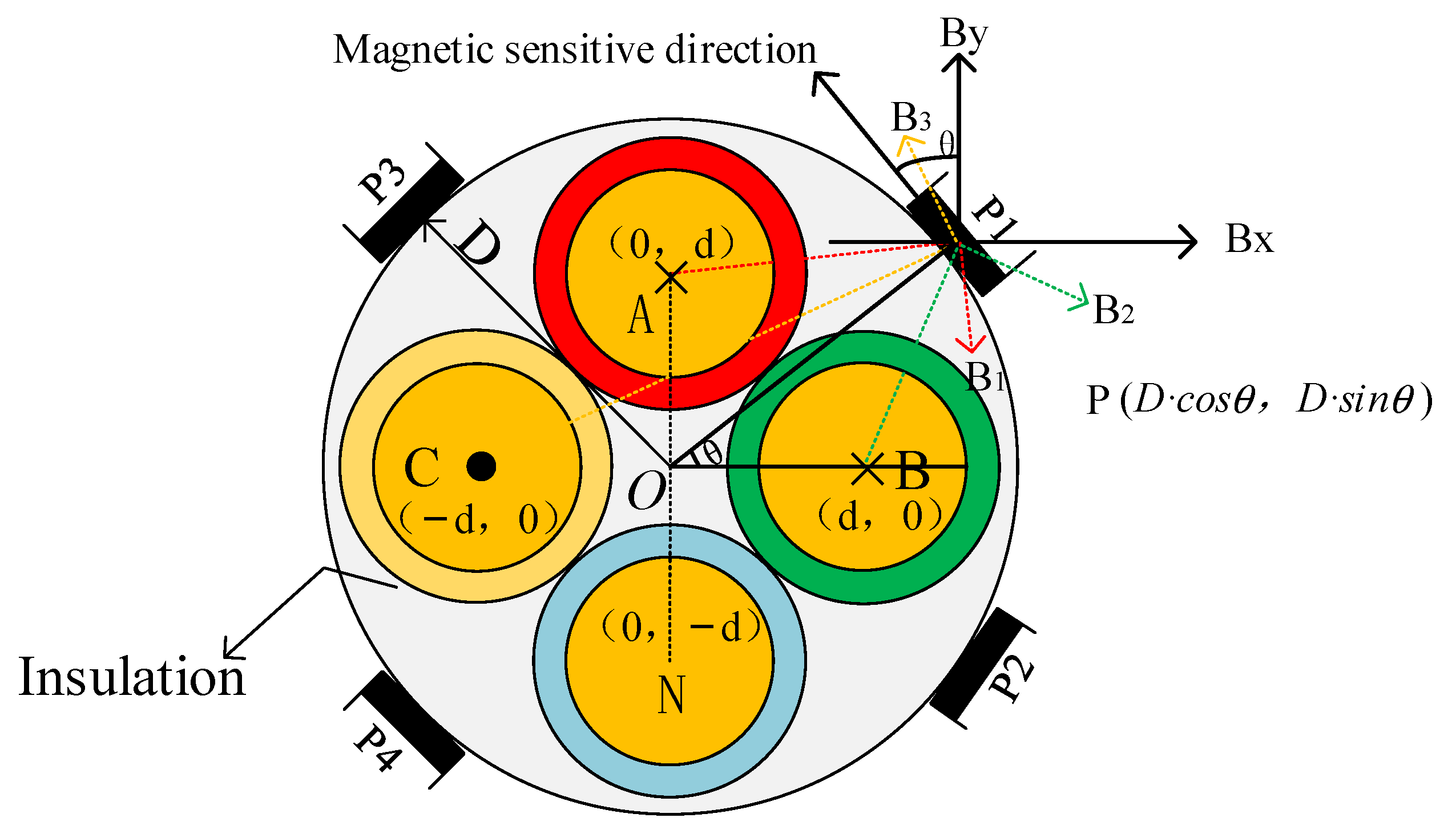
2.1. Determination of Measurement Model
2.2. Principle of Magnetic Field Coupling Measurement and Determination of Decoupling Coefficient
3. Current Reconstruction Technology
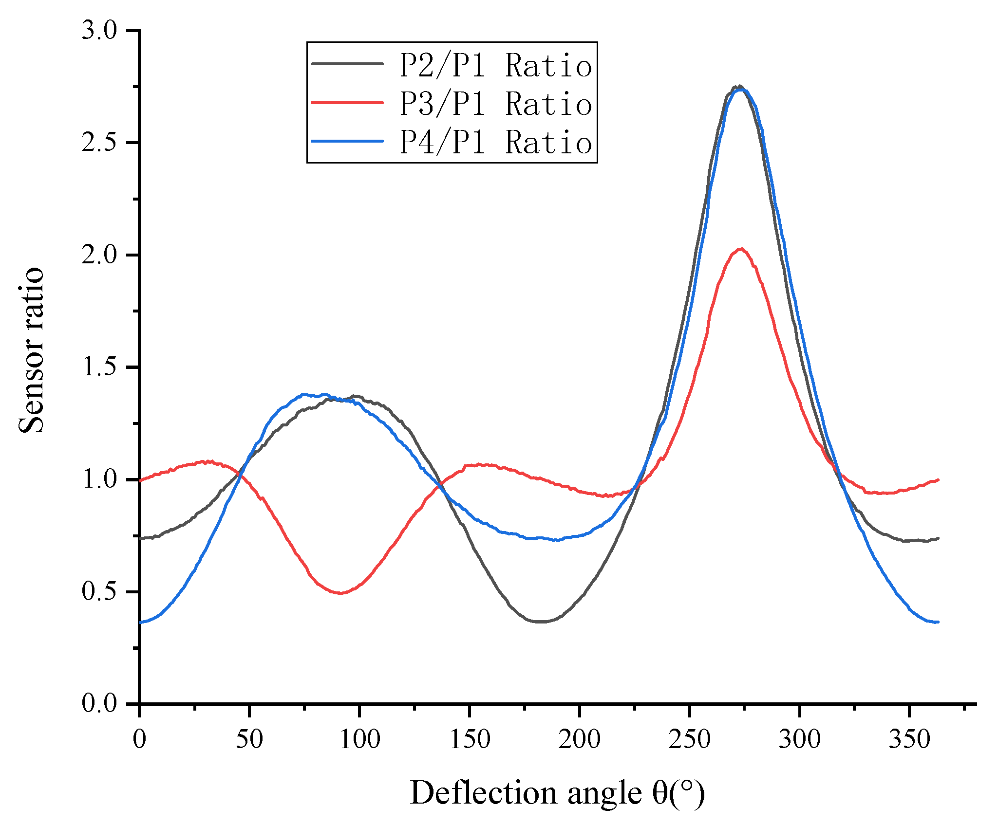
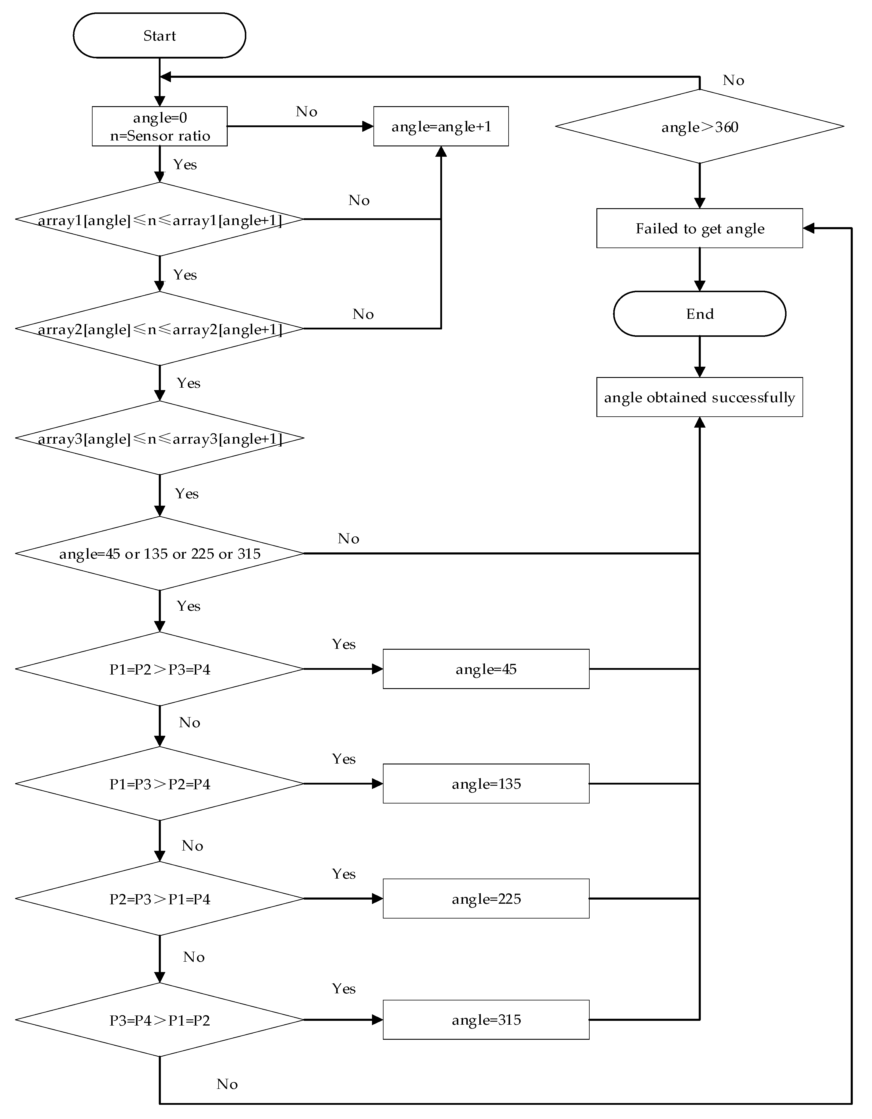
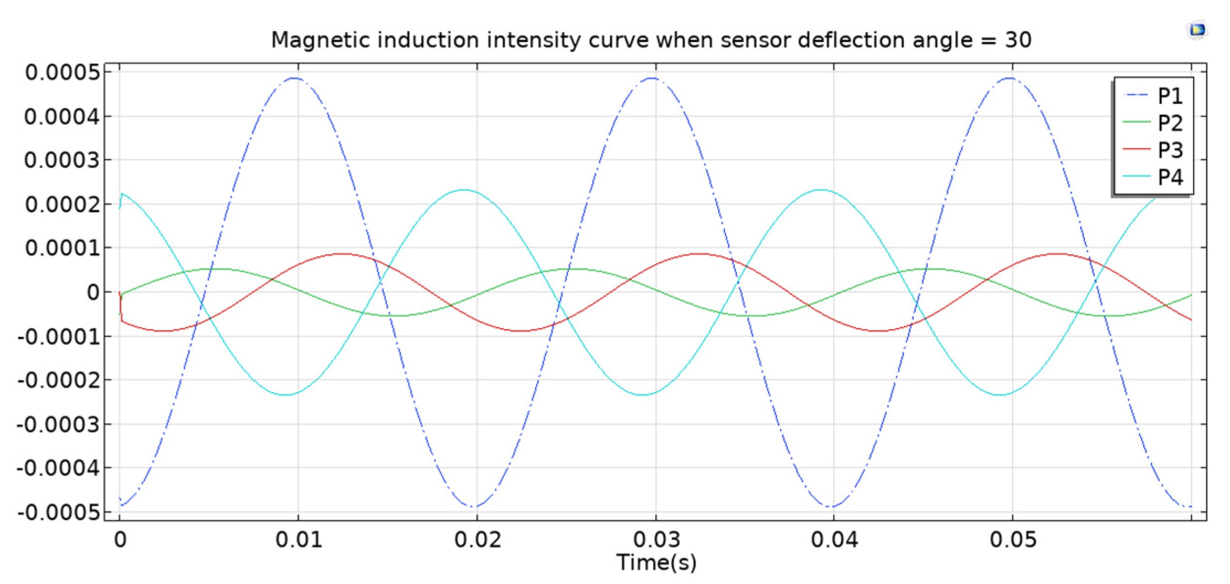
3.1. Determination of Deflection Angle
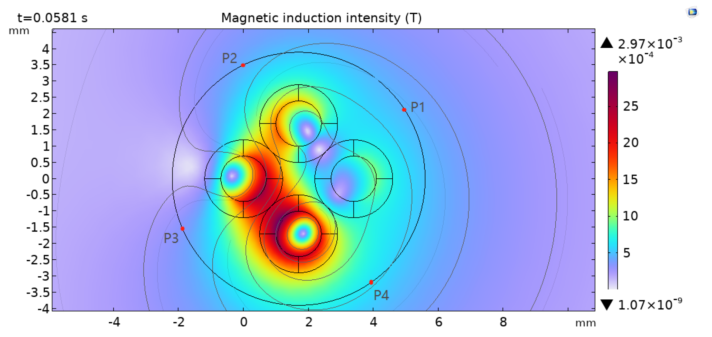
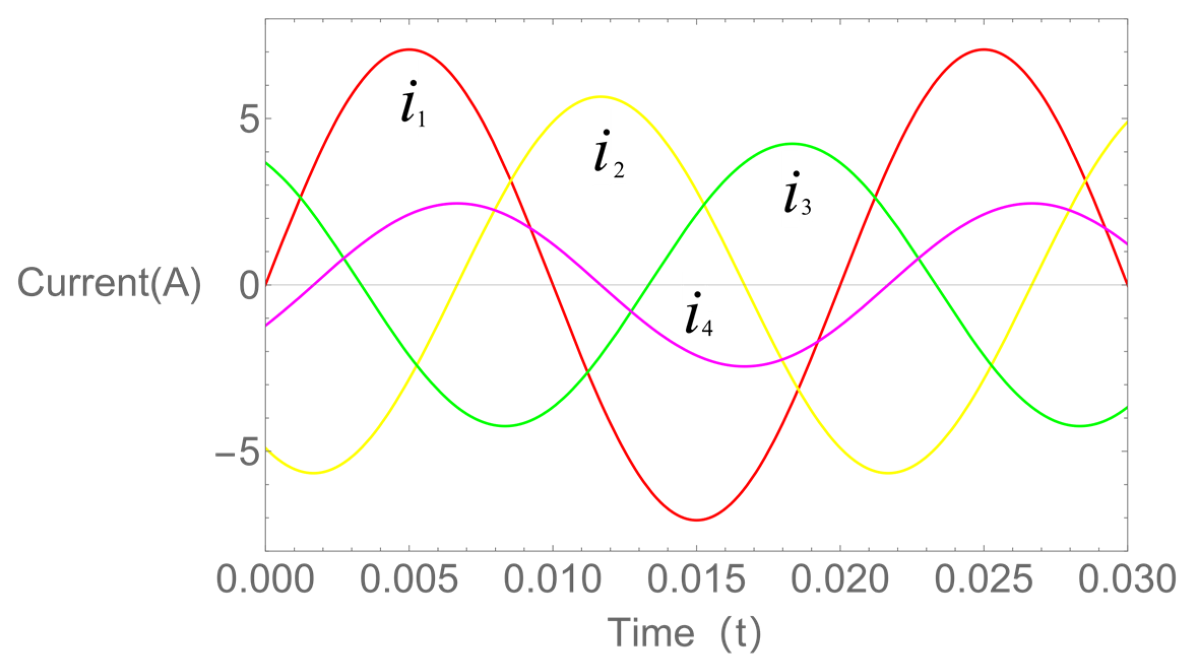
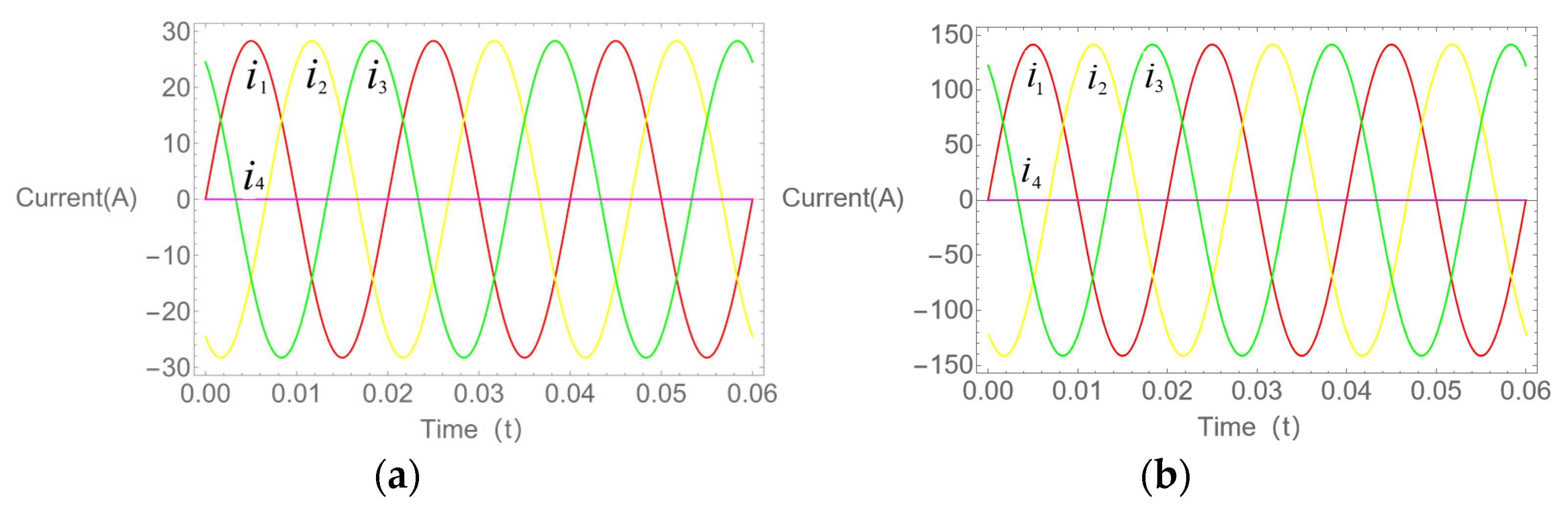
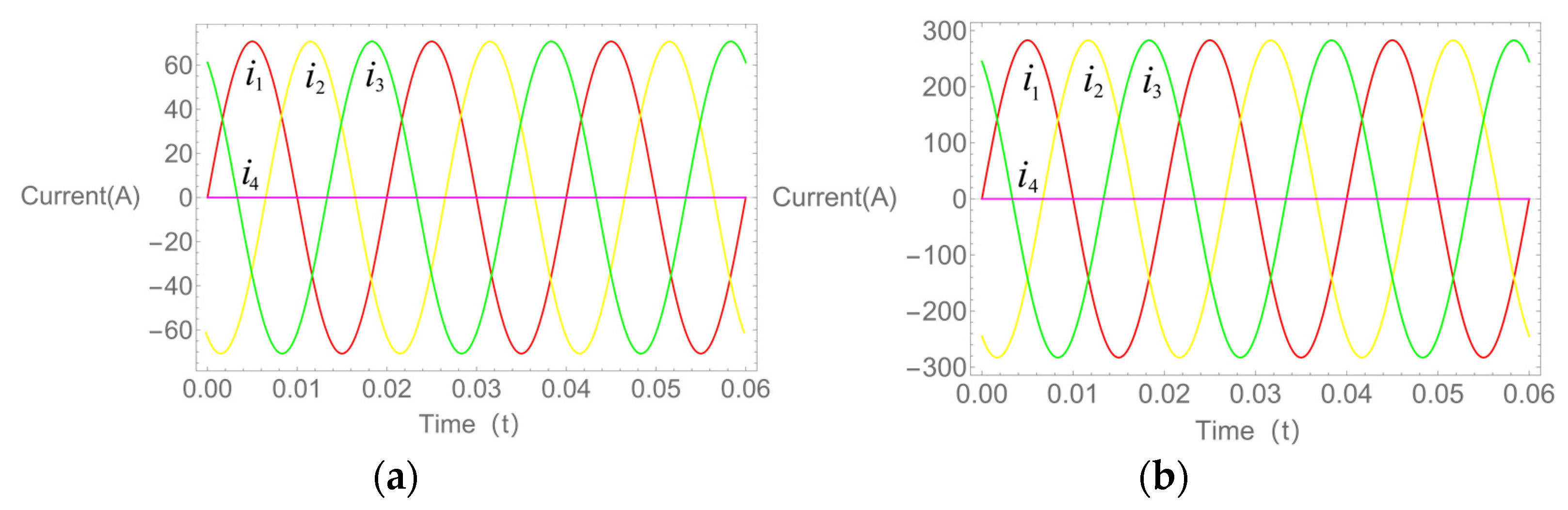
3.2. Three-Phase Current Simulation and Reconstruction
3.3. Evaluation of Reconstruction Current Accuracy
3.4. Reduction of Cable Current with Different Section Sizes
4. Design of Magnetic Array Current Sensor
4.1. Measuring Principle of Fluxgate Sensor
4.2. Design of Peripheral Parameters of Magnetic Array Sensor
4.3. Matrix Relationship between Sensor Output Voltage and Three-Phase Current
5. Experimental Verification
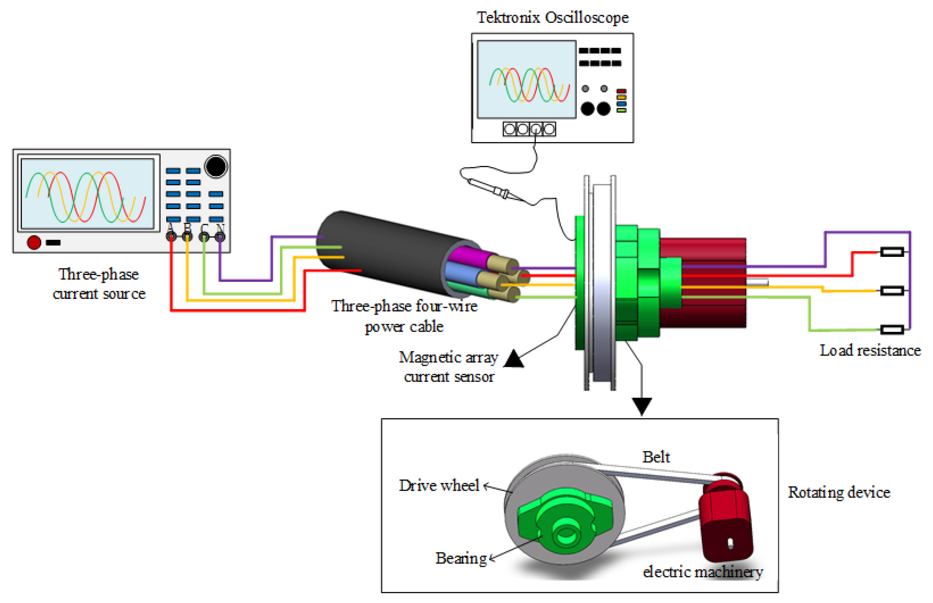
5.1. Establishment of Experimental Platform
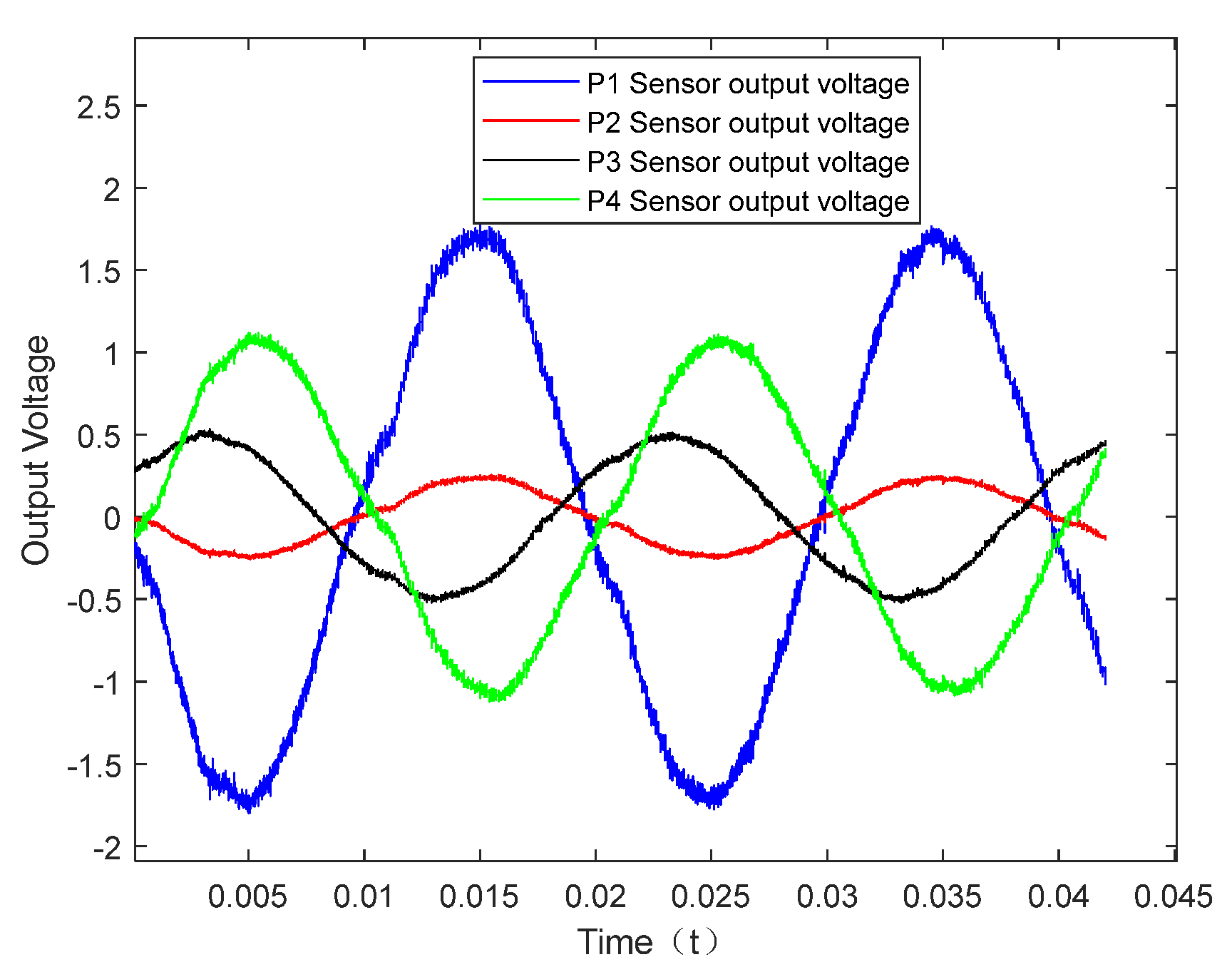
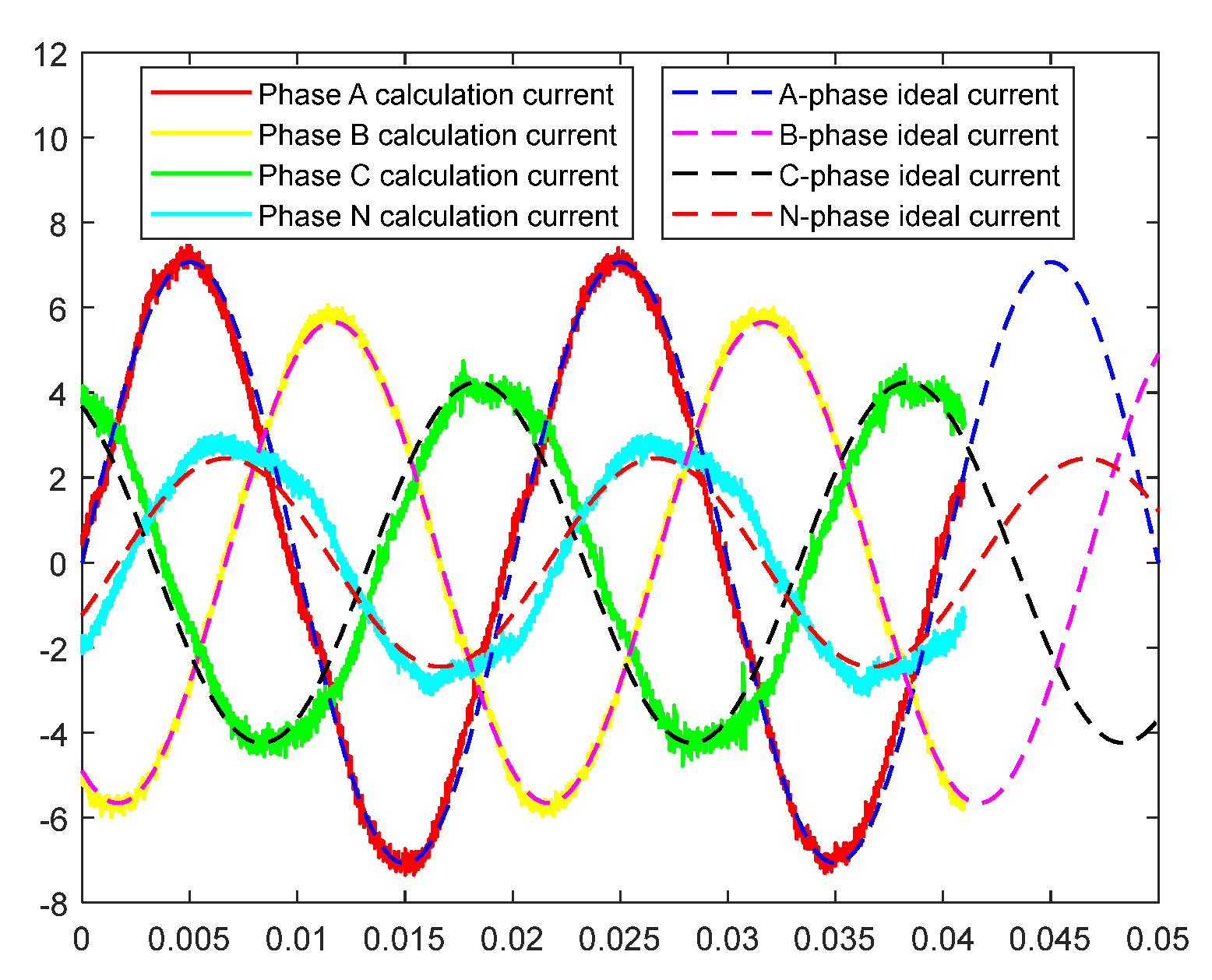
5.2. Analysis and Discussion of Experimental Results
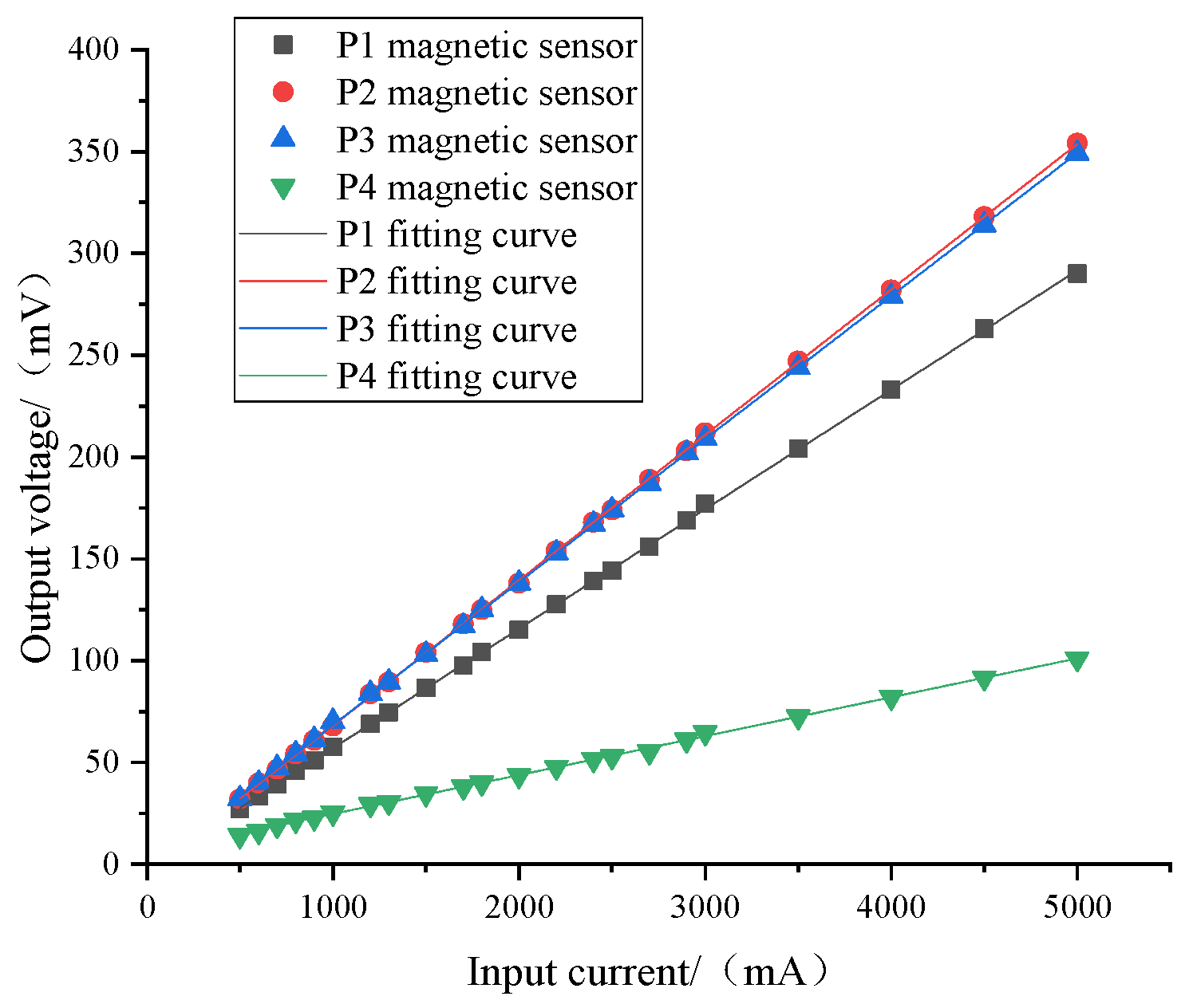
5.3. Linear Error and Sensitivity of Sensor
6. Conclusions
Author Contributions
Funding
Acknowledgments
Conflicts of Interest
Appendix A
References
- Yang, Q.; Sun, S.; Sima, W.; He, Y.; Luo, M. Research progress of advanced voltage and current sensing methods for smart grid. High Volt. Eng. 2019, 45, 349–367. [Google Scholar]
- Wang, Y.; Xie, J.; Lu, F.; Li, M.; Yan, C.; Bi, J.; Yuan, S. Overvoltage monitoring method based on composite integral Rogowski coil. Power Syst. Technol. 2015, 39, 1450–1455. [Google Scholar]
- Donnal, J.S. Home NILM: A Comprehensive Energy Monitoring Toolkit; Massachusetts Institute of Technology: Cambridge, MA, USA, 2013. [Google Scholar]
- Xiao, D.; Ma, Q.; Xie, Y.; Zheng, Q.; Zhang, Z. A Power-Frequency Electric Field Sensor for Portable Measurement. Sensor 2018, 18, 1053. [Google Scholar] [CrossRef] [PubMed] [Green Version]
- Casallas, A. Contactless Voltage and Current Estimation Using Signal Processing and Machine Learning; Massachusetts Institute of Technology: Cambridge, MA, USA, 2019. [Google Scholar]
- Guo, W.; Zhou, S.; Wang, L.; Pei, H.; Cheng, Z.; Li, H. Design and application of power cable condition online monitoring system. High Volt. Eng. 2019, 45, 3459–3466. [Google Scholar]
- Ma, G.; Wang, S.; Qin, W.; Zhang, B.; Zhang, J.; Chen, C. Research and Prospect of Optical Fiber Sensing of Transmission Line Operation Status. High Volt. Eng. 2022, 48, 3032–3047. [Google Scholar]
- Sun, T. Three-core cable self-energy extraction method and its application in thermal state monitoring. High Volt. Appar. 2019, 55, 215–220. [Google Scholar]
- Sun, X.; Poon, C.K.; Chan, G.; Sum, C.L.; Lee, W.K.; Jiang, L.; Pong, P.W. Operation-State Monitoring and Energization-StatusIdentification for Underground Power Cables by Magnetic Field Sensing. IEEE Sens. J. 2013, 13, 4527–4533. [Google Scholar] [CrossRef] [Green Version]
- Donnal, J.S.; Leeb, S.B. Noncontact Power Meter. IEEE Sens. J. 2015, 15, 1161–1169. [Google Scholar] [CrossRef]
- Geng, J.; Xin, Z.; Shi, Y.; Liu, X. Non-Contact Electric Field Coupled Voltage Sensor for SiC MOSFET Switching Voltage Measurement. Proc. CSEE. 2022. Available online: https://kns.cnki.net/kcms/detail/11.2107.TM.20220309.1210.004.html (accessed on 14 March 2023).
- Zhang, S.; Chen, Z.; Ma, C.; Chen, Q.; Liu, T.; Tan, Y. Three-Phase Cable Voltage Non-Contact Measurement Method Based on Electric Field Inverse Calculation. Electr. Meas. Instrum. 2022. Available online: https://kns.cnki.net/kcms/detail/23.1202.th.20220817.1505.010.html (accessed on 14 March 2023).
- Donnal, J.S.; Lindahl, P.; Lawrence, D.; Zachar, R.; Leeb, S. Untangling Non-Contact Power Monitoring Puzzles. IEEE Sens. J. 2017, 17, 3542–3550. [Google Scholar] [CrossRef]
- Ibrahim, M.E.; Abd-Elhady, A.M. A Proposed Non-Invasive Rogowski Coil Design for Measuring 3-Phase Currents Through a 3-Core Cable. IEEE Sens. J. 2020, 21, 1. [Google Scholar] [CrossRef]
- Selva, K.T.; Forsberg, O.A.; Merkoulova, D.; Ghasemifard, F.; Taylor, N.; Norgren, M. Non-Contact Current Measurement in Power Transmission Lines. Procedia Technol. 2015, 21, 498–506. [Google Scholar] [CrossRef]
- Hou, Y. Research on Piezoelectric Beam-Type Current Sensor for Three-Phase Four-Wire Conductor; Jilin University: Changchun, China, 2019. [Google Scholar]
- Gong, S. Research on Current Fault Detection Mechanism of Three-Phase Five-Wire Cable; Jilin University: Changchun, China, 2022. [Google Scholar]
- Zhao, Z. Research on High Universality Passive Non-Intrusive Current Sensor; Jilin University: Changchun, China, 2021. [Google Scholar]
- Liu, H. Research on Passive Passive Non-Contact Current Sensing Mechanism and Measurement Method; Jilin University: Changchun, China, 2018. [Google Scholar]
- Xiao, D.; Jiang, K.; Liu, H.; Zhou, Q.; Li, S. Inversion and inverse method from power frequency magnetic field data to three-phase current of overhead transmission lines. Proc. CSEE 2016, 36, 1438–1444. [Google Scholar]
- Lawrence, D.; Donnal, J.S.; Leeb, S. Current and Voltage Reconstruction From Non-Contact Field Measurements. IEEE Sens. J. 2016, 16, 6095–6103. [Google Scholar] [CrossRef]
- Bai, X. Research on Three-Phase Unbalanced Current Detection Method of Non-Contact Underground Cable Based on Magnetic Field Measurement; Three Gorges University: Yichang, China, 2017. [Google Scholar]
- Song, X.; Ren, W.; Suo, Y.; Jia, L.; Long, T. Calibration method of three-axis magnetic field decoupling magnetic compensation for single-beam SERF magnetometer. Chin. J. Sci. Instrum. 2022, 43, 55–62. [Google Scholar]
- Yao, J.; Wang, J.; Wang, J.; Geng, Y. Theoretical study on interference elimination when magnetic sensor array is used to measure current. Proc. CSEE 2004, 12, 164–168. [Google Scholar]
- Li, C.; Xu, Q. Coupling analysis of magnetic field and temperature field of magnetic-collecting optical current sensor. Power Syst. Technol. 2014, 38, 9. [Google Scholar]
- Li, T. Technical Research on Residual Current Detection System under Complex Waveform Conditions; Kunming University of Science and Technology: Kunming, China, 2021. [Google Scholar]
- Cheng, S.; Jiang, X.; Xia, L.; Wan, S. Three-phase current measurement of single current sensor based on TMS320F240. Instrum. Technol. Sens. 2002, 5, 38–40. [Google Scholar] [CrossRef]


| Array1 (P2/P1) | Array2 (P3/P1) | Array3 (P4/P1) | |
|---|---|---|---|
| 0 | 0.734912 | 0.993191 | 0.363180 |
| 1 | 0.739019 | 0.997070 | 0.364397 |
| 2 | 0.737446 | 1.001517 | 0.366266 |
| … | … | … | … |
| 357 | 0.734047 | 0.992519 | 0.367433 |
| 358 | 0.731474 | 0.991843 | 0.364359 |
| 359 | 0.732534 | 0.993064 | 0.363779 |
| Phase Sequence | a | b | ||
|---|---|---|---|---|
| A | 7.09 | 0.02 | 7.10 | 0.5 |
| B | −2.81 | −4.90 | 5.64 | −121.8 |
| C | −2.11 | 3.67 | 4.23 | 122.5 |
| N | 2.13 | −1.22 | 2.45 | −28.8 |
| Phase Sequence | Valid Value | Amplitude Error (%) | Phase Angle Error (°) |
|---|---|---|---|
| A | 5.0619 | 1.44 | −1.8 |
| B | 4.0825 | 2.06 | 1.98 |
| C | 3.0845 | 2.81 | 2.78 |
| N | 2.3867 | 2.56 | 1.3 |
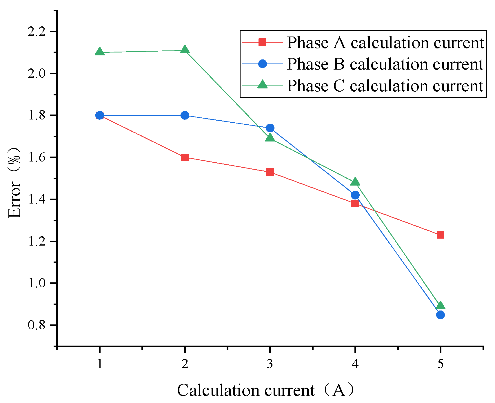
| Phase Sequence/Current | 1 A | 2 A | 3 A | 4 A |
|---|---|---|---|---|
| Error (%) | ||||
| A | 1.8 | 1.6 | 1.53 | 1.38 |
| B | 1.8 | 1.8 | 1.74 | 1.42 |
| C | 2.1 | 2.1 | 1.69 | 1.48 |
Disclaimer/Publisher’s Note: The statements, opinions and data contained in all publications are solely those of the individual author(s) and contributor(s) and not of MDPI and/or the editor(s). MDPI and/or the editor(s) disclaim responsibility for any injury to people or property resulting from any ideas, methods, instructions or products referred to in the content. |
© 2023 by the authors. Licensee MDPI, Basel, Switzerland. This article is an open access article distributed under the terms and conditions of the Creative Commons Attribution (CC BY) license (https://creativecommons.org/licenses/by/4.0/).
Share and Cite
Suo, C.; Cheng, K.; Wang, L.; Zhang, W.; Liu, X.; Zhu, J. Non-Contact Measurement Method of Phase Current Based on Magnetic Field Decoupling Calculation for Three-Phase Four-Core Cable. Electronics 2023, 12, 1443. https://doi.org/10.3390/electronics12061443
Suo C, Cheng K, Wang L, Zhang W, Liu X, Zhu J. Non-Contact Measurement Method of Phase Current Based on Magnetic Field Decoupling Calculation for Three-Phase Four-Core Cable. Electronics. 2023; 12(6):1443. https://doi.org/10.3390/electronics12061443
Chicago/Turabian StyleSuo, Chunguang, Kang Cheng, Lifeng Wang, Wenbin Zhang, Xi Liu, and Junyu Zhu. 2023. "Non-Contact Measurement Method of Phase Current Based on Magnetic Field Decoupling Calculation for Three-Phase Four-Core Cable" Electronics 12, no. 6: 1443. https://doi.org/10.3390/electronics12061443