Ground-Based MIMO-SAR Fast Imaging Algorithm Based on Geometric Transformation

Abstract

Ground-based multiple-input multiple-output synthetic aperture radar (MIMO-SAR) is a new type of deformation monitoring sensor that has the advantages of no mechanical motion and fast echo acquisition. Ground-based MIMO-SAR can significantly improve the data rate of deformation monitoring. In this paper, a fast imaging algorithm tailored for ground-based MIMO-SAR data is proposed, which can be applied in both far-field and near-field scenarios. First, the phase center approximation error of the non-collinear array in the near field is analyzed. Then, a fast imaging algorithm based on geometric transformation for the coherent synthesis of subimages is put forward. The algorithm uses the geometric transformation to convert the subaperture imaging results into the full aperture coordinate system, which avoids the point-by-point interpolation calculation and further reduces the computational cost of the subimage coherent synthesis algorithm. Simulations and experiments show that the algorithm can achieve high-precision focusing imaging, and its operation efficiency is significantly improved compared with the algorithm based on interpolation.

1. Introduction

Ground-based interferometric synthetic aperture radar (InSAR) is a new technique developed in recent years for monitoring surface deformation [1,2,3]. It shows good performance in monitoring both the displacement of natural terrain and the change of man-made structures [4,5,6,7]. When ground-based synthetic aperture radar is used for deformation monitoring, the deformation data rate is one of the key factors affecting the monitoring accuracy. In order to achieve the goal of high deformation data rate, data collection and processing need to be completed in the shortest possible time. The data collection speed of conventional linear orbit or arc scanning ground-based synthetic aperture radar systems is not satisfactory [8,9]. To improve the data collection speed, researchers have proposed a new type of deformation monitoring sensor, called multiple-input multiple-output synthetic aperture radar (MIMO-SAR) [10]. MIMO-SAR uses electrical scanning instead of mechanical scanning, which has a higher data collection speed [11,12]. The higher data collection speed of MIMO-SAR also results in higher requirements for real-time data processing. However, the data processing efficiency is still the bottleneck of MIMO-SAR in engineering applications.

Finding a high-performance imaging algorithm for MIMO-SAR is a current research hotspot [13]. Classical imaging algorithms such as the chirp scaling (CS) algorithm and range doppler (RD) algorithm are based on the full aperture imaging theory. However, the aperture length of ground-based MIMO-SAR is usually very short, which means that classical imaging algorithms are not suitable for ground-based MIMO-SAR. In response to this problem, researchers have conducted a series of studies [14,15]. In [16], the coherent synthesis of multi-channel signals is proposed to obtain the equivalent observation of the target scattering function in the two-dimensional support domain. The 2D image of the target scene can be inverted after supporting domain reshaping and data resampling. However, this method is only applicable to the far field and is difficult to extend to the near field. In [17], the author proposes a fusion imaging processing method under the far-field assumption. This method establishes the correspondence between the Fourier transformation of the target scattering field and the spatial spectral domain. In [18], the author proposes an improved Kirchhoff migration method to realize the near-field target imaging of MIMO radar. However, due to the complexity of the Kirchhoff migration algorithm, it is limited in practical application. In [19], the author proposes the omega-k algorithm, which realizes near-field target imaging through Stolt interpolation. The disadvantage of this algorithm is the high computational cost, which is only suitable for small area imaging. The improved wavenumber domain (WN) algorithm exploits a modified Stolt interpolation and space-varying resampling [20], but the WN algorithm is still not efficient enough. In [21], the author presents a more comprehensive study of the classical back-projection (BP) imaging algorithm. The classical BP imaging algorithm is not affected by the antenna topology and can be directly applied to ground-based MIMO-SAR. This algorithm has high accuracy and is applicable to both far-field and near-field monitoring scenarios. However, its drawback is the high computational cost, which makes it difficult to meet the real-time requirements of large scene imaging. In recent years, compressed sensing theory has been introduced into the imaging processing of MIMO-SAR. In [22], the application of compressed sensing theory to the two-dimensional imaging of MIMO radar is preliminarily studied to improve the one-dimensional azimuth imaging performance under sparse array conditions. In [23], the author proposes an imaging method based on the inverse Fourier transform and hybrid matching pursuit algorithm. The algorithm uses the compressed sensing algorithm based on the delay compensation factor to achieve azimuth compression. In [24], the author proposes a fast reconstruction algorithm that is applicable to frequency diversity MIMO-SAR system. In [25], the author proposes a fast imaging algorithm for ground-based MIMO-SAR. The algorithm realizes azimuth focusing by applying dechirp to each block. The algorithm has high imaging accuracy and is more efficient than BP algorithm. However, when applied to near-field data, too many blocks will seriously affect its real-time performance.

In general, achieving an efficient and high-precision imaging algorithm is still an urgent problem to be solved in engineering applications of MIMO-SAR. In this paper, the single frame data collection time of the radar system used in the experiment is only 0.16 s. In order to improve the deformation data rate, a fast imaging algorithm tailored for ground-based MIMO-SAR data is proposed, which can be applied in both far-field and near-field scenarios. First, the phase center approximation error of the non-collinear array in the near field is analyzed. Then, a fast imaging algorithm based on geometric transformation for the coherent synthesis of subimages is put forward. The algorithm uses the geometric transformation to convert the subaperture imaging results into the full aperture coordinate system, which avoids the point-by-point interpolation calculation and further reduces the computational cost. Simulations and experiments show that the algorithm can achieve high-precision focusing imaging, and its operation efficiency is significantly improved compared with the algorithm based on interpolation.

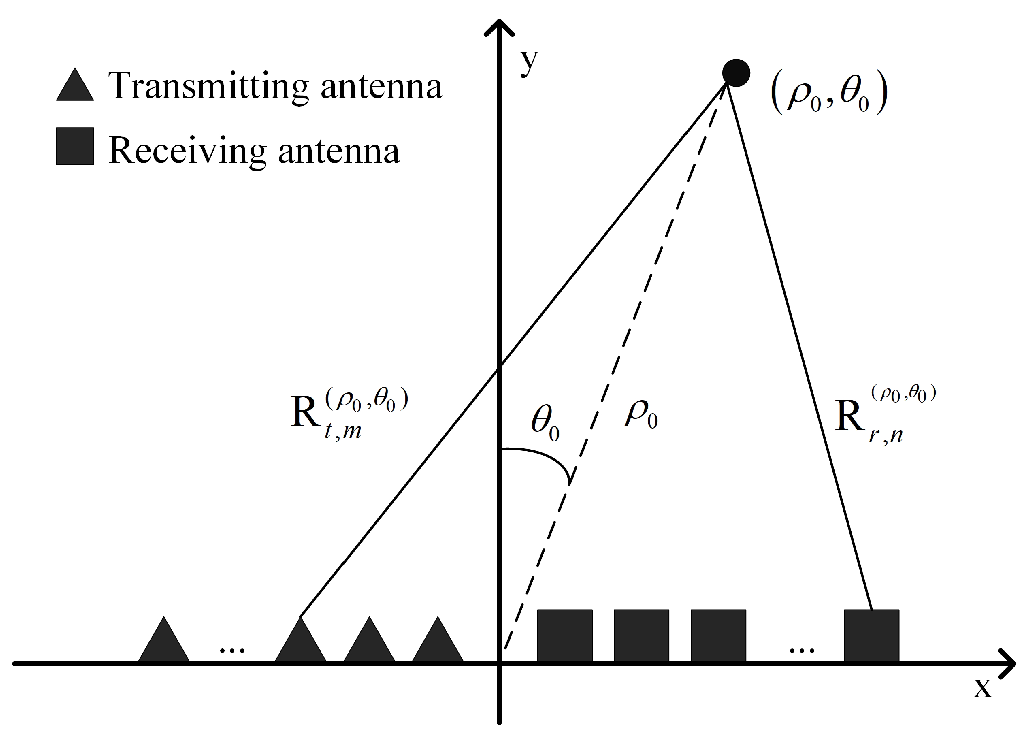
2. MIMO-SAR System and Signal Model

Ground-based MIMO-SAR with multiple transmitting antennas and multiple receiving antennas can form multiple pairs of combined receiving and transmitting channels to obtain a longer equivalent aperture with fewer antennas. The combination of M transmitting units and N receiving units can provide MN equivalent virtual antenna units. In the far field, it can be equated that the signal is transmitted and received by the same virtual antenna unit. However, in the near field, the phase center approximation error needs to be compensated [26,27], as discussed below.

The main parameters of the MIMO-SAR designed by our team are shown in

Table 1. Main parameters of MIMO-SAR system.

Parameter	Value
Carrier frequency	20 GHz
Bandwidth	200 MHz
Number of transmitting antenna	16
Number of receiving antenna	8
Aperture length	0.4064 m
Range	20 m–2000 m
Azimuth angle	$-{45}^{\circ }$–$+{45}^{\circ }$

. The photograph of the radar system used for data collection is shown in Figure 1. The structure of the MIMO-SAR array is shown in Figure 2. The MIMO-SAR system consists of 16 transmitting antennas and 8 receiving antennas. The value of d in Figure 2 is 3.2 mm.

The echo received by MIMO-SAR in a pulse period after range compression can be expressed as

$$s_r\left(t\right)=rect\left(\frac{x}{L}\right)p_r\left(t-(R_{t,m}^{{}^{({\rho }_0,{\theta }_0)}}+R_{r,n}^{{}^{({\rho }_0,{\theta }_0)}})/c\right)·exp\left[-j2\pi f_c(R_{t,m}^{{}^{({\rho }_0,{\theta }_0)}}+R_{r,n}^{{}^{({\rho }_0,{\theta }_0)}})/c\right]$$

(1)

where $rect(x/L)$ is the azimuth envelope, and L is the aperture length. $p_r(\cdot )$ is the compressed range envelope, c is the speed of light, and $f_c$ is the carrier frequency. Suppose the target is located at $\left({\rho }_0,{\theta }_0\right)$, ${\rho }_0$ is the distance from the target to the center of the radar array, ${\theta }_0$ is the angle between the target and the center of the radar array, $R_{t,m}^{{}^{({\rho }_0,{\theta }_0)}}$ is the distance from the m-th transmitting unit to the target, and $R_{r,n}^{{}^{({\rho }_0,{\theta }_0)}}$ is the distance from the n-th receiving unit to the target.

3. Phase Center Approximation Error Analysis and Compensation for MIMO-SAR

The data processing of MIMO-SAR usually adopts an equivalent array to simplify the signal model. However, phase center approximation error will inevitably be introduced in the equivalent array. This error will lead to false peaks in the azimuth compression result, which will seriously affect the imaging quality. In [28], the author analyzes the phase center approximation error in a linear array. In [29], the author analyzes the phase center approximation error in the square boundary array, but the author does not consider the influence of range. In [30], the author analyzes the influence of height differences in a non-collinear array on radar design. In this paper, the phase center approximation error of a non-collinear array is analyzed. First, the phase center approximation error of a linear array is briefly introduced, and then the influence of height difference in a non-collinear array is analyzed. Finally, the phase compensation results are given.

3.1. Phase Center Approximation Error in Linear Array

The principle of the one-dimensional linear array MIMO radar is shown in Figure 3. The MIMO-SAR one-dimensional linear array is composed of M transmitting units and N receiving units, which can provide MN observation channels and increase the freedom of MIMO-SAR to form a longer equivalent aperture. Take the position of the linear equivalent array as the x-axis, denoting the position of the transmitting unit as $x_{t,m}(m=1,2,...,M)$ and the position of the receiving antenna unit as $x_{r,n}(n=1,2,...,N)$. When the radar signal is transmitted from the m-th transmitting unit, reflected by the target $P({\rho }_0,{\theta }_0)$ and then received by the n-th receiving unit, the two distances can be expressed as

$$R_{t,m}^{{}^{({\rho }_0,{\theta }_0)}}=\sqrt{{\rho }_0^2+x_{t,m}^2-2{\rho }_0{x}_{t,m}sin{\theta }_0}$$

(2)

$$R_{r,n}^{{}^{({\rho }_0,{\theta }_0)}}=\sqrt{{\rho }_0^2+x_{r,n}^2-2{\rho }_0{x}_{r,n}sin{\theta }_0}$$

(3)

The corresponding time delay can be expressed as

$${\tau }_{mn}^{({\rho }_0,{\theta }_0)}=\frac{R_{t,m}^{{}^{({\rho }_0,{\theta }_0)}}+R_{r,n}^{{}^{({\rho }_0,{\theta }_0)}}}{c}$$

(4)

For a radar system with separate transmitters and receivers, the virtual array theory demonstrates that it can be equivalent to the virtual antenna unit transmits and receives the signal at the midpoint of the line connecting the transmitting unit and the receiving unit. In the far field, this is reasonable, but in the near field, a phase center approximation error will be introduced in the equivalent array, and this error will lead to false peaks in the azimuth compression result, which will affect the final imaging quality. As shown in Figure 4, when the signal transmitted by the m-th transmitting unit is received by the n-th receiving unit, then the position of the equivalent antenna unit can be expressed as

$$x_k=\frac{x_{t,m}+x_{r,n}}{2},k=1,2,...,MN$$

(5)

Therefore, the distance error caused by the phase center approximation can be calculated. By Taylor expansion and neglecting the high-order terms, it can be expressed as

$$\begin{array}{cc}\hfill \Delta R& =R_{t,m}^{{}^{({\rho }_0,{\theta }_0)}}+R_{r,n}^{{}^{({\rho }_0,{\theta }_0)}}-2R_k^{{}^{({\rho }_0,{\theta }_0)}}\hfill \\ \hfill & =\sqrt{{\rho }_0^2+x_{t,m}^2-2{\rho }_0{x}_{t,m}sin{\theta }_0}+\sqrt{{\rho }_0^2+x_{r,n}^2-2{\rho }_0{x}_{r,n}sin{\theta }_0}\hfill \\ \hfill & -2\sqrt{{\rho }_0^2+x_k^2-2{\rho }_0{x}_{k}sin{\theta }_0}\hfill \\ \hfill & \approx \frac{{cos}^2{\theta }_0}{4{\rho }_0}{(x_{t,m}-x_{r,n})}^2\hfill \end{array}$$

(6)

3.2. Analysis of Non-Collinear Array

In the actual MIMO-SAR system, there is usually a height difference between the transmitting and receiving arrays. The principle of non-collinear array MIMO radar is shown in Figure 5. The position of the equivalent virtual array is taken as the x-axis, denoting the position of the transmitting unit as $x_{t,m}(m=1,2,...,M)$ and the position of the receiving unit as $x_{r,n}(n=1,2,...,N)$. The radar center axis is taken as the z-axis, denoting the position of the transmitting unit as $z_{t,m}(m=1,2,...,M)$ and the position of the receiving unit as $z_{r,n}(n=1,2,...,N)$.

As shown in Figure 6, the error in the non-collinear array can be decomposed into three parts. The first part is the error caused by the virtual transmitting unit, the virtual receiving unit and the equivalent virtual antenna unit. This part of the error caused by the phase center approximation is similar to that of the linear array. The second part is the error caused by the transmitting unit and the virtual transmitting unit, and the third part is the error caused by the receiving unit and the virtual receiving unit.

The phase center approximation error in the non-collinear array is decomposed into three parts: the first part of the error is denoted as $\Delta R_1$, the second part of the error is denoted as $\Delta R_2$, and the third part of the error is denoted as $\Delta R_3$. The geometry relationship between the transmitting unit and the virtual transmitting unit is shown in Figure 7, and the geometry relationship between the receiving unit and the virtual receiving unit is similar. $\Delta R_1$ is calculated similarly to the linear array case; then, $\Delta R_2$ and $\Delta R_3$ can be expressed as

$$\left\{{}_{\Delta R_3=R_{r,n}^{{}^{({\rho }_0,{\theta }_0)}}-R_{r,n^{{}^{\prime }}}^{{}^{({\rho }_0,{\theta }_0)}}\approx \frac{{cos}^2{\phi }_0}{2R_{r,n^{{}^{\prime }}}^{{}^{({\rho }_0,{\theta }_0)}}}{h}^2}^{\Delta R_2=R_{t,m}^{{}^{({\rho }_0,{\theta }_0)}}-R_{t,m^{{}^{\prime }}}^{{}^{({\rho }_0,{\theta }_0)}}\approx \frac{{cos}^2{\phi }_0}{2R_{t,m^{{}^{\prime }}}^{{}^{({\rho }_0,{\theta }_0)}}}{h}^2}\right.$$

(7)

In the case of the non-collinear array, the distance error caused by the phase center approximation can be expressed as

$$\Delta R=\frac{{cos}^2{\theta }_0}{4{\rho }_0}{(x_{t,m}-x_{r,n})}^2+\frac{{cos}^2{\phi }_0}{2R_{t,m^{{}^{\prime }}}^{{}^{({\rho }_0,{\theta }_0)}}}{h}^2+\frac{{cos}^2{\phi }_0}{2R_{r,n^{{}^{\prime }}}^{{}^{({\rho }_0,{\theta }_0)}}}{h}^2$$

(8)

In Equation (8), the distance error changes both with the distance and azimuth angle. However, the azimuth aperture of the MIMO array is usually very short, and the error varies slowly with the azimuth angle. It is enough to focus only on the influence of distance. When the observation angle is $\pm {45}^{\circ }$, taking ${30}^{\circ }$ as the reference center to minimize the residual error, the distance error can be reasonably simplified as

$$\Delta R\approx \frac{{cos}^2\left(\pi /6\right)}{4{\rho }_0}{(x_{t,m}-x_{r,n})}^2+\frac{1}{{\rho }_0}{h}^2$$

(9)

The distance error caused by the height difference in Equation (9) does not change with the switching of the transceiver channel and has no affect on the imaging. Therefore, only the first term in Equation (9) needs to be compensated. The error compensation method is as follows. First, the raw echo data are processed to get the range compression result. Then, for each range bin, the data are compensated according to the positions of the receiving and transmitting array unit. The compensated phase error can be expressed as

$${\varphi }_{\Delta R}=exp\left\{j\frac{2\pi f_c}{c}·\frac{{cos}^2\left(\pi /6\right)}{4{\rho }_0}{(x_{t,m}-x_{r,n})}^2\right\}$$

(10)

After error compensation, the array sampling can be equivalent to virtual array unit sampling, which is convenient for imaging processing. Then, the collected data are rearranged in the order of the virtual array unit. The full aperture echo data after error compensation can be expressed as

$$s_r(\rho ,x)=rect\left(\frac{x}{L}\right)p_r\left(\rho -R(x;{\rho }_0,{\theta }_0)\right)·exp\left[-j4\pi f_{c}R(x;{\rho }_0,{\theta }_0)/c\right]$$

(11)

where $\rho$ is the range sampling, x is the radar location, L is the aperture length, $f_c$ is the carrier frequency, c is the speed of light, and $R(x;{\rho }_0,{\theta }_0)$ is the distance from the current radar location to the target.

In the near field, the phase center approximation error introduces paired sidelobes into the azimuth compression result. In Equation (8), it can be found that the farther the distance and the larger the angle, the smaller the error that needs to be compensated. The simulation parameters are shown in Table 1. Targets are set at $\left(20\mathrm{m},0^{\circ }\right)$ and $\left(20\mathrm{m},-{45}^{\circ }\right)$, and the corresponding azimuth sine values are 0 and −0.707; then, the echo data are compensated by Equation (10). The compensation results are shown in Figure 8 and Figure 9. As shown in the Figure 10, the MIMO-SAR system in this paper consists of 16 transmitting antennas and 8 receiving antennas, which can provide $16\times 8$ observation channels with numbers from 1 to 128. It can be seen that the phase of the target is clearly modulated by the geometry of the radar array before the phase error compensation. The phase error variance of the $0^{\circ }$ target is 0.1 before compensation, and after compensation it is 0.007. The phase error variance of the $-{45}^{\circ }$ target is 0.025 before compensation, and after compensation it is 0.005. After phase error compensation, the paired sidelobes in the azimuth compression result are lower than −45 dB, which meets the imaging requirements.

4. MIMO-SAR Fast Imaging Algorithm

In recent years, ground-based synthetic aperture radar has been widely used in the field of deformation monitoring. A robust, accurate and fast imaging algorithm is required to obtain the real-time deformation of the monitoring area. The imaging geometry of ground-based SAR is different from that of airborne and spaceborne SAR, which will lead to the linear amplification of azimuth resolution with the distance of the target [31]. Therefore, ground-based SAR is more suitable for polar format imaging algorithms. In [32], the author proposes a fast imaging algorithm for subimage coherent synthesis, which can achieve both near-field and far-field imaging. However, the algorithm uses two one-dimensional interpolations to realize the transformation of the coordinate system when obtaining the result of subimage coherent synthesis, which is the main source of the computational cost. In order to solve this problem, this paper proposes the use of two linear transformations instead of two one-dimensional interpolations, further improving the processing efficiency of the algorithm. In the following, the subimage coherent synthesis algorithm using two one-dimensional interpolations is called the interpolation method to distinguish it from the algorithm proposed in this paper.

4.1. The Principle of Subimage Coherent Synthesis Fast Imaging Algorithm Based on Interpolation

The synthetic aperture length of ground-based MIMO-SAR is usually very short, and if the entire synthetic aperture is uniformly divided into several subapertures of shorter length, the signal model inside the subaperture can be reasonably simplified. Figure 11 shows the schematic diagram of the subaperture model. In Figure 11, the position of the n-th subaperture center is $x_n$. We denote the distance between target point P and the n-th subaperture center as ${\rho }_{x_n,0}$, and the azimuth angle between target point P and the n-th subaperture center as ${\theta }_{x_n,0}$. The azimuth variable under the subaperture coordinate system is denoted as $x_{n-0}=x-x_n$, and then the distance between the target point P and the radar can be expressed as

$$\begin{array}{cc}\hfill R(x_{n-0};{\rho }_{x_n,0},{\theta }_{x_n,0})& =\sqrt{{\rho }_{x_n,0}^2+x_{n-0}^2-2{\rho }_{x_n,0}{x}_{n-0}sin{\theta }_{x_n,0}}\hfill \\ \hfill & \approx {\rho }_{x_n,0}-sin{\theta }_{x_n,0}{x}_{n-0}+\frac{(1-{sin}^2{\theta }_{x_n,0})}{2{\rho }_{x_n,0}}{x}_{n-0}^2\hfill \end{array}$$

(12)

Therefore, the echo inside the n-th subaperture can be expressed as

$$\begin{array}{cc}\hfill s_r({\rho }_{n-0},x_{n-0})& =rect\left(\frac{x_{n-0}}{L_{\Delta }}\right)p_r\left({\rho }_{n-0}-{\rho }_{x_n,0}+sin{\theta }_{x_n,0}{x}_{n-0}\right)\hfill \\ \hfill & ·exp\left[-j4\pi f_c{\rho }_{x_n,0}/c+j4\pi f_{c}sin{\theta }_{x_n,0}{x}_{n-0}/c\right]\hfill \\ \hfill & ·exp\left[-j4\pi f_c\left(\frac{(1-{sin}^2{\theta }_{x_n,0})}{2{\rho }_{x_n,0}}{x}_{n-0}^2\right)/c\right]\hfill \end{array}$$

(13)

Equation (13) indicates that the echo has range migration and high-order phase terms. To ensure the focus of targets, the range migration should be smaller than a quarter of the range resolution, and the high-order phase term should be smaller than $\pi /8$. In order to meet the above two conditions, the length of the subaperture $L_{\Delta }$ must be limited.

$$L_{\Delta }\le min\left\{\frac{{\rho }_r}{2sin\left({\left|\theta \right|}_{max}\right)},\frac{\sqrt{{\lambda }_c{\rho }_{min}}}{2}\right\}$$

(14)

The signal model inside the subaperture can be simplified as

$$\begin{array}{cc}\hfill s_r({\rho }_{n-0},x_{n-0})& =rect\left(\frac{x_{n-0}}{L_{\Delta }}\right)p_r\left({\rho }_{n-0}-{\rho }_{x_n,0}\right)\hfill \\ \hfill & ·exp\left[-j4\pi f_c{\rho }_{x_n,0}/c+j4\pi f_{c}sin{\theta }_{x_n,0}{x}_{n-0}/c\right]\hfill \end{array}$$

(15)

Then, there is no range migration inside the subaperture, and the phase history is linear.

The main idea of the subimage coherent synthesis fast imaging algorithm is to divide the entire aperture into several subapertures uniformly and process the subaperture data individually to get coarse resolution subimages. Then, the imaging results in the subaperture coordinate system are converted into the full aperture coordinate system by two one-dimensional interpolations. After coordinate system transformation, the point target appears in the same pixel unit in each subimage. Finally, the full-resolution imaging result can be obtained by the coherent synthesis of subimages.

4.2. A Subimage Coherent Synthesis Algorithm Based on Geometric Transformation

Subimages can be obtained by performing azimuth Fourier transformation on the subaperture data, and the imaging results can be expressed as

$$\begin{array}{cc}\hfill I_n({\rho }_{n-0},sin{\theta }_{x_n,0})& =FFT\left(s_r({\rho }_{n-0},x_{n-0})\right)\hfill \\ \hfill & ={\rho }_a(sin{\theta }_{n-0}-sin{\theta }_{x_n,0})·{\rho }_r({\rho }_{n-0}-{\rho }_{x_n,0})\hfill \\ \hfill & ·exp\left(-j\frac{4\pi f_c{\rho }_{x_n,0}}{c}\right)\hfill \end{array}$$

(16)

As shown in Figure 12, the position of the target point P in the full aperture coordinate system is $({\rho }_0,{\theta }_0)$, and the position offset of the target point P from the subaperture coordinate system to the full aperture coordinate system is denoted as $(\Delta \rho ,\Delta \theta )$, which includes the range offset $\Delta \rho ={\rho }_1-{\rho }_0$ and the angle offset $\Delta \theta ={\theta }_1-{\theta }_0$.

The position of the n-th subaperture center is $x_n$. The transformation relation can be obtained according to the cosine theorem.

$${\rho }_0=\sqrt{{\rho }_1^2+x_n^2-2{\rho }_1{x}_{n}sin\left({\theta }_1\right)}$$

(17)

By truncating the series of Taylor expansion appropriately, the range offset can be expressed as

$${\rho }_1-{\rho }_0=sin\left({\theta }_1\right)x_n$$

(18)

The aperture length of ground-based MIMO-SAR is relatively short, which makes the second-order term in the Taylor expansion very small. With the radar parameters in Table 1, the second-order term is about ${10}^{-4}$, which is far less than a quarter of the range resolution. Therefore, the second-order and higher-order terms can all be ignored. It can be seen from Equation (18) that the range offset is only related to the azimuth angle. Therefore, range translation can be achieved by Inverse Fourier transformation (IFFT), linear phase multiplication and Fourier transformation (FFT). After range translation, the position of target P is converted to $({\rho }_0,{\theta }_1)$, and the range variable of target P relative to the center of the subaperture is converted to the range variable relative to the center of the full aperture.

In the azimuth dimension, the transformation relation can be obtained according to the sine theorem.

$$\frac{x_n}{sin({\theta }_0-{\theta }_1)}=\frac{{\rho }_0}{cos{\theta }_1}$$

(19)

The angle offset can be expressed as

$${\theta }_0-{\theta }_1=arcsin(x_{n}cos{\theta }_1/{\rho }_0)\approx arcsin(x_n/{\rho }_0)$$

(20)

Since $x_n/{\rho }_0$ is very small, the angle rotation after approximation is only related to the distance, Thus, the angle rotation can be achieved by IFFT, linear phase multiplication and FFT. After angle rotation, the position of target P is converted to $({\rho }_0,{\theta }_0)$, and the azimuth variable of target P relative to the subaperture center is converted to the azimuth variable relative to the full aperture center. Then, the imaging results of the subaperture coordinate system are converted into the full aperture coordinate system.

Finally, the transformed subimages are phase compensated and coherently synthesized to obtain the full aperture imaging result. The phase to be compensated for the subimage can be expressed as

$${\phi }_{com}(\rho ,sin\theta )=-\frac{4\pi f_c(R(\rho ,\theta )-R_{x_n}(\rho ,\theta ))}{c}\approx -\frac{4\pi f_c}{c}sin\theta ·x_n$$

(21)

where $R_{x_n}(\rho ,\theta )$ is the distance from the target $(\rho ,\theta )$ to the center of the subaperture. $R(\rho ,\theta )$ is the distance from the target $(\rho ,\theta )$ to the center of the full aperture. The final imaging result can be expressed as

$$\begin{array}{cc}\hfill I(\rho ,sin\theta )& =\sum _{n=1}^N{I}_n(\rho ,sin\theta )\dot{exp}\left(j{\phi }_{com}(\rho ,sin\theta )\right)\hfill \\ \hfill & ={\rho }_a(sin\theta -sin{\theta }_0)·{\rho }_r(\rho -{\rho }_0)·exp\left(-j\frac{4\pi f_c{\rho }_0}{c}\right)\hfill \end{array}$$

(22)

The specific operation of this algorithm are given below. The processing flow chart (with four subapertures) is shown in Figure 13.

• After phase center approximation (PCA) error compensation, the data are rearranged in the order of virtual array elements;
• Then, the rearranged data of each subaperture are extracted and windowed, and the coarse resolution imaging results in the subaperture coordinate system can be obtained;
• The subimages are converted into the full aperture coordinate system by distance translation and angle rotation;
• Finally, the transformed subimages are phase compensated and coherently synthesized to obtain the full resolution imaging result of the scene.

4.3. The Computational Cost Analysis of the Algorithm

In order to analyze the computational cost of the proposed method and compare it with the interpolation method, the algorithm is decomposed step by step, and the number of multiplication, addition and other operations required for each step is analyzed. The process of obtaining coarse resolution subimages is the same, so the computational cost is not considered; only the number of operations required for azimuth imaging is analyzed.

We assume that the full aperture is divided into n subapertures and the image size is $N_a·N_r$, $N_a$ is the azimuth data size, and $N_r$ is the range data size. The analyses of the interpolation method are as follows:

• For a single pixel, the azimuth coordinate mapping is calculated, and then the interpolation calculation is applied. It is assumed that the FFT interpolation algorithm is used. The processing of a pixel requires six multiplications, four additions and one square root. A total of $n·N_a·N_r$ pixels need to be processed;
• For a single pixel, the range coordinate mapping is calculated, and then the interpolation calculation is applied. The processing of a pixel requires eight multiplications, six additions and one square root. A total of $n·N_a·N_r$ pixels need to be processed;
• For a single pixel, the compensation phase is calculated. The processing of a pixel requires two multiplications. A total of $n·N_a·N_r$ pixels need to be processed;
• Finally, the phase compensation and coherent synthesis of subimages require $n·N_a·N_r$ multiplications and $n·N_a·N_r$ additions.

For the convenience of comparison, the case of a single pixel is also considered when analyzing the proposed method. The specific analysis of the methods proposed in this paper is as follows:

• For a single pixel, the range offset is calculated according to Equation (18). Range translation is realized by linear phase multiplication. The processing of a pixel requires two multiplications. A total of $n·N_a·N_r$ pixels need to be processed;
• For a single pixel, the angle offset is calculated according to Equation (20). Angle rotation is realized by linear phase multiplication. The processing of a pixel requires two multiplications. A total of $n·N_a·N_r$ pixels need to be processed;
• For a single pixel, the compensation phase is calculated according to Equation (21). The processing of a pixel requires two multiplications. A total of $n·N_a·N_r$ pixels need to be processed;
• Finally, the phase compensation and coherent synthesis of subimages require $n·N_a·N_r$ multiplications and $n·N_a·N_r$ additions.

As shown in

Table 2. Computational cost analysis.

Operational Method	Interpolation Method	The Method Proposed in This Paper
Multiplication	$17·n·N_a·N_r$	$7·n·N_a·N_r$
addition	$12·n·N_a·N_r$	$n·N_a·N_r$
square root	$2·n·N_a·N_r$	0

, the method proposed in this paper replaces the complex interpolation operation by linear multiplication, which greatly reduces the number of operations required for azimuth imaging, and the number of operations decreases with the increase of the number of subapertures. Therefore, the computational cost of the proposed method in this paper is much lower than the interpolation method, and it has better real-time performance.

5. Simulation and Experiment

5.1. Simulation

The subimage coherent synthesis algorithm based on geometric transformation proposed in this paper is used to process the near-field single point target simulation data, The results are shown in Figure 14, and the focusing performance comparison is shown in Figure 15. The simulation parameters are shown in Table 1. Then, the single point target is set at $(20\mathrm{m},45{}^{\circ })$, and the corresponding azimuth sine value is 0.707. The two-dimensional resolution and peak sidelobe ratio of the imaging results are shown in

Table 3. Point target performance analysis.

Performance Criteria	Measured Value Based on Interpolation Method	Measured Value of the Method Proposed in This Paper
Range resolution	0.75 m	0.75 m
Azimuth resolution	0.015	0.015
Range PSLR	−13.38 dB	−13.38 dB
Azimuth PSLR	−13.15 dB	−13.16 dB

. The simulation results show that both images are focused well.

5.2. Experiment

In this section, an in-site experiment result is presented. The data are collected at an open pit mine, in the ChangSha province of China. The instrument is a Ka-band frequency modulated continuous wave radar system with a bandwidth of 200 MHz. The azimuthal synthetic aperture length of the system is 0.4064 m. In Figure 16, the observed scene is shown. The slope is located at the range from 200 to 500 m. Some buildings are situated at about 600 m. The typical structures are clearly imaged in the imaging results. Figure 17 shows the imaging results. The strongly scattered targets marked by red circles in Figure 17 are selected for analysis. As shown in Figure 18 and Figure 19, the two algorithms have similar focusing performance. The phase difference of the target in the two imaging results is 0.0081 rad, and the results are shown in

Table 4. Point target performance analysis.

Performance Criteria	Measured Value Based on Interpolation Method	Measured Value of the Method Proposed in This Paper
Range resolution	0.89 m	0.89 m
Azimuth resolution	0.018	0.018
Range PSLR	−24.35 dB	−24.37 dB
Azimuth PSLR	−26.81 dB	−26.84 dB

. Since the Hamming window has been applied in the range frequency and azimuth aperture domain, the main lobe of the target is about 1.2 times wider. The phase difference between the two imaging results is smaller than 0.01 rad. The time cost of the subimage coherent synthesis imaging algorithm based on two one-dimensional interpolations is about 12 s, while the subimage coherent synthesis imaging algorithm based on geometric transformation needs 6 s only.

6. Conclusions

In this paper, a fast imaging algorithm tailored for ground-based MIMO-SAR data is proposed, which can be applied in both far-field and near-field scenarios. First, the phase center approximation error of the non-collinear array in the near field is analyzed. Then, a fast imaging algorithm based on geometric transformation for the coherent synthesis of subimages is put forward. First, the phase center approximation error of MIMO-SAR is compensated, and then the full aperture is divided into several subapertures according to the subaperture division conditions, in which the influence of range migration and high-order phase terms on focusing imaging can be ignored. The efficiency of the algorithm can be further improved by using two linear multiplications instead of two one-dimensional interpolations without affecting the imaging quality. After the geometric transformation, the subimages are transformed into a full aperture coordinate system, and the full aperture resolution imaging results can be obtained by the coherent synthesis of subimages. This algorithm can deal with both near and far-field MIMO-SAR data and obtains the imaging results in a pseudopolar coordinate system. The algorithm is extensively validated with simulation data and measured data.

References

1. Wang, Y.; Hong, W.; Zhang, Y.; Lin, Y.; Li, Y.; Bai, Z.; Zhang, Q.; Lv, S.; Liu, H.; Song, Y. Ground-Based Differential Interferometry SAR: A Review. IEEE Geosci. Remote Sens. Mag. 2020, 8, 43–70. [Google Scholar] [CrossRef]
2. Pieraccini, M.; Miccinesi, L. Ground-Based Radar Interferometry: A Bibliographic Review. Remote Sens. 2019, 11, 1029. [Google Scholar] [CrossRef] [Green Version]
3. Caduff, R.; Schlunegger, F.; Kos, A.; Wiesmann, A. A review of terrestrial radar interferometry for measuring surface change in the geosciences. Earth Surf. Process. Landforms 2015, 40, 208–228. [Google Scholar] [CrossRef]
4. Zhou, Z.; Cheng, X.; Zhou, W.; Hao, W.; Xiao, H.; Chen, H.; Yang, K. Application of GB-SAR in landslide deformation monitoring. Bull. Surv. Mapp. 2022, 7, 60–63. Available online: http://tb.chinasmp.com/EN/10.13474/j.cnki.11-2246.2022.0204 (accessed on 16 January 2023).
5. Tarchi, D.; Rudolf, H.; Luzi, G.; Chiarantini, L.; Sieber, A.J. SAR interferometry for structural change detection: A demonstration test on a dam. In Proceedings of the International Geoscience and Remote Sensing Symposium, IGARSS ’99 Proceedings, Hamburg, Germany, 28 June–2 July 1999; Volume 3, pp. 1522–1524. [Google Scholar]
6. Martinez-Vazquez, A.; Fortuny-Guasch, J. A GB-SAR Processor for Snow Avalanche Identification. IEEE Trans. Geosci. Remote Sens. 2008, 46, 3948–3956. [Google Scholar] [CrossRef]
7. Nico, G.; Leva, D.; Antonello, G.; Tarchi, D. Ground-based SAR interferometry for terrain mapping: Theory and sensitivity analysis. IEEE Trans. Geosci. Remote Sens. 2004, 42, 1344–1350. [Google Scholar] [CrossRef]
8. Luo, Y.; Song, H.; Wang, R.; Deng, Y.; Zhao, F.; Xu, Z. Arc FMCW SAR and Applications in Ground Monitoring. IEEE Trans. Geosci. Remote Sens. 2014, 52, 5989–5998. [Google Scholar] [CrossRef]
9. Roedelsperger, S.; Becker, M.; Gerstenecker, C.; Laeufer, G.; Schilling, K.; Steineck, D. Digital elevation model with the ground-based SAR IBIS-L as basis for volcanic deformation monitoring. J. Geodyn. 2010, 49, 241–246. [Google Scholar] [CrossRef] [Green Version]
10. Fishler, E.; Haimovich, A.; Blum, R.; Chizhik, D.; Cimini, L.; Valenzuela, R. MIMO radar: An idea whose time has come. In Proceedings of the IEEE Radar Conference, Philadelphia, PA, USA, 26–29 April 2004; pp. 71–78. [Google Scholar] [CrossRef] [Green Version]
11. Zeng, T.; Deng, Y.; Hu, C.; Tian, W. Development and application examples of ground-based differential interferometric radar. J. Radars 2019, 8, 154–170. [Google Scholar] [CrossRef]
12. Tarchi, D.; Oliveri, F.; Sammartino, P.F. MIMO Radar and Ground-Based SAR Imaging Systems: Equivalent Approaches for Remote Sensing. IEEE Trans. Geosci. Remote Sens. 2013, 51, 425–435. [Google Scholar] [CrossRef]
13. You, Y. Design and Implementation of C-Band Ground-Based MIMO Deformation Monitoring Radar. Ph.D. Thesis, Chongqing University, Chongqing, China, 2021. [Google Scholar]
14. Gao, L.; Zeng, Y.; Zheng, G. Current status and development trend of MIMO radar imaging. Aerosp. Electron. Warf. 2013, 29, 4. [Google Scholar]
15. Pang, B.; Xing, S.; Dai, D.; Li, Y.; Wang, X. Development and perspective of MIMO-SAR imaging technology. Syst. Eng. Electron. 2020, 42, 13. [Google Scholar]
16. Han, X.; Hu, W.; Yu, W.; Du, X. Distributed multi-channel radar imaging technology. J. Electron. Inf. Technol. 2007, 29, 2357–2358. [Google Scholar]
17. Wang, H.; Su, Y.; Zhu, Y.; Xu, H. Research on MIMO radar imaging based on spatial spectral domain filling. Acta Electron. Sin. 2009, 37, 1242–1246. [Google Scholar]
18. Zhuge, X.; Yarovoy, A.G.; Savelyev, T.; Ligthart, L. Modified Kirchhoff Migration for UWB MIMO Array-Based Radar Imaging. IEEE Trans. Geosci. Remote Sens. 2010, 48, 2692–2703. [Google Scholar] [CrossRef]
19. Guccione, P.; Zonno, M.; Mascolo, L.; Nico, G. Focusing algorithms analysis for Ground-Based SAR images. In Proceedings of the 2013 IEEE International Geoscience and Remote Sensing Symposium—IGARSS, Melbourne, Australia, 21–26 July 2013; pp. 3895–3898. [Google Scholar] [CrossRef]
20. Monti Guarnieri, A.; Scirpoli, S. Efficient Wavenumber Domain Focusing for Ground-Based SAR. IEEE Geosci. Remote Sens. Lett. 2010, 7, 161–165. [Google Scholar] [CrossRef]
21. Wang, H. Research on MIMO Radar Imaging Algorithm. Ph.D. Thesis, National University of Defense Technology, Changsha, China, 2010. [Google Scholar]
22. Gu, F.; Chi, L.; Zhang, Q.; Zhu, F. Single snapshot imaging method in multiple-input multiple-output radar with sparse antenna array. IET Radar Sonar Navig. 2013, 7, 535–543. [Google Scholar] [CrossRef]
23. Jiang, L.; Yang, Z.; Che, L. A Sparse Imaging Algorithm for Time-Division MIMO Landslide Radar. Radar Sci. Technol. 2019, 17, 1–7. [Google Scholar] [CrossRef]
24. Marks, D.L.; Yurduseven, O.; Smith, D.R. Fourier Accelerated Multistatic Imaging: A Fast Reconstruction Algorithm for Multiple-Input-Multiple-Output Radar Imaging. IEEE Access 2017, 5, 1796–1809. [Google Scholar] [CrossRef]
25. Mei, H.; Tian, W.; Hu, C.; Long, T. Fast Imaging Algorithm Based on Ground-Based MIMO Radar. J. Signal Process. 2019, 35, 9. [Google Scholar] [CrossRef]
26. Wang, L.; Xu, J.; HuangFu, K.; Peng, Y. Error bound of MIMO-SAR equivalent phase center based on image quality evaluation. J. Tsinghua Univ. Technol. 2010, 50, 586–590. [Google Scholar]
27. Guo, Y. Imaging Processing and Error Compensation of Airborne Multi-Channel SAR System. Ph.D. Thesis, Xidian University, Xi’an, China, 2017. [Google Scholar]
28. Zhang, X.; Gu, H.; Su, W. Research on Sparse Array Design for UWB MIMO Near-field Imaging Radar. Fire Control. Radar Technol. 2019, 48, 6. [Google Scholar] [CrossRef]
29. Meng, X.; Wu, S.; Tu, H.; Liu, T.; Jin, X. A fast imaging algorithm for sparse array imaging based on PCA and modified SLIM methods. J. Infrared Millim. Waves 2020, 39, 300–305. [Google Scholar] [CrossRef]
30. Cheng, H.; Jingyang, W.; Weiming, T.; Tao, Z.; Rui, W. Design and Imaging of Ground-Based Multiple-Input Multiple-Output Synthetic Aperture Radar (MIMO SAR) with Non-Collinear Arrays. Sensors 2017, 17, 598. [Google Scholar]
31. Monserrat, O.; Crosetto, M.; Luzi, G. A review of ground-based SAR interferometry for deformation measurement. ISPRS J. Photogramm. Remote Sens. 2014, 93, 40–48. [Google Scholar] [CrossRef] [Green Version]
32. Mao, C.; Hu, C.; Zeng, T.; Tian, W. Ground-based SAR Fast imaging Algorithm Based on Sub-image Combination. J. Signal Process. 2015, 31, 1396–1403. [Google Scholar]
Figure 1. Photograph of MIMO-SAR.
Electronics 12 01466 g001
Figure 2. Structure of MIMO-SAR array.
Electronics 12 01466 g002
Figure 3. Geometric model of data collection for one-dimensional linear array MIMO radar.
Electronics 12 01466 g003
Figure 4. Phase center approximation in one-dimensional linear array.
Electronics 12 01466 g004
Figure 5. Geometric model of data collection for non-collinear array MIMO radar.
Electronics 12 01466 g005
Figure 6. Phase center approximation in non-collinear array.
Electronics 12 01466 g006
Figure 7. Schematic diagram of transmitting unit and virtual transmitting unit.
Electronics 12 01466 g007
Figure 8. 20 m , 0 Target compensation result. (a) Phase error before compensation. (b) Phase error after compensation. (c) Azimuthal profile.
Electronics 12 01466 g008
Figure 9. 20 m , 45 Target compensation result. (a) Phase error before compensation. (b) Phase error after compensation. (c) Azimuthal profile.
Electronics 12 01466 g009
Figure 10. Equivalent observation channels diagram.
Electronics 12 01466 g010
Figure 11. Subaperture geometric model of ground-based SAR.
Electronics 12 01466 g011
Figure 12. Schematic diagram of geometric transformation.
Electronics 12 01466 g012
Figure 13. The processing flow chart.
Electronics 12 01466 g013
Figure 14. Imaging results of point target simulation. (a) Imaging results based on interpolation method. (b) Imaging results of the method proposed in this paper.
Electronics 12 01466 g014
Figure 15. Point target profile. (a) Range profile. (b) Azimuthal profile.
Electronics 12 01466 g015
Figure 16. Experimental scene.
Electronics 12 01466 g016
Figure 17. Imaging results of measured data. (a) Imaging results based on interpolation method. (b) Imaging results of the method proposed in this paper.
Electronics 12 01466 g017
Figure 18. Target analysis of imaging results based on interpolation method. (a) Range profile. (b) Azimuthal profile.
Electronics 12 01466 g018
Figure 19. Target analysis of imaging results based on the method proposed in this paper. (a) Range profile. (b) Azimuthal profile.
Electronics 12 01466 g019