Article

Analysis of the Terminal Response Characteristics of the Twisted Three-Wire Cable Excited by a Plane Wave Field

National Key Laboratory on Electromagnetic Environmental Effects, Shijiazhuang Campus of Army Engineering University, Shijiazhuang 050003, China
*
Author to whom correspondence should be addressed.
Electronics 2023, 12(9), 2018; https://doi.org/10.3390/electronics12092018
Submission received: 30 March 2023 / Revised: 20 April 2023 / Accepted: 24 April 2023 / Published: 26 April 2023

Abstract

:
A twisted three-wire cable model with uniform twisting characteristics is proposed in this paper, and its terminal response under external electromagnetic wave irradiation is calculated using the TLM method based on Taylor model. The triple-stranded triple-helix structure is determined in the method and the parametric equations of the twisted wire bundle in the Cartesian coordinate system are provided. Then, the frequency domain equations for the voltage and current of the twisted three-wire cable under field-to-wire coupling are derived and extended to apply to scenarios with arbitrary polarization and irradiation in the incident direction based on the transmission-line theory. Finally, the response laws of the twisted three-wire wire with different cable lengths, termination loads, and pitches coupling under external electromagnetic wave irradiation are studied. A uniform twisted three-wire cable can suppress the increased induced current on the cable. In addition, the excellent characteristics of the twisted three-wire cable in terms of immunity to electromagnetic interference are also verified by comparing the frequency domain response with that of a parallel three-wire cable.

1. Introduction

With the enhancement of electronic equipment intelligence, the impact of external electromagnetic interference becomes more serious. Interference can be coupled with the device through the cable, interfering with the internal control signals, causing abnormalities of the device, or causing breakdown and destruction of the internal circuit chips. Therefore, it is of great significance to investigate the coupling response law of the cables to improve the electromagnetic protection ability of related devices [1,2,3].
Due to their excellent immunity to interference and price advantage, twisted cables are widely used in data transmission tasks such as power transmission cables and automatic control of unmanned aircraft. The principle of the twisted-pair cable anti-interference is reduction in the coupling of the cable with the electromagnetic interference by twisting the conductors into pairs to eliminate the interaction of external electromagnetic fields. Most of these devices use twisted wire for internal data transmission. For devices such as UAVs equipped with brushless motors, the electronic governor and the twisted three-wire cable on the motor are used to issue commands to the motor and control its flight state [4].
Compared to the more straightforward structure of parallel cables, coaxial lines, etc., twisted wires have been investigated by only a few researchers for the field-to-wire coupling associated with twisted wires due to the complexity of their physical structure and coupling laws. Taylor et al. proposed using a double helix model to analyze the coupling characteristics of twisted pair transmission lines under different termination loads [5]. Armenta et al. obtained the analytical form and experimental verification of the termination current of a single TWP under incident field irradiation and generalized it to obtain analytical solutions about TWP bundles [6,7]. Pignari et al. derived an approximate solution for the terminal response of a TWP with uniform and non-uniform pitch in the infinite ground plane and used a circuit model to explain the coupling mechanism of the TWP on the ground [8,9,10]. Yuan et al. used the transmission-line macro model and SPICE circuit model to quickly solve the irradiation response of a twisted pair under terminated nonlinear load. They derived a closed expression for the equivalent modal source considering field-line coupling by examining the actual situation of the dielectric coating around the twisted pair [11,12,13]. Oussama Gassab et al. proposed equations to calculate the per-unit-length parameters of the cable bundle to obtain the coupling equation for a twisted wire bundle above the ground [14,15].
However, the field-to-wire coupling of the twisted three-wire cable has not been modeled in these studies. The high-power microwave (HPM) radiation experiments carried out by our group on UAVs in the early stage have verified that the twisted three-wire cable that controls the operating state of the motor is the main energy coupling path from HPM. The coupling voltage induced on the cables enters the control signal port through the parasitic capacitor and damages the vulnerable parts [16]. Compared with twisted pairs, the structure of the twisted three-wire cable is complex, and effective models are needed to analyze their electromagnetic response and coupling laws in complex electromagnetic environments.

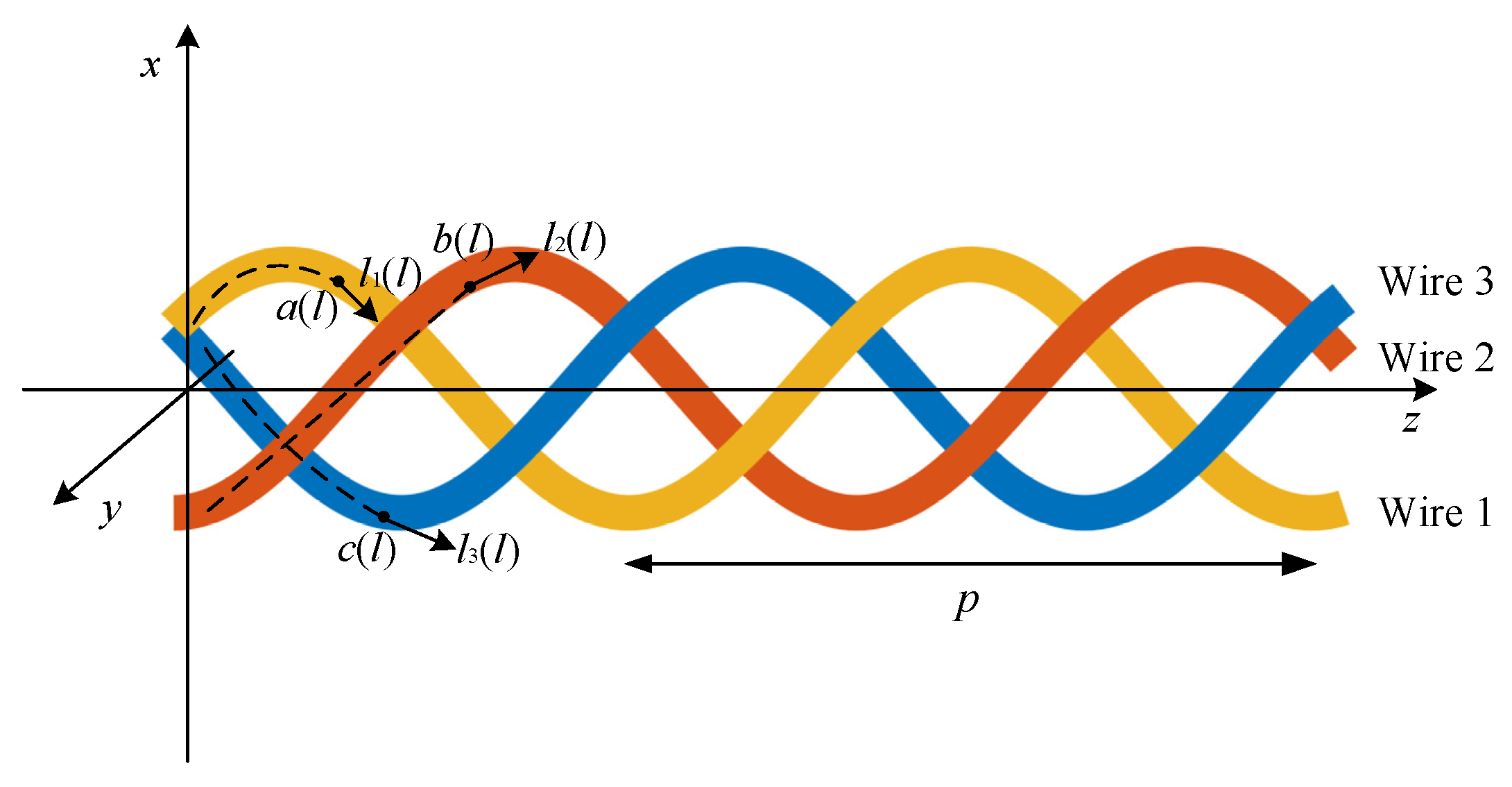
2. The Twisted Three-Wire Cable Triple Helix Structure Model

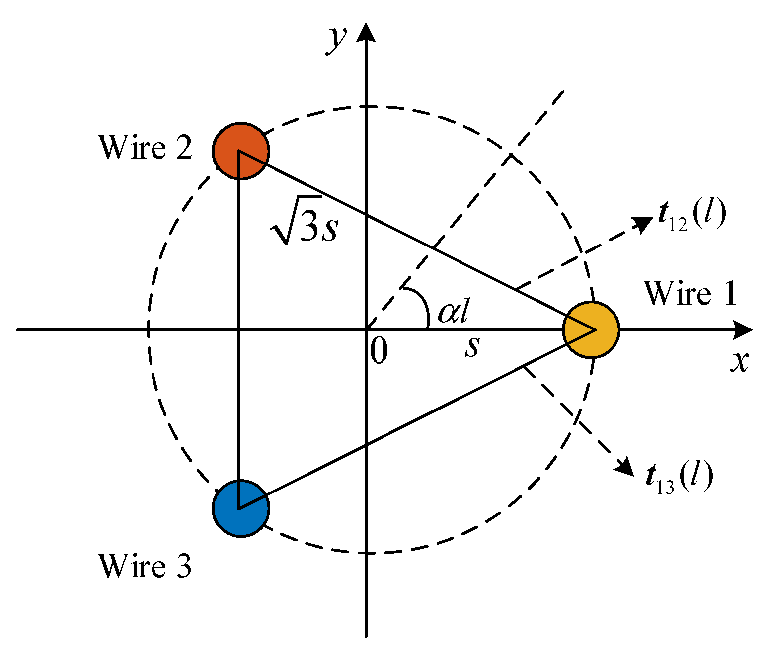
2.1. Twisted Three-Wire Cable Model in Cartesian Coordinate System

The geometry of the twisted three-wire cable can be considered a spiral formed by twisting three conductors. l is the arc length of the wire, which can be obtained from l = 2 π l 0 / p α , and l0 is the length of the twisted three wire cable along the z-axis. The cable is placed along the z-axis and represents the interval between the three lines and the origin. Therefore, the separation distance between the two of the three strands is 3 s , and p represents the pitch of the twisted three-wire cable.
The starting coordinates of the triple helix structure are shown in Figure 1. The Cartesian coordinates of wire 1, wire 2, and wire 3 of the triple helix can be expressed after parameterizing the position coordinates of the three wires as
x 1 ( l ) = s cos ( α l ) , y 1 ( l ) = s sin ( α l ) , z 1 ( l ) = p α l 2 π ,
x 2 ( l ) = s cos ( α l + 2 π / 3 ) , y 2 ( l ) = s sin ( α l + 2 π / 3 ) , z 2 ( l ) = p α l 2 π ,
x 3 ( l ) = s cos ( α l + 4 π / 3 ) , y 3 ( l ) = s sin ( α l + 4 π / 3 ) , z 3 ( l ) = p α l 2 π .
Therefore, the unit vectors t 12 ( l ) , t 13 ( l ) of wire 2 and wire 3 pointing to wire 1 are
t 12 ( l ) = sin ( α l + 60 ° ) a x + cos ( α l + 60 ° ) a y ,
t 13 ( l ) = sin ( α l + 120 ° ) a x + cos ( α l + 120 ° ) a y .
α is known as the twisted three-wire cable rotation parameter, which is defined as
α = ( s 2 + ( p 2 π ) 2 ) 1 .

2.2. Unit Vector of the Twisted Three-Wire Cable

Wire 1 is the reference wire, and the unit vectors l 1 ( l ) , l 2 ( l ) , and l 3 ( l ) are the tangential vectors of wire 1, wire 2, and wire 3 at points a(l), b(l), and c(l), respectively.
As shown in Figure 2, the tangential direction vectors at any point on the twisted three-wire cable are
l 1 ( l ) = s α sin ( α l ) a x + s α cos ( α l ) a y + α p 2 π a z ,
l 2 ( l ) = s α sin ( α l + 2 π / 3 ) a x + s α cos ( α l + 2 π / 3 ) a y + α p 2 π a z ,
l 3 ( l ) = s α cos ( α l + 4 π / 3 ) a x + s α cos ( α l + 4 π / 3 ) a y + α p 2 π a z .

3. The Twisted Three-Wire Cable Terminal Response

3.1. Transmission-Line Equations of the Twisted Three-Wire Cable

Referring to the derivation of the two-conductor transmission-line equations under incident field irradiation, we derive the first frequency domain transmission-line equations for the twisted three-wire cable as [17].
d d l V ( l ) + R I ( l ) + j w L I ( l ) = V F ( l ) ,
V F ( l ) = j w a ( l ) b ( l ) B inc a n d l ,
where V ( l ) and I ( l ) are the matrices of voltages and currents for each line; V F ( l ) is the matrix of distributed voltage sources resulting from the incident electromagnetic field excitation of the transmission line. R is the unit length resistance matrix, and L is the unit length inductance matrix. B inc is the magnetic flux density of the incident field. Similarly, the second transmission-line equations are
d d l I ( l ) + G V ( l ) + j w C V ( l ) = I F ( l ) ,
I F ( l ) = Y a ( l ) b ( l ) E inc ( x , y , z ) d t ( l ) ,
where G is the per-unit-length conductance, C is the per-unit-length capacitance, and I F ( l ) is the matrix of distributed current sources generated by the incident electromagnetic field exciting the transmission line. According to Equations (11) and (13), the per-unit-length voltage and current sources are the incident field’s magnetic and electric field portions, respectively. Thus, the portion of the voltage source can be expressed as
V F ( l ) = d d l [ E 12 T ( l ) E 13 T ( l ) ] + [ E 12 L ( l ) E 13 L ( l ) ] = d d l [ a ( l ) b ( l ) E inc ( x , y , z ) d t 12 ( l ) a ( l ) c ( l ) E inc ( x , y , z ) d t 13 ( l ) ] + [ E inc ( x 2 ( l ) , y 2 ( l ) , z 2 ( l ) ) l 2 ( l ) E inc ( x 1 ( l ) , y 1 ( l ) , z 1 ( l ) ) l 1 ( l ) E inc ( x 3 ( l ) , y 3 ( l ) , z 3 ( l ) ) l 3 ( l ) E inc ( x 1 ( l ) , y 1 ( l ) , z 1 ( l ) ) l 1 ( l ) ] .
E inc is the electric field vector of the incident electromagnetic field. E 12 T ( l ) and E 13 T ( l ) are the contributions of the electric field components in the transverse or z-direction on wire 2 and 3, respectively. The differential vector dt is a column coordinate in the radial direction.

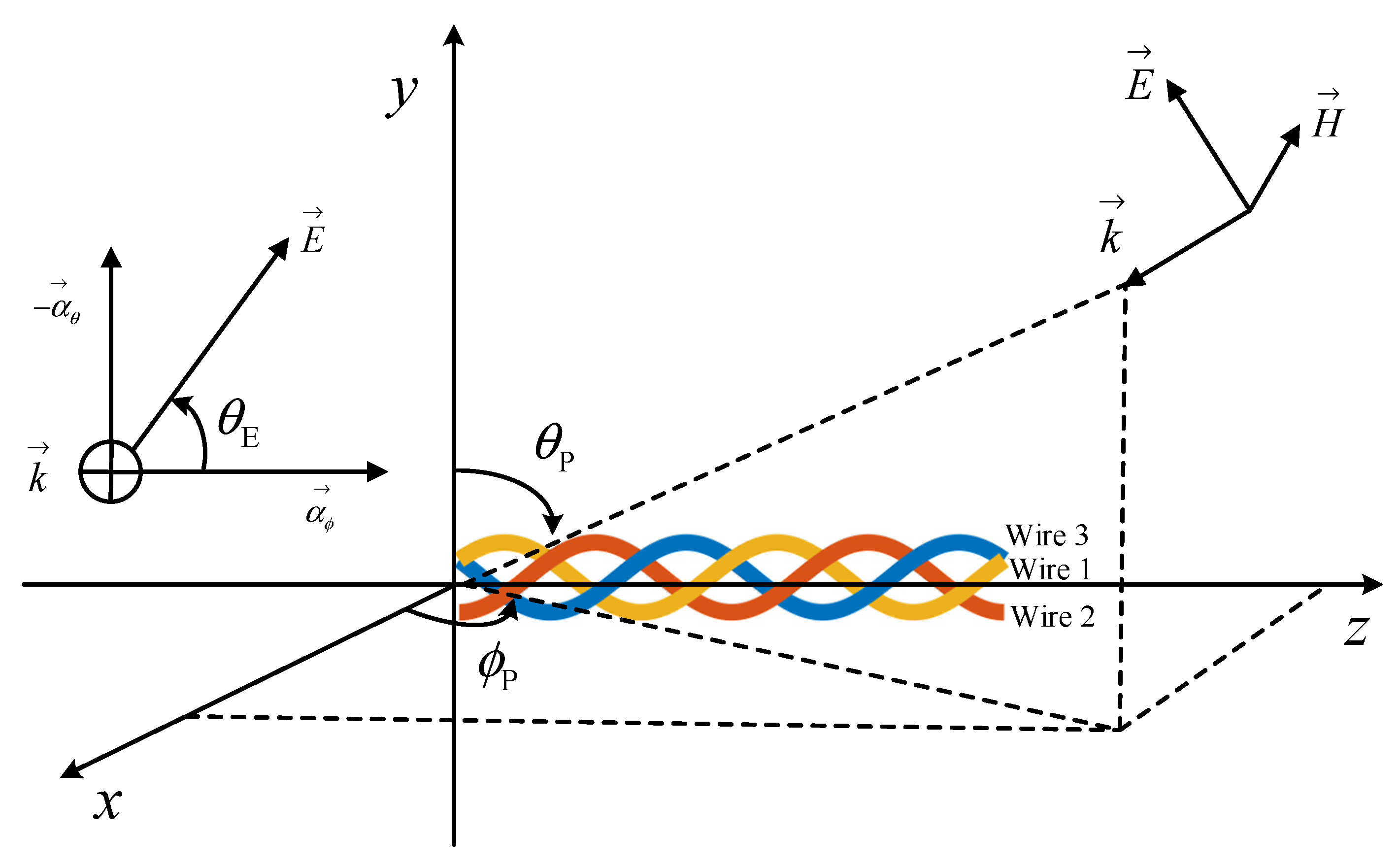
3.2. Plane-Wave Excitation

In the far-field region, the external incident wave can be regarded as a uniform plane wave, and the incident plane wave electric field is expressed as
E inc ( x , y , z ) = E inc ( e x a x + e y a y + e z a z ) e j ( k x x + k y y + k z z ) ,
where E inc is the magnitude of the incident electric field. ex, ey, and ez are the components of the incident field electric field vector in the direction of the x, y, and z axes of the right-angle coordinate system, respectively. kx, ky, and kz are the components of the wavenumber.
These variables can be expressed by the following Equations (16)–(18), where k is the propagation constant of the electromagnetic wave in vacuum pointing to the origin of the coordinates; w is the angular frequency of the plane-wave; λ is the wavelength of the plane-wave; c 0 is the speed of light in vacuum.
{ e x = sin ( θ E ) sin ( θ P ) e y = sin ( θ E ) cos ( θ P ) cos ( ϕ P ) cos ( θ E ) sin ( ϕ P ) e z = sin ( θ E ) cos ( θ P ) sin ( ϕ P ) + cos ( θ E ) cos ( ϕ P ) ,
{ k x = k cos ( θ P ) k y = k sin ( θ P ) cos ( ϕ P ) k z = k sin ( θ P ) sin ( ϕ P ) ,
k = w c 0 = 2 π λ = w μ 0 ε 0 .
A schematic diagram of the incident uniform plane-wave is given in Figure 3. H is the magnetic field vector of the incident electromagnetic field. θ P is the angle between the incident direction and the y-axis, defined as the pitch angle of the incident wave; ϕ P is the angle between the projection of the incident direction in the xoz plane and the x-axis, defined as the azimuth angle of the incident wave; θ E is the angle of polarization expressed by α θ and α ϕ in the spherical coordinate system.

3.3. Terminal Response of the Twisted Three-Wire Cable Equations

The transmission line can be considered a multi-port circuit, and the relationship between the voltage and current at the ports can be characterized by the port parameters. The chain-parameter matrix Φ ( l 0 ) of the twisted three-wire cable is expressed as follows:
Φ ( l 0 ) = [ Φ 11 Φ 12 Φ 21 Φ 22 ] = [ cos ( β l 0 ) 1 2 j sin ( β l 0 ) Z c j v sin ( β l 0 ) Z c 1 cos ( β l 0 ) 1 2 ] ,
where (19) is the 2 × 2 unit matrix, l0 is the arc length of the twisted three-wire cable, and Z c is the characteristic impedance matrix, Z c = v L , Z c 1 = v C . The self-capacitance and self-inductance of the twisted three-wire cable are equal because of the symmetrical structure. Then, the unit length parameter matrixes L and C can be expressed as
L = [ l l m l m l ] = [ μ π ln ( 3 s r ) μ 2 π ln ( 3 s r ) μ 2 π ln ( 3 s r ) μ π ln ( 3 s r ) ] ,
C = μ 0 ε 0 L 1 .
The terminal current is then obtained by combining the terminal constraint in generalized Davinan equivalent form, which can be expressed as
{ I ( 0 ) = [ Φ 11 Z S + Z L Φ 22 Φ 12 Z L Φ 21 Z S ] - 1 ( [ Φ 11 Z L Φ 21 ] V S V L + [ V FT ( l ) Z L I FT ( l ) ] )       I ( l ) = I FT ( l ) + Φ 21 V S + [ Φ 22 Φ 21 Z S ] I ( 0 ) ,
where the pitch p and wavelength λ are much larger than the separation distance 3 s ; Therefore, a simplified method of Taylor’s analysis can be used. To solve the problem by using transmission-line theory, it is necessary to satisfy that the cross-sectional dimensions of the transmission line are electrically small with respect to the incident wavelength λ , where λ = c 0 / f (c0 is the speed of light and f is the frequency).
Due to the fact that the twisted three-wire cable is not straight, there are longitudinal components of the electric and magnetic fields. However, suppose the transverse dimension of the transmission line is much smaller than the incident wave wavelength. In that case, the electromagnetic field components along the incident wave direction are much smaller than the transverse components, and the resulting field can be assumed to be quasi-TEM. It is also necessary to meet the condition that the cable length is much larger than the conductor spacing l 3 s and the conductor spacing is much larger than the conductor radius 3 s r . Otherwise, the wire can be equated to a loop antenna rather than a transmission line.
Eventually, the analytical equations of the induced currents at l = 0 and l = l 0 for a uniform twisted three-wire cable at arbitrarily polarized plane wave incidence are obtained as
I ( 0 ) = [ cos ( β l 0 ) ( Z S + Z L ) + j v sin ( β l 0 ) ( L + Z L C Z S ) ] 1       [ [ cos ( β l 0 ) 1 n + j v sin ( β l 0 ) Z L C ] V S V L       + 0 l 0 { cos ( β ( l 0 τ ) ) 1 n + j v sin ( β ( l 0 τ ) ) Z L C } × [ E 12 L ( τ ) E 13 L ( τ ) ] d τ       [ E 12 T ( l ) E 13 T ( l ) ] z = l 0 + ( cos ( β l 0 ) 1 n + j v sin ( β l 0 ) Z L C ) [ E 12 T ( l ) E 13 T ( l ) ] z = 0 ] ,
I ( l ) = - j v sin ( β l 0 ) C V S + [ cos ( β l 0 ) 1 n + j v sin ( β l 0 ) C Z S ] I ( 0 )   0 l 0 { j v sin ( β ( l 0 τ ) ) C } × [ E 12 L ( τ ) E 13 L ( τ ) ] d τ { j v sin ( β l 0 ) C } [ E 12 T ( l ) E 13 T ( l ) ] z = 0 ,
where Z S and Z L are the impedances of the twisted three-wire cable at l = 0 and l = l 0 , respectively, which can be expressed as
Z S = [ Z S 11 Z S 12 Z S 21 Z S 22 ] Z L = [ Z L 11 Z L 12 Z L 21 Z L 22 ] .

4. Simulation Verification

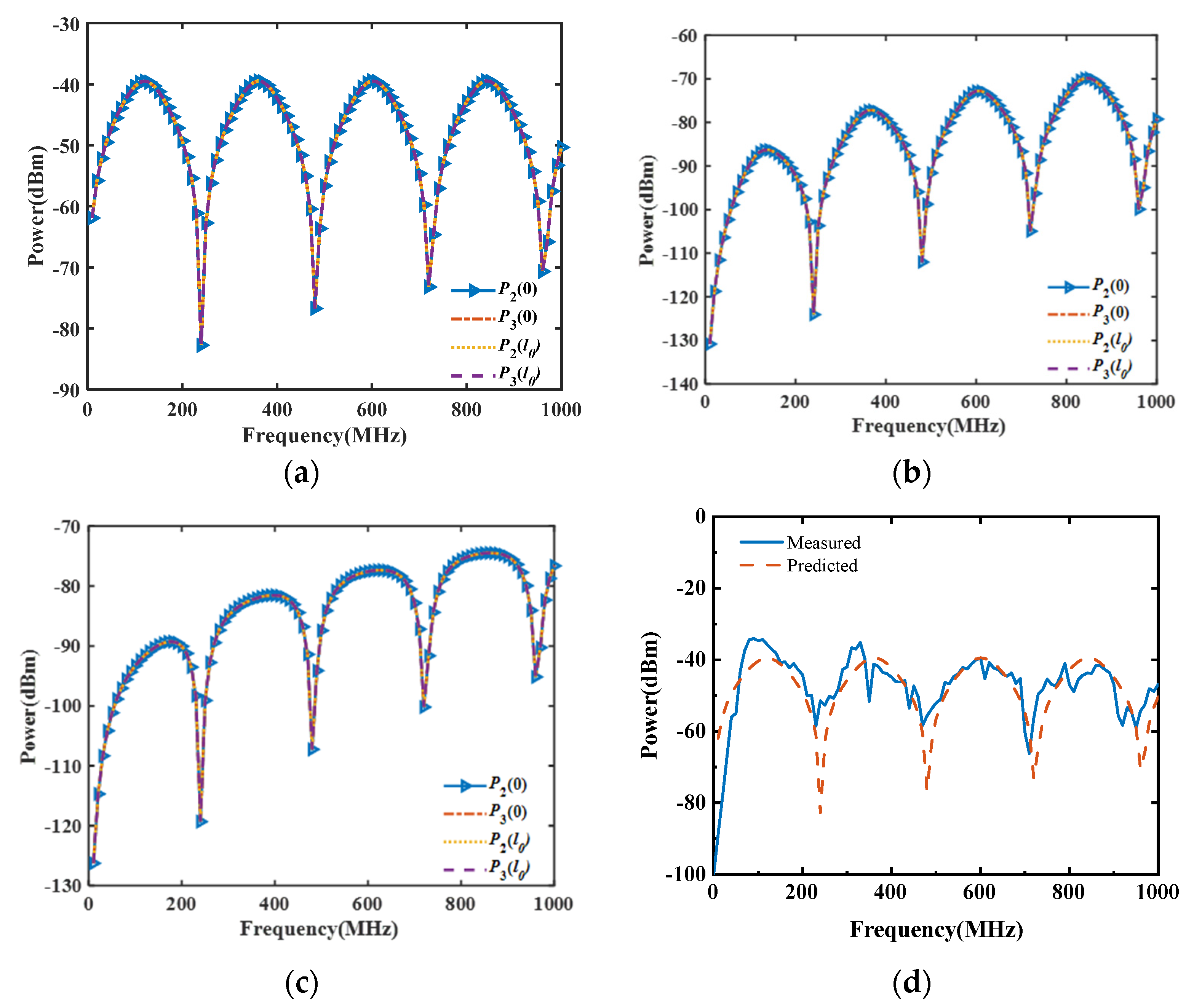
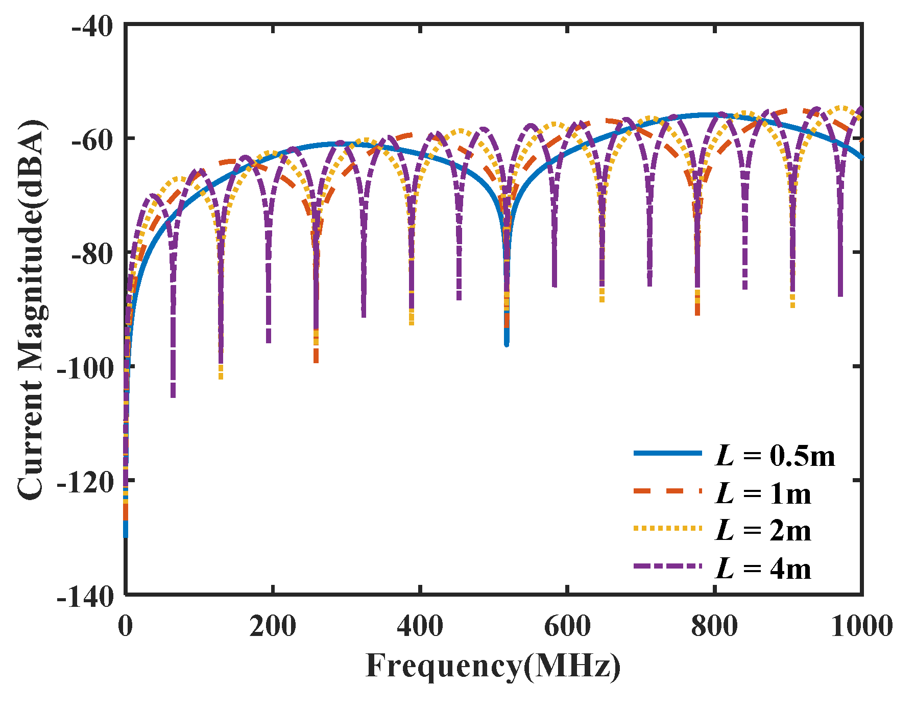
4.1. Effects of the Twisted Three-Wire Cable Length on Coupling Characteristics

The research object is a 24-AWG cable. The parameters of the twisted three-wire cable are as follows: pitch p = 0.1 m, separation distance 3 s , wire radius r = 0.25 mm, and s = 1.28 mm. Assuming that the outer dielectric of the wire is all lossless, as shown in Figure 4, when the frequency is higher than 1 MHz, the characteristic impedance of the twisted three-wire cable can be considered a real number. Therefore, the terminal impedance Z S and Z L are both set to 135 Ω.
Three different cases of plane-wave field excitation are defined. The electric field amplitude E = 2 V/m is set. In the first case, the plane wave is incident from the θ P = π / 2 and ϕ P = 0 direction, and the electric field polarization angle is provided by θ E = 0 . In this case, the wave propagates in the -y direction with the electric field polarized in the +z direction, which is referred to as perpendicular excitation (parallel). In this case of incidence and polarization, the electric field component is e x = 0 , e y =   0 , e z =   1 and the phase constant component is k x = 0 , k y = k , k z = 0 .
In the second case, the plane wave is incident from the θ P = π / 2 and ϕ P = 0 direction, and the electric field polarization angle is provided by θ E = π / 2 . In this case, the wave propagates in the −y direction with the electric field polarized in the +x direction, which is referred to as perpendicular excitation (vertical). In this case, the electric field component is e x = 1 , e y =   0 , e z = 0 , and the phase constant component is k x = 0 , k y = k , k z =   0 . In the above two cases, the electric field is parallel and perpendicular to the z-axis polarization direction, respectively.
In the third case, the plane wave is incident from the direction with θ P = π and ϕ P = 0 , and the electric field polarization angle is provided by θ E = 0 . In this case, the wave propagates in the +x direction with the electric field polarized in the -z direction, which is referred to as perpendicular excitation (vertical). In this case, the electric field component is e x = 0 , e y =   0 , e z =   1 , and the phase constant component is k x = k , k y =   0 , k z =   0 .
Using the above three different excitation methods, the currents at l = 0 and l = l 0 are calculated in combination with the twisted three-wire cable model. The results for these three excitation cases are shown in Figure 5.
In Figure 5, P 1 ( 0 ) and P 2 ( 0 ) are the current amplitudes for wire 1 and wire 2, respectively. P 1 ( l 0 ) and P 2 ( l 0 ) are the current amplitudes at l = l 0 for wire 1 and wire 2, respectively. The following results can be obtained by analyzing the above three excitation cases.
First, the polarization mode of the incident wave and the angle of incidence affect the current amplitude at the terminal of the twisted three-wire cable. As illustrated in (a) and (b) of Figure 6, a 90° change in the incident wave polarization causes a 22 dB change in the amplitude of the cable terminal coupling current. This demonstrates that the incident and polarization modes of the incident wave significantly affect the amplitude of the terminal coupling current.
Second, the twisted three-wire cable has frequency selective characteristics for electromagnetic irradiation response. The peak response of the terminal current is periodic.

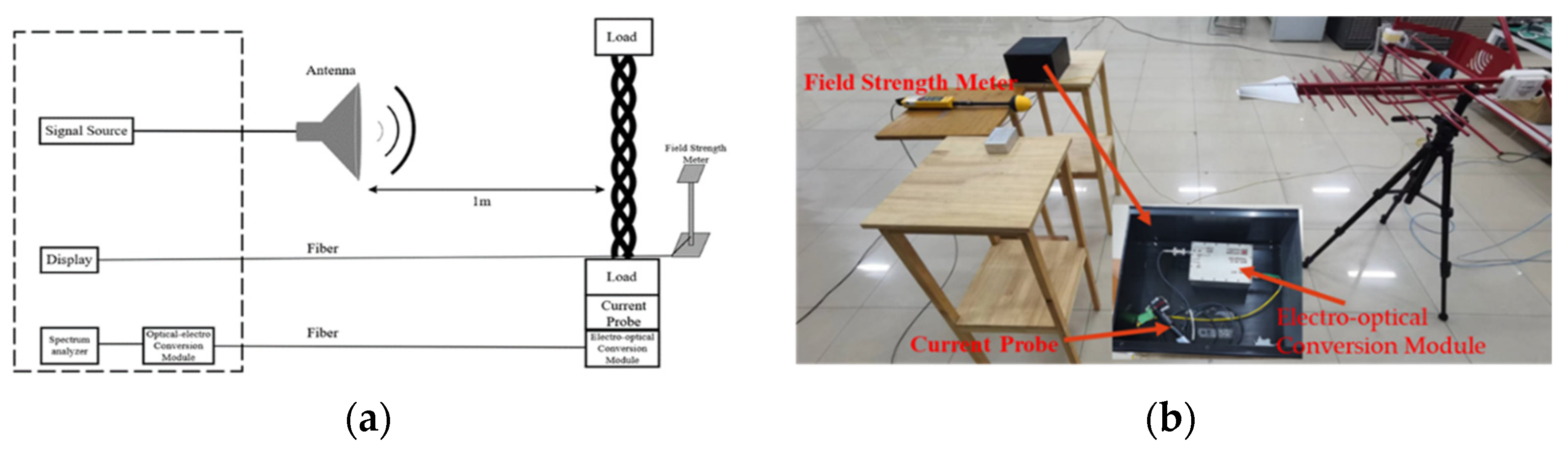
4.2. Experimental Validation

In order to validate the coupling response laws of the twisted three-wire cable under the plane wave electromagnetic irradiation conditions, a 1 m cable is tested, and the field strength of continuous wave is set to 2 V/m. The response signal is recorded by a spectrum analyzer. The configuration diagram of the irradiation test system is shown in Figure 6 and the experimental steps are as follows:
  • Cable Placement. A 1 m-long cable is placed on a horizontal table at a height of 1 m. The left and right ends are connected to a 50 Ω load resistance.
  • Field Strength Calibration. An antenna is positioned 1 m away from the twisted three-wire cable to serve as a radiation excitation source. The field strength is marked at 2 V/m.
  • System Setup: To monitor the load response at the right end, a single cable is passed through the current probe and then an optoelectronic conversion module is connected to the current probe at the right end of the load to convert the electrical signal of the load response into an optical signal. Another photoelectric conversion module is connected through optical fiber and connect it to the spectrum analyzer.
  • The values are recorded. Another irradiation test is conducted without changing the field strength and record the response on the cable within the desired frequency band.
Comparison of the measured result with the predicted result is shown in Figure 5d. Considering the simplicity of the transmission line model and the poor sensitivity of the test antenna and measurement equipment at low frequency, both the predicted and measured result are consistent for the excitation case in Figure 5a. This proves the reliability of the method and calculation results used in this paper.

5. The Twisted Three-Wire Cable Characteristics Discussion

5.1. Effects of the Twisted Three-Wire Cable Length on Coupling Characteristics

To investigate the roles of the length, the 24-AWG type cable is studied and terminated with a 135   Ω matched load by selecting a twisted three-wire cable with a pitch of 0.1 m and lengths of 0.5 m, 1 m, 2 m, and 4 m. As shown in Figure 7, we can obtain the following laws.
First, in the 0–1 GHz band, without changing the pitch, the increase in the total length of the cable does not cause a change in the peak current at the resonance point of the terminal coupling, i.e., the terminal response is not affected by the cable length. The peak coupling currents of the twisted three-wire cable at different lengths are connected into a constant envelope. The mean values of the peak currents at the resonance point for cables with total lengths of 0.5 m, 1 m, 2 m, and 4 m are −58.99 dBA, −59.12 dBA, −58.97 dBA, and −59.49 dBA, respectively.
Second, the number of resonance points increases with the increase in cable length in a fixed incident wave frequency band. In the 0–1 GHz band, the resonance points of the twisted three-wire cable with lengths of 0.5 m, 1 m, 2 m, and 4 m are 2, 4, 8, and 16, respectively. The distribution of resonance points in the peak current response band is related to the cable length.

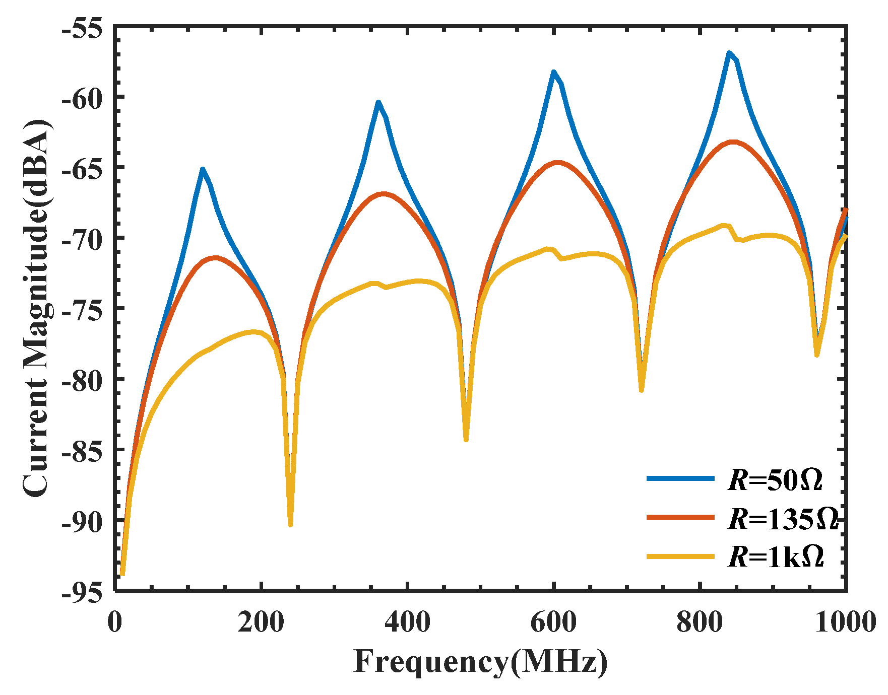
5.2. Effects of the Twisted Three-Wire Cable Termination Load on Coupling Characteristics

The changes in cable termination loads result in different termination responses in the same electromagnetic environment. Both ends of the cable are connected with the same resistance value, and the resistance value of the twisted three-wire cable terminal load is changed to set the resistance value for three cases of matched load R = 135 Ω, low impedance load R = 50 Ω, and high impedance load R = 1 kΩ. As shown in Figure 8, it can be observed that the variation of the terminal load under these three different load conditions does not change the distribution pattern of the cable resonance point, and the unmatched high impedance loads can reduce the current peak, which changes the response waveform of the cable terminal.

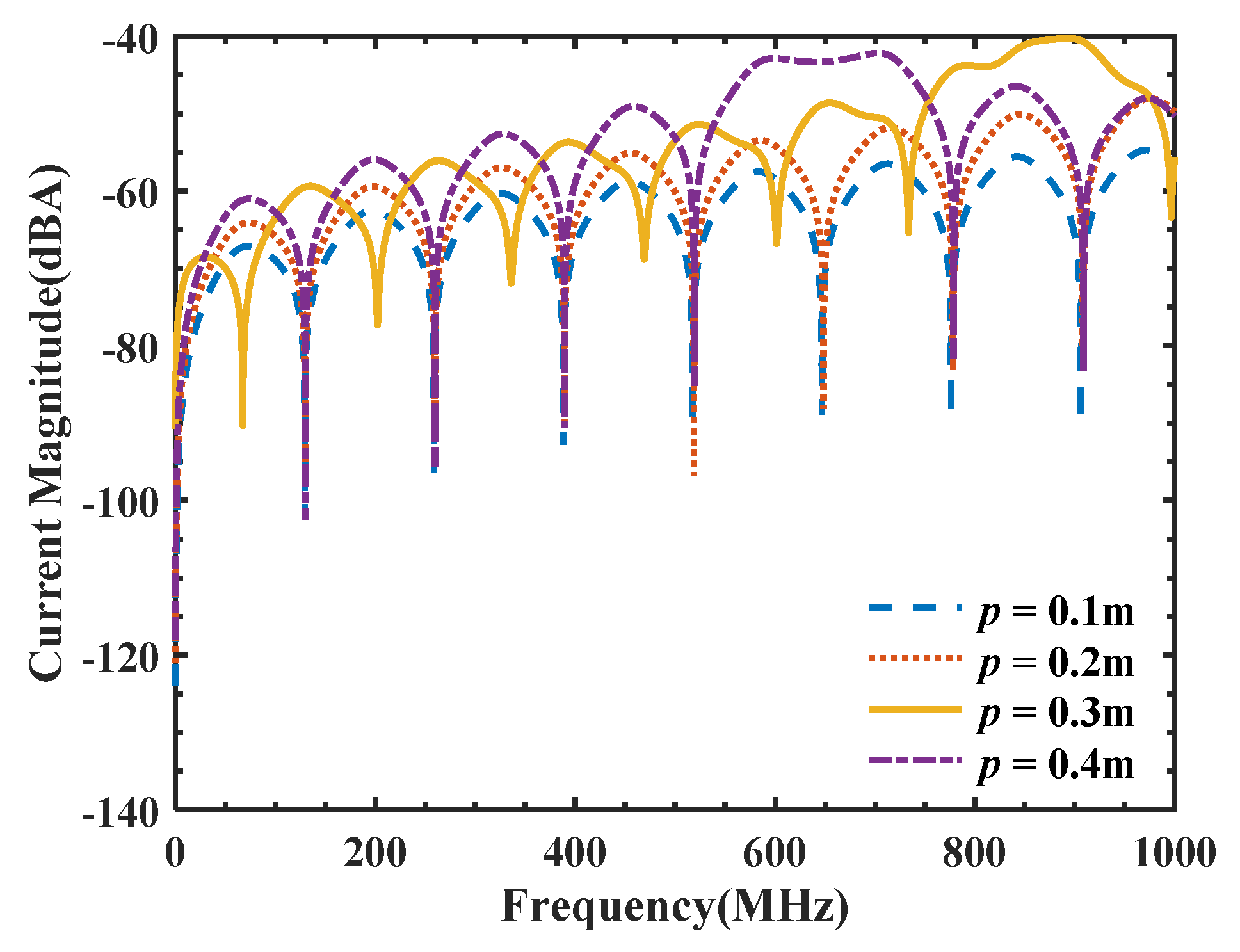
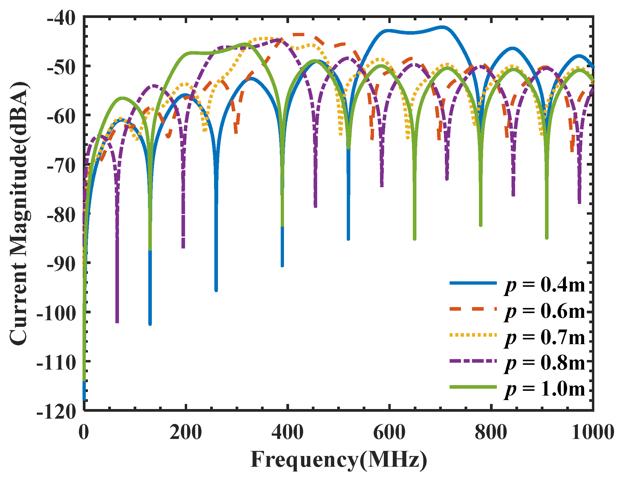
5.3. Effects of the Twisted Three-Wire Cable Pitch on Coupling Characteristics

In order to study the effect of pitch on the terminal response and coupling laws of the twisted three-wire cable, a cable with a length of 2 m is selected, and the pitches chosen are 0.1 m, 0.2 m, 0.3 m, and 0.4 m. The terminal response is shown in Figure 9. Therefore, we can obtain the laws described further.
First, under the condition that a line length is an integer number of spiral periods, changes in pitch do not affect the number and distribution pattern of resonant frequency points. As shown in Figure 9, the pitch is 0.1 m, 0.2 m, and 0.4 m, and the resonant frequency points are consistent when the integer number of twist periods is satisfied.
Second, the coupling energy increases with the increasing pitch for a given frequency band of the incident wave. As the pitch increases, the spiral coil area increases, which causes an increase in the magnetic flux incident into the spiral coil, thus increasing the energy coupling.
However, two problems cannot be ignored. When the pitch is 0.3 m, its resonant frequency point shifts. When the chosen pitch is 0.3 m, the spiral period is not an integer at this wire length, which destroys the resonance characteristics of the cable and makes it no longer have frequency selectivity.
Third, it is well known that imperfect twisting of the cable increases the value of crosstalk noise. As shown in Figure 9, the imperfect twisting portion of the cable changes the resonant characteristics of the twisted three-wire cable under external electromagnetic field irradiation. However, the current values of the cable coupling, in this case, remain essentially the same as those of the perfect twisting cable coupling. Therefore, we discuss such imperfect twisting cases.
In order to investigate the effect of length variation of imperfect twisting at different pitches, the cases of p = 0.4 m and p = 1 m are chosen as references, and three cases of imperfect twisting with pitches of 0.6 m, 0.7 m, and 0.8 m are selected. As shown in Figure 10, the resonance laws of the last integer number of twist periods are maintained for the cases of p = 0.4 m. The current amplitude in the case of pitch p = 0.4 m is higher than that in the case of p = 1 m. When the pitch is 0.6 m, 0.7 m, and 0.8 m, compared with the integer number of pitches, it is obvious that the resonance law of this cable has been destroyed. However, the coupling current values are all below the upper limit of current values for an integer number of twist periods. integer number of spiral periods

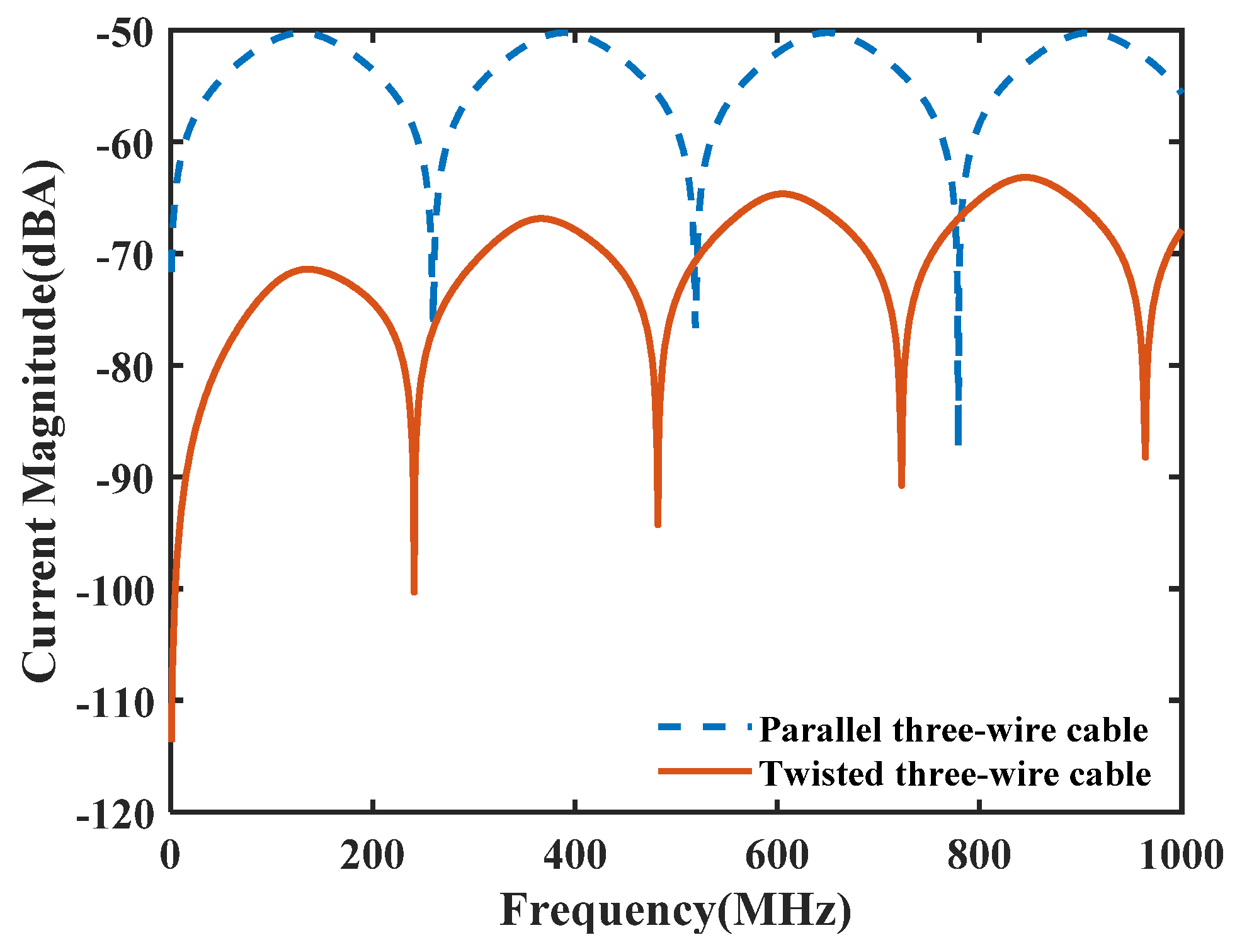
5.4. Response Comparison between the Twisted Three-Wire Cable and Parallel Three-Wire

The twisted three-wire and parallel three-wire 24-AWG cables were selected for comparison to explore the interference immunity characteristics of the stranded cable. Other parameters are set as follows: the incident plane wave θ P = π / 2 , ϕ P = 0 , θ E = π / 2 , and the structural parameters of the triple stranded wire are shown in Figure 4, and the structural parameters of the parallel three-wire cable are taken as l = 1 m, d = 2.56 mm.
Two observations can be drawn from Figure 11. One is that the triple-stranded structure does not change the frequency selection characteristics of the cable, and its frequency response laws are consistent with the parallel three-wire cable. The other is that compared with the coupling current results of the twisted three-wire cable and parallel three-wire cable, it can be determined that the coupling current of the twisted three-wire cable is 20 dB lower than the coupling current on the ordinary parallel three-wire cable. Therefore, the twisted three-wire cable has better anti-interference characteristics.

6. Conclusions

In this paper, a coupling model of the twisted three-wire cable under external planar electromagnetic wave irradiation is established, and the influence of parameters on the terminal response characteristics is investigated. The triple helix equations are introduced into the transmission-line-based theoretical field-to-wire coupling model. The terminal solution equations under plane wave irradiation are derived and extended to scenarios with arbitrary polarization and incident-direction wave irradiation. Then, the coupling characteristics of the twisted three-wire cable are obtained by changing the wire length, pitch, and termination load parameters of the cable and compared with the response of a parallel three-wire cable.
We obtain the following results: the twisted three-wire cable has a frequency selectivity characteristic for electromagnetic irradiation response, i.e., a periodic peak response occurs at fixed frequency intervals in a fixed incident wave band, and the number of resonant points increases with length. The increase in the total length of the cable affects the resonant frequency without increasing the value of the terminal response. Under the premise that the cable length and frequency band are certain, the coupling energy increases with the pitch increase, and the pitch change does not affect the number of resonant frequency points and the distribution pattern. Changes in the terminal load resistance of the twisted three-wire cable cannot change the frequency selectivity characteristic of the cable but influence the value of its terminal response. The twisted three-wire cable has good anti-interference characteristics compared to a parallel three-wire cable. The terminal response is reduced by about 20 dB under the same experimental conditions.

Author Contributions

Y.N. conceived of the study, designed the study, and wrote the manuscript. Y.C. and X.Z. provides guidance on ideas and mathematical treatment. M.Z. compiled the experimental data. Y.W. assisted in the editing of manuscripts. All authors have read and agreed to the published version of the manuscript.

Funding

This study did not receive any funding.

Data Availability Statement

The authors confirm that the data supporting the findings of this study are available within the article.

Conflicts of Interest

The authors declare that they have no conflict of interest regarding the publication of this paper.

References

  1. Zhou, L.; Zhang, S.; Yin, W.-Y.; Mao, J.-F. Immunity Analysis and Experimental Investigation of a Low-Noise Amplifier Using a Transient Voltage Suppressor Diode under Direct Current Injection of HPM Pulses. IEEE Trans. Electromagn. Compat. 2014, 56, 1715–1718. [Google Scholar] [CrossRef]
  2. Zhang, D.; Zhou, X.; Cheng, E.; Wan, H.; Chen, Y. Investigation on Effects of HPM Pulse on UAV’s Datalink. IEEE Trans. Electromagn. Compat. 2020, 62, 829–839. [Google Scholar] [CrossRef]
  3. van Leersum, B.; van der Ven, J.-K.; Bergsma, H.; Buesink, F.; Leferink, F. Protection Against Common Mode Currents on Cables Exposed to HIRF or NEMP. IEEE Trans. Electromagn. Compat. 2016, 58, 1297–1305. [Google Scholar] [CrossRef]
  4. Huangfu, Y.; Wang, S.; Di Rienzo, L.; Zhu, J. Radiated EMI Modeling and Performance Analysis of a PWM PMSM Drive System Based on Field-Circuit Coupled FEM. IEEE Trans. Magn. 2017, 53, 8208804. [Google Scholar] [CrossRef]
  5. Taylor, C.D.; Castillo, J.P. On the Response of a Terminated Twisted-Wire Cable Excited by a Plane-Wave Electromagnetic Field. IEEE Trans. Electromagn. Compat. 1980, EMC-22, 16–19. [Google Scholar] [CrossRef]
  6. Armenta, R.B.; Sarris, C.D. Efficient Evaluation of the Terminal Response of a Twisted-Wire Pair Excited by a Plane-Wave Electromagnetic Field. IEEE Trans. Electromagn. Compat. 2007, 49, 698–707. [Google Scholar] [CrossRef]
  7. Armenta, R.B.; Sarris, C.D. Modeling the Terminal Response of a Bundle of Twisted-Wire Pairs Excited by a Plane Wave. IEEE Trans. Electromagn. Compat. 2007, 49, 901–913. [Google Scholar] [CrossRef]
  8. Pignari, S.A.; Spadacini, G. Influence of twist-pitch random non-uniformity on the radiated immunity of twisted-wire pairs. In Proceedings of the 2011 XXXth URSI General Assembly and Scientific Symposium, Istanbul, Turkey, 13–20 August 2011; pp. 1–4. [Google Scholar] [CrossRef]
  9. Pignari, S.A.; Spadacini, G. Plane-Wave Coupling to a Twisted-Wire Pair Above Ground. IEEE Trans. Electromagn. Compat. 2011, 53, 508–523. [Google Scholar] [CrossRef]
  10. Spadacini, G.; Pignari, S.A. Numerical Assessment of Radiated Susceptibility of Twisted-Wire Pairs with Random Nonuniform Twisting. IEEE Trans. Electromagn. Compat. 2013, 55, 956–964. [Google Scholar] [CrossRef]
  11. Yuan, K.; Wang, J.; Xie, H.; Fan, R. SPICE Model of a Single Twisted-Wire Pair Illuminated by a Plane Wave in Free Space. IEEE Trans. Electromagn. Compat. 2015, 57, 574–583. [Google Scholar] [CrossRef]
  12. Yuan, K.; Wang, J.; Xie, H.; Fan, R. A Time-Domain Macromodel Based on the Frequency-Domain Moment Method for the Field-to-Wire Coupling. IEEE Trans. Electromagn. Compat. 2016, 58, 868–876. [Google Scholar] [CrossRef]
  13. Yuan, K.; Grassi, F.; Spadacini, G.; Pignari, S.A. Accounting for Wire Coating in the Modeling of Field Coupling to Twisted-Wire Pairs. IEEE Trans. Electromagn. Compat. 2018, 60, 284–287. [Google Scholar] [CrossRef]
  14. Gassab, O.; Yin, W.-Y. Characterization of Electromagnetic Wave Coupling with a Twisted Bundle of Twisted Wire Pairs (TBTWPs) above a Ground Plane. IEEE Trans. Electromagn. Compat. 2019, 61, 251–260. [Google Scholar] [CrossRef]
  15. Gassab, O.; Zhan, Q.; Zhou, L.; Yin, W.-Y. Transmission Line Model for a Shielded TWP with Apertures and Generalization to Braided–Shielded TWP Cables. IEEE Trans. Electromagn. Compat. 2021, 63, 2115–2123. [Google Scholar] [CrossRef]
  16. Zhao, M.; Chen, Y.; Zhou, X.; Zhang, D.; Nie, Y. Investigation on Falling and Damage Mechanisms of UAV Illuminated by HPM Pulses. IEEE Trans. Electromagn. Compat. 2022, 64, 1412–1422. [Google Scholar] [CrossRef]
  17. Paul, C.R. Analysis of Multiconductor Transmission Lines. Available online: http://www.researchgate.net/publication/241130019_Analysis_of_Multiconductor_Transmission_Lines (accessed on 6 October 2021).
Figure 1. Definition of starting coordinates of the twisted three-wire cable. Wire 1 is the reference wire, and both wire 2 and wire 3 are at a separation distance 3 s . t 12 ( l ) and t 13 ( l ) are the unit vectors of wire 2 and wire 3 pointing to wire 1.
Electronics 12 02018 g001
Figure 2. Definition of unit vector of the twisted three-wire cable. The geometric characteristics of the pair are cable pitch p, wire arc length l, and periodic structure.
Electronics 12 02018 g002
Figure 3. The parameters of the twisted line when radiated by the incident field of the uniform plane wave.
Electronics 12 02018 g003
Figure 4. The real part and imaginary part of the characteristic impedance of the 1 m−long 24−AWG twisted three-wire cable.
Electronics 12 02018 g004
Figure 5. Terminal responses of the twisted three−wire cable under three different planar wavefield excitations at the 135 Ω terminal impedances at l = 0 and l = l 0 in FD form. (a) Broadside with parallel polarization, (b) broadside with perpendicular polarization, (c) endfire, (d) comparison of measured result and predicted result.
Electronics 12 02018 g005
Figure 6. Irradiation test system configuration diagram. (a) System configuration diagram; (b) Physical connection of the system.
Electronics 12 02018 g006
Figure 7. Coupling characteristics of the twisted three−wire cable for different lengths when L = 0.5   m ,   1   m ,   2   m ,   4   m , r = 0.25   mm , p = 0.1   m , θ P = π / 2 , ϕ P = 0 , θ E = 0 , Z S = Z L = 135   Ω .
Electronics 12 02018 g007
Figure 8. Coupling characteristics of the twisted three−wire cable for different termination loads when L = 1   m , r = 0.25   mm , p = 0.1   m , θ P = π / 2 , ϕ P = 0 , θ E = 0 , Z S = Z L = 50   Ω ,   135   Ω ,   1   k Ω .
Electronics 12 02018 g008
Figure 9. Coupling characteristics of the twisted three−wire cable for different pitches when p = 0.1   m ,   0 . 2   m ,   0 . 3   m ,   0 . 4   m , L = 2   m , r = 0.25   mm , θ P = π / 2 , ϕ P = 0 , θ E = 0 , Z S = Z L = 135   Ω .
Electronics 12 02018 g009
Figure 10. Coupling characteristics of the twisted three−wire cable under imperfect twisting when p = 0.4   m ,   0 . 6   m ,   0 . 7   m ,   0 . 8   m ,   1   m , L = 2   m , r = 0.25   mm , θ P = π / 2 , ϕ P = 0 , θ E = 0 , Z S = Z L = 135   Ω .
Electronics 12 02018 g010
Figure 11. Comparison of current at l = 0 for parallel three−conductor cable and twisted three-wire cable when L = 1   m , r = 0.25   mm , p = 0.1   m , θ P = π / 2 , ϕ P = 0 , θ E = π / 2 , Z S = Z L = 135   Ω .
Electronics 12 02018 g011
Disclaimer/Publisher’s Note: The statements, opinions and data contained in all publications are solely those of the individual author(s) and contributor(s) and not of MDPI and/or the editor(s). MDPI and/or the editor(s) disclaim responsibility for any injury to people or property resulting from any ideas, methods, instructions or products referred to in the content.

