Abstract
This paper aims to solve the problem of the robust model predictive control, the contradiction of the system robustness, and the conservative terminal constraint set range. A robust model predictive control (RMPC) method based on an ε-approximation single-tube set is proposed. We construct a single-tube RMPC structure for linear discrete time invariant systems with additive disturbances. To this structure, we add the state estimation and state feedback to improve the convergence rate. Furthermore, we use the ε-approximation to estimate the terminal constraint set with less conservatism, thus improving the robustness. Then, we conduct a stability analysis of the ε-approximation single-tube RMPC system. The simulation results demonstrate the stability and interference allowance advantages of the proposed method.
1. Introduction
Model predictive control (MPC) is an efficient method, which is used in linear time-invariant systems [1,2,3,4,5]. The MPC leverages the model information to solve the optimal control problem by repeatedly minimizing the cost function, thus enabling favorable tracking effects and dynamic responses. However, the actual working conditions are complex, and the uncertain interference could reduce the system control precision. In this regard, many scholars have studied robust MPC.
In robust MPC (RMPC), state control and state constraints are restricted to ensure the system’s convergence and robustness [6,7,8,9,10,11]. In the RMPC research field, enhancing system robustness is a popular topic. It can be broadly categorized into two aspects, min–max RMPC and tube RMPC. Min–max RMPC method designs controllers by considering the worst disturbances [12,13,14,15,16,17]. The tube RMPC method computes a tube constraint set, where the constraint set is centered on the nominal predicted trajectory. Constraint sets are used to constrain the actual trajectory and thus minimize the error between the actual trajectory and the nominal predicted trajectory [18,19,20,21,22,23,24,25]. A numerically efficient linear matrix inequalities (LMls) method for calculating tightened invariant tubes was given by Cheng et al. [26], and simultaneously, the convergence range was reduced by the tightened tube constraint sets. Ping et al. [27] used time-varying scaled terminal constraint sets in an online tube-based RMPC optimization problem, which improved its flexibility. Sumeet et al. [28] designed a quasi-convex optimization program to compute a control contraction metric, which minimized the sizes of tube sets. Ping et al. [29] investigated a zonotopic set-membership state estimation method to reduce the conservatism of the tube constraint set and the online computational burden. Hu et al. [30] introduced a weighting factor to design a robust invariant set as a terminal constraint set, thus expanding the domain of the nominal control value.
Current research has identified several advantages of tube RMPC, such as the simplicity of the concept, the relatively little online computation, and the ease of application. As the tube constraint set has considerable influence on the robustness, some studies have been conducted to reduce the conservatism of the tube constraint set by expanding the range of the tube constraint set, so as to improve the system interference allowance. However, such changes increase the convergence range of the system and reduce its robustness. In addition, reducing the constraint set enhances the convergence of the system and also decreases the allowable range of the system disturbance, which limits the system’s ability to suppress a disturbance. Therefore, how to expand the interference allowance while efficiently suppressing the disturbance remains worthy of study in tube RMPC.
In this paper, we propose a single-tube RMPC method based on ε-approximation. The state estimation and feedback in a single-tube RMPC structure is designed to improve the response speed and convergence speed. The single-tube set is approximated by the ε-approximation, thus reducing the conservatism in the terminal constraint set and enhancing the system’s robustness. This method has several advantages, which make it an effective control method for linear discrete time invariant systems with additive perturbations. Applications of this method can be included in various fields, such as manipulator control systems, servo-motor control systems, and avionics and aerospace control systems.
This paper is organized as follows. The ε-approximation single-tube RMPC structure is established in Section 2. In Section 3, the ε-approximation of the single-tube terminal constraint set is proposed. Section 4 demonstrates the stability analysis of the ε-approximation single-tube RMPC. Section 5 gives the simulations of robustness to validate the effectiveness of the proposed method. Section 6 concludes this paper.
2. Single-Tube RMPC Structure
To investigate the robustness of a system under disturbance, in this paper, we study a constrained linear system with additive bounded disturbances. The structure of the single-tube RMPC structure is shown in Figure 1.
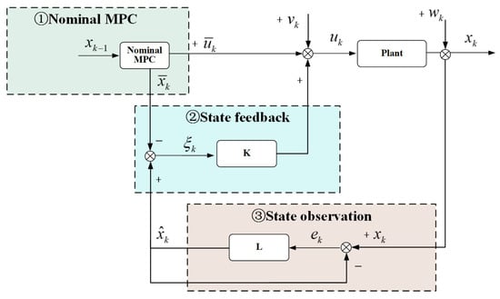
Figure 1.
Single-tube RMPC structure.
A single-tube RMPC structure comprises three parts: the nominal MPC, the error state estimation, and the error state feedback. represents the system state, is the system input, is the actual system output, is the system state disturbance, and is the system internal disturbance.
, , , and are constrained by Equation (2). Let , , , and represent the polyhedral sets, which contain the origin.
By neglecting the disturbances w and v, the consequential nominal MPC system can be given by Equation (3). and are the nominal MPC system state quantity and nominal MPC quantity, respectively.
We can obtain from the optimization problem in Equation (4).
Here, , the integer N is the prediction length, is the nominal MPC system state at the current time, is the nominal MPC reachable set, and R and Q are the weight matrices. is the optimal target state trajectory at prediction time k = [0, … k], and is the optimal control law. Thus, is the control law of the nominal MPC system at time k.
The feedback control in Equation (5) is included to eliminate the errors between the state observation and the actual system state. The parameter setting of the feedback matrix K should satisfy the condition wherein the spectral radius of is less than 1.
Due to the uncertain additive perturbations, the prediction accuracy is affected. The observation matrix L is presented to obtain the system estimated state.
is the estimated state, and L is the measurement matrix. The parameters of the observation matrix satisfy the condition wherein the matrix’s spectral radius is less than 1. The estimate error is defined as the error between the actual state and the estimated state . The prediction error is defined as the error between the nominal MPC state and the estimated state .
The actual state of the system is obtained by combining the above two systematic errors.
The single-tube error system is established by considering the estimated error and predicted error .
The constraint set is the robust invariant set of the single-tube error system state, and its terminal constraint set is the minimal robust invariant set. The computed symbol between the constraint sets represents the Minkowski sum, which is defined by adding the elements of sets A and B, . Equation (14) is used to obtain the constraint set of the actual error.
By combining Equations (12) and (13), the constraint set of the estimation error is obtained.
Let , be compact convex sets that satisfy , respectively, where and satisfy and , respectively, and satisfy monotonicity. Combining the method from [31] and the cumulative iteration of Equations (14) and (15), the minimal robust invariant sets , can be acquired.
When and are satisfied, and ; then, and will converge to and , respectively.
The minimal robust invariant sets and are used as the terminal constraint sets of the state errors and , respectively. However, the terminal constraint sets and need to be computed twice and have relatively small ranges; so, the interference allowance of the system is limited. Therefore, a method for an ε-approximation single-tube set computation is proposed in the next section to optimize the terminal constraint set calculation method.
3. ε-Approximation of the Single-Tube Terminal Constraint Set
In order to reduce the constraint set’s conservatism, and are treated as an overall state in this section. The constraint sets and are combined as one constraint set . The terminal constraint set only needs to be computed once, thus simplifying the computation.
3.1. Computation of the Single-Tube Terminal Constraint Set
We define the single-tube constraint variable as . Combining Equations (14)–(17) yields the single-tube constraint reduction process.
3.2. ε-Approximation of the Minimal Robust Invariant Set
The ε-approximation of the minimal robust invariant set is carried out, which expands the single-tube terminal constraint set range and reduces its conservatism.
ε-approximation [32]: When scalar ε > 0, there exists a set that is an ε-approximation of . There exists , where is computed in the form .
For any positive integer s, we define the constraint set as follows:
Each is contained in , until , . For every ε > 0, there exists a positive integer s, such that is an ε-approximation of . The computation of the single-tube constraint set is shown by the following formula.
We define α as a scalar, . , . If is a nilpotent matrix under the action of the exponent s, then can be approximated by . If is strictly stable but not a nilpotent matrix, an auxiliary equation is used to compute the ε-approximation of the minimal robust invariant set .
ε-approximation of the minimal robust invariant set: When exists, a finite positive integer s and a scalar satisfy condition , so that Equation (24) holds, , and .
Based on Equation (24), can approach through an effective relatively large s or relatively small α. For , , there exists an associated positive integer s satisfying the following relation.
Equation (25) shows that condition holds, thus realizing condition . Then, is an approximation of the minimal robust invariant set .
The auxiliary function is used to calculate the ε-approximation of .
The form of the auxiliary function is generalized to consider the set of state perturbation constraints as follows. , , and is a finite parameter.
The calculation of M(s) is as follows:
When is the jth standard basis vector, Equation (24) is equivalent to , when is valid.
The scalar α and scalar ε satisfy the following inequality.
Then, α is obtained by Equations (25)–(29). The ε-approximation of the minimal robust invariant set is obtained by Equation (24). Finally, is taken as an ε-approximation single-tube terminal constraint. Combining the above sections, the steps of the ε-approximation single-tube RMPC method are summarized in Table 1.

Table 1.
Steps of the ε-approximation single-tube RMPC method.
As shown in Table 1, steps 1–6 comprise the offline computations, and steps 7–9 comprise the online computations. As mentioned previously, for the single-tube terminal constraint set computed offline, the two computations are simplified to one, which reduces the computational pressure. The ε-approximation expands the original range of the terminal constraint set, thus improving the range of the interference allowance. Finally, the control state is stabilized in the terminal constraint set and converges to the origin. The proof of the control system stability analysis is given in the next section.
4. Stability Analysis of the ε-Approximation Single-Tube RMPC System
The proof of this process is divided into three steps. The stability of the system is analyzed by using the Lyapunov stability condition and two convergence conditions. First, we prove the recursive feasibility of the nominal model of the system. Then, we prove that the system error state converges to the ε-approximation single-tube terminal constraint set. Finally, we prove that the system error converges asymptotically to and near the origin within the terminal constraint set.
4.1. Recursive Feasibility of the Nominal MPC
Due to the nominal MPC, the quantity is equal to at time k and at time k + 1. We give the deviation calculation of the cost function at k + 1 and k.
Given the property and the finding that the nominal MPC ignores the uncertain disturbance, the following conclusions can be drawn by combining the above Equation (30).
Furthermore, the prediction solving inequality at time k + 1 is extended as follows:
In summary, we can conclude that is a bounded and nonincreasing sequence. The recursive feasibility of the nominal MPC is proved.
4.2. The System Error State Converges to the ε-Approximation Single-Tube Constraint Set
Satisfaction of robust constraints: As the nominal MPC recursion is feasible, and are satisfied at . and , are satisfied when is the system robust invariant set at . Then, and can be obtained by the constraint set reduction.
4.3. Recursive Feasibility of the Nominal MPC
Convergence: According to the recursively feasible nominal MPC, can be obtained from Equations (11) and (18). For , we can derive from ; for , is satisfied. Then, when , we can obtain and . Then, , and the system is asymptotically stable. In the case of interference, the system state gradually converges to the single-tube terminal constraint set and stabilizes to the origin and its vicinity.
By combining the above stability proofs, the system convergence process can be summarized as follows. First, the system error convergence trajectory is predicted by the nominal MPC. Then, the constraint set and terminal constraint set are computed offline. The system error is always contained in the in the terminal constraint set and continues to approach the predicted trajectory .
5. Simulation
To validate the advantages of the proposed method in disturbance suppression and fast convergence, a MATLAB simulation platform for the ε-approximation single-tube RMPC (STRMPC) and tube RMPC (TRMPC) methods was built, and the additive disturbance system described in [33] was taken as the controlled object. The controlled object was represented by the following linear time-invariant (LTI) system from Equation (1), where , , and .
The disturbance constraint , , , the state constraint , and the control constraint were satisfied, the weight matrix Q was [1,0; 0,1], and the weight matrix R was [0.01,0; 0,0.01]. The selected observation matrix parameter was L = [0.91, 0.75]. The feedback matrix parameter was K = [0.6136, 0.9962]. The predicted step size was N = 15.
In order to verify the advantages of the proposed method, the TRMPC was presented as a comparison. The nominal MPC part was the same as STRMPC, the feedback matrix parameter K, the predicted step size N, and the weight matrixes Q and R were also the same as the STRMPC. The differences in the control structure between the STRMPC and TRMPC are demonstrated below.
The TRMPC error state error was defined as , and the F matrix of the TRMPC was set as . The single-tube error system was set as . Combined with Equation (23), the terminal constraint set of the TRMPC was set as . Then, the terminal constraint set, single-tube error system state constraint set , and control value constraint set were used to calculate the nominal MPC reachable set. The comparison of the nominal MPC reachable sets and the terminal constraint sets are presented in Figure 2.
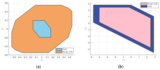
Figure 2.
Comparison of the terminal constraint sets and the nominal MPC reachable sets. (a) Terminal constraint sets. (b) Nominal MPC reachable sets.
As shown in Figure 2a, the ε-approximation single-tube terminal constraint set had a much wider range than the tube terminal constraint set. The wider range of the terminal constraint set reduced its conservatism and increased its interference allowance, thus increasing the system interference rejection capability and robustness. Due to the ε-approximation STRMPC and TRMPC using the same nominal MPC part, the nominal MPC reachable sets had almost same range as shown in Figure 2b.
5.1. Interference within the Constraint Range
The step response and sine wave tracing simulations are presented in this section. Step signals with a set value of 12 and sine wave signals with an amplitude of 12 and a period of 5 s were selected as the input signals. The TRMPC and STRMPC initial error state were set as .
- ①
- ±0.1 noise interference
The random white noise with an amplitude of ±0.1 was set as the state interference. The system error convergence comparison results and simulation output are shown in Figure 3 and Figure 4.
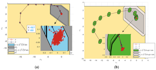
Figure 3.
Terminal constraint sets and state errors under ±0.1 noise interference. (a) Tube RMPC. (b) Single-tube RMPC.
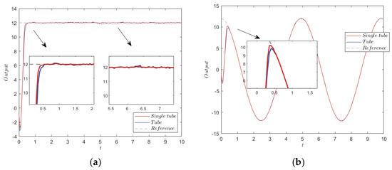
Figure 4.
Step response and sine wave tracking under ±0.1 noise interference. (a) Step response. (b) Sine wave tracking.
Figure 3a shows that the tube contained the nominal MPC state, the estimated system state, and the actual system state, which ensured the stability of the system. As shown by the convergence of the error states in Figure 3b, the actual system error states were contained in the single-tube terminal constraint set. The center of the set was the nominal MPC state, which was stabilized around the origin. Furthermore, the steady state error range of the TRMPC and STRMPC were both within ±0.1. The step response and sine wave tracking output comparison, in Figure 4, showed that the STRMPC had a more stable output and faster response speed.
- ②
- ±0.1 sine interference
The sine wave with an amplitude of ±0.1 was set as the state interference. The system error convergence comparison results are shown in Figure 5 and Figure 6. From Figure 5, the STRMPC and TRMPC converged the system state to the origin. Figure 6 presents the precision comparison of the sine wave tracking and the step response, and the simulation results showed that the ±0.1 sine interference could be effectively inhibited.
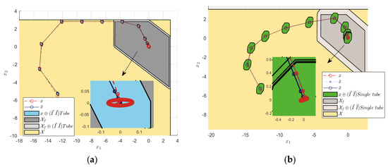
Figure 5.
Terminal constraint sets and state errors under ±0.1 sine interference. (a) Tube RMPC. (b) Single-tube RMPC.
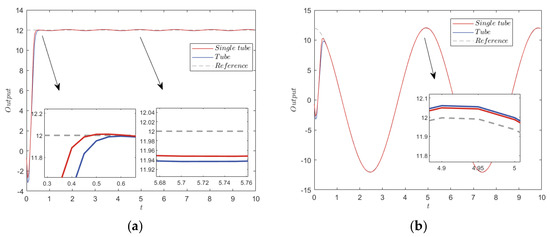
Figure 6.
Step response and sine wave tracking under ±0.1 sine interference. (a) Step response. (b) Sine wave tracking.
Combined with the above simulation results in Figure 3, Figure 4, Figure 5 and Figure 6, since there was no out-of-range interference in the system, we demonstrated that both the TRMPC method and the proposed method could suppress the noise and sine interference within the constraint range. According to Figure 4 and Figure 6, the proposed method had a better step response and sine wave tracking performance.
5.2. Interference Exceeding the Constraint Range
This part of simulation was designed to verify the advantages of the proposed method on suppressing interference, when the interference exceeded the constraint range. The random white noise interference and sine interference with ±0.5 amplitude were superimposed on the simulation output. We set the TRMPC and STRMPC initial error state . Step signals with a set value of 12 and sine wave signals with an amplitude of 12 and a period of 5 s were selected as the input signals.
- ①
- ±0.5 noise interference
The error convergence in Figure 7a shows that when the noise interference exceeded the disturbance constraint range, the actual state of TRMPC method exceeded the range of the terminal constraint set. However, Figure 7b shows that STRMPC can constraint the states within the terminal constraint set and stabilize states to near origin. In contrast to TRMPC method, STRMPC method can effectively suppress noise interference. The step response and sine wave tracking results in Figure 8 also demonstrate that STRMPC method can effectively suppress noise and have minor steady-state errors, when interference exceeding the constraint range.
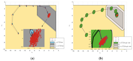
Figure 7.
Terminal constraint sets and state errors under ±0.5 noise interference. (a) Tube RMPC. (b) Single-tube RMPC.
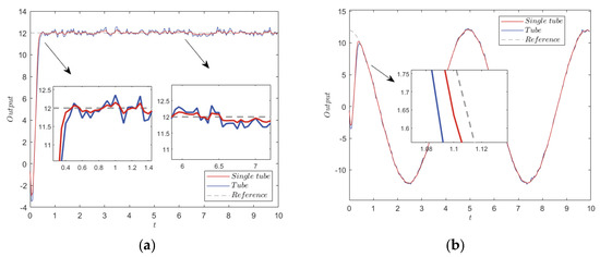
Figure 8.
Step response and sine wave tracking under ±0.5 noise interference. (a) Step response. (b) Sine wave tracking.
- ②
- ±0.5 sine interference
From Figure 9, for the state error convergence and the constraint set state, the STRMPC method had a more extensive terminal constraint set, and the allowable range of the sine interference was also expanded. In contrast, the TRMPC method had a conservative constraint set, and the system error state exceeded its terminal constraint set in the case of sine interference. Comparing the simulation results in Figure 10, the step response of the STRMPC was faster, and the steady-state error was smaller, which reached a steady state within a short period of time. The sine wave tracking result showed the tracking accuracy of the STRMPC.
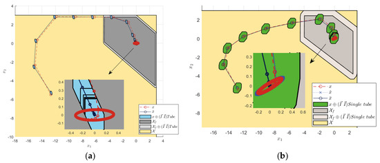
Figure 9.
Terminal constraint sets and state errors under ±0.5 sine interference. (a) Tube RMPC. (b) Single-tube RMPC.
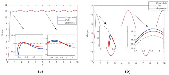
Figure 10.
Step response and sine wave tracking under ±0.5 sine interference. (a) Step response. (b) Sine wave tracking.
In order to further reflect the advantage of the proposed method on the disturbance rejection, we provided the integrated time absolute error (ITAE) criterion of the simulation results. The ITAE indexes of the STRMPC in Table 2 had smaller values than the TRMPC under different interference conditions. This implies that the proposed method had a faster convergence rate. The comparison of the ITAE indexes revealed that the ITAE index of the STRMPC method was less than that of the TRMPC method under the noise and sine interference, which exceeded the constraint range.
Table 2.
The ITAE index under the noise and sine interference.
The ITAE index reflects the response speed and stability of the system. In order to represent the stability and robustness of the system more comprehensively, the variances in the system error state and were calculated. Table 3 shows the proposed method had smaller variances than the TRMPC method, which means that the proposed method had a more stable output and less fluctuation.
Table 3.
Comparison of variances.
The above simulation results show that both the STRMPC and TRMPC methods suppressed the interference, when the noise and sine interference amplitudes were in the range of the pre-set interference. When the interference amplitude was extended, the TRMPC method could not suppress it because the set of terminal constraints was too small. In comparison, the STRMPC method has a wider set of terminal constraints, which improved the interference allowance and allowed the method to effectively suppress the interference.
5.3. Robustness Verification with Uncertain Model Parameters
A robustness verification simulation was carried out by floating the model parameters of the controlled plant by 10%. A noise interference of ±0.5 and sine interference of ±0.8 were further superimposed on the step response. The models with parameter fluctuations were set as f1, f2, f3, f4, and f5 in Table 4, where f3 was the original plant model. Step signals with a set value of 12 were selected as the input signal. The initial error state was .
Table 4.
Comparison of the model parameters.
The error convergence in Figure 11 shows that the systematic errors were slightly different in the initial case but eventually converged to the origin and remained within the constraint set, which verified the robustness of the STRMPC method. The simulation results in Figure 11, Figure 12 and Figure 13 show that the uncertainty of the model parameters had little influence on the step response; only the response velocities of the systems slightly deviated, and the steady state almost coincided. The noise and sine interference had little effect on the STRMPC system under model parameter uncertainty, and strong robustness was still ensured. In addition, the ITAE indexes in Table 5 and the variances in Table 6 had slight fluctuation, which further verified the robustness of the proposed method.
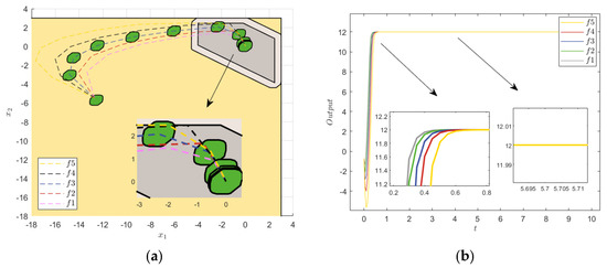
Figure 11.
Model parameter uncertainty. (a) Terminal constraint sets and state errors. (b) Step response.
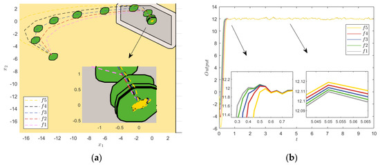
Figure 12.
Model parameter uncertainty and ±0.5 noise interference. (a) Terminal constraint sets and state errors. (b) Step response.
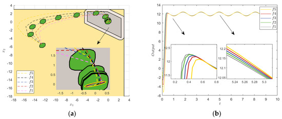
Figure 13.
Model parameter uncertainty and ±0.5 sine interference. (a) Terminal constraint sets and state errors. (b) Step response.
Table 5.
Comparison of the ITAE indexes.
Table 6.
Comparison of variances.
6. Conclusions
This paper proposes an ε-approximation single-tube RMPC method applicable to various linear discrete time invariant systems with additive disturbances, including manipulator control systems, servo-motor control systems, and avionics and aerospace control systems. Compared with the tube model predictive control, the proposed control method has a wider terminal constraint set and interference allowance, which is improved by ε-approximation. The system response speed is improved by single-tube state estimation and feedback. Moreover, the STRMPC has a better performance of interference rejection and a fast response. In particular, the robustness of the STRMPC was confirmed by simulations of model parameter uncertainties and interference within and exceeding the constraint range. We present the stability analysis of the ε-approximation single-tube error system. Simulations and theoretical analyses demonstrate that our proposed method is resistant to model parameter uncertainties, noise interference, and sine interference, especially when the interference exceeds the constraint range.
Author Contributions
S.L.: Methodology, Writing—original draft. B.X.: Writing—review and editing. C.W.: Project administration, Funding acquisition. L.W.: Visualization. Z.W.: Validation. X.L.: Supervision. All authors have read and agreed to the published version of the manuscript.
Funding
This research was funded by the Equipment Advance Research Field Foundation, grant number: 80923010202.
Data Availability Statement
Data underlying the results presented in the paper are not publicly available at this time but may be obtained from the authors upon reasonable request.
Conflicts of Interest
The authors declare that there are no conflicts of interests; we do not have any possible conflicts of interest.
References
- Clarke, D.W.; Mohtadi, C.; Tuffs, P.S. Generalized predictive control—Part I. The basic algorithm. Automatica 1987, 23, 137–148. [Google Scholar] [CrossRef]
- Mayne, D.Q.; Rawlings, J.B.; Rao, C.V.; Scokaert, P.O.M. Constrained model predictive control: Stability and optimality. Automatica 2000, 36, 789–814. [Google Scholar] [CrossRef]
- Maciejonski, J. Predictive Control with Constraints; Prentice-Hall: Hoboken, NJ, USA, 1999; ISBN 0-201-39823-0. [Google Scholar]
- Garcia, C.E.; Prett, D.M.; Morari, M. Model predictive control: Theory and practice—A survey. Automatica 1989, 25, 335–348. [Google Scholar] [CrossRef]
- Chen, H.; Allgöwer, F. A Quasi-Infinite Horizon Nonlinear Model Predictive Control Scheme with Guaranteed Stability. Automatica 1998, 34, 1205–1217. [Google Scholar] [CrossRef]
- Pin, G.; Raimondo, D.M.; Magni, L.; Parisini, T. Robust model predictive control of nonlinear systems with bounded and state-dependent uncertainties. IEEE Trans. Autom. Control 2009, 64, 1681–1687. [Google Scholar] [CrossRef]
- Limon, D.; Alamo, T.; Camacho, E.F. Input-to-state stable MPC for constrained discrete-time nonlinear systems with bounded additive uncertainties. In Proceedings of the IEEE Conference on Decision and Control, Las Vegas, NV, USA, 10–13 December 2002. [Google Scholar] [CrossRef]
- Pant, Y.V.; Abbas, H.; Mangharam, R. Robust model predictive control for non-linear systems with input and state constraints via feedback linearization. In Proceedings of the IEEE Conference on Decision & Control, Las Vegas, NV, USA, 12–14 December 2016; IEEE: Piscataway, NJ, USA, 2016. [Google Scholar] [CrossRef]
- Li, H.P.; Shi, Y. Robust distributed model predictive control of constrained continuous-time nonlinear systems: A robustness constraint approach. IEEE Trans. Autom. Control 2014, 59, 1673–1678. [Google Scholar] [CrossRef]
- Chisci, L.; Rossiter, J.A.; Zappa, G. Systems with persistent disturbances: Predictive control with restricted constraints. Automatica 2001, 37, 1019–1028. [Google Scholar] [CrossRef]
- Song, Y.; Wang, Z.D.; Wei, G.L. N-Step MPC for Systems With Persistent Bounded Disturbances Under SCP. IEEE Trans. Syst. Man Cybern. Syst. 2020, 50, 4762–4772. [Google Scholar] [CrossRef]
- Ping, X.; Yang, S.; Wang, P.; Li, Z. An observer-based output feedback robust MPC approach for constrained LPV systems with bounded disturbance and noise. Robust Nonlinear Control 2020, 30, 1512–1533. [Google Scholar] [CrossRef]
- Tang, X.; Deng, L. Multi-step output feedback predictive control for uncertain discrete-time T–S fuzzy system via event-triggered scheme. Automatica 2019, 107, 362–370. [Google Scholar] [CrossRef]
- Yang, W.; Gao, J.; Feng, G.; Zhang, T. An optimal approach to output–feedback robust model predictive control of LPV systems with disturbances. Robust Nonlinear Control 2016, 26, 3253–3273. [Google Scholar] [CrossRef]
- Ping, X.; Wang, P.; Zhang, J. A multi-step output feedback robust MPC approach for LPV systems with bounded parameter changes and Disturbance. Control Autom. Syst 2018, 16, 2157–2168. [Google Scholar] [CrossRef]
- Tang, X.; Deng, L.; Liu, N.; Yang, S.; Yu, J. Observer-based output feedback MPC for T–S fuzzy system with data loss and bounded disturbance. IEEE Trans. Cybern. 2019, 49, 2119–2132. [Google Scholar] [CrossRef] [PubMed]
- Li, D.; Xi, Y.; Gao, F. Synthesis of dynamic output feedback RMPC with saturated inputs. Automatica 2013, 49, 949–954. [Google Scholar] [CrossRef]
- Riverso, S.; Farina, M.; Ferrari-Trecate, G. Plug-and-play model predictive control based on robsut control invariant sets. Automatica 2014, 50, 2179–2186. [Google Scholar] [CrossRef]
- Riverso, S.; Ferrari-Trecate, G. Tube-based distributed control of linear constrained systems. Automatica 2012, 48, 2860–2865. [Google Scholar] [CrossRef]
- Cannon, M.; Kouvaritakis, B.; Rakovic, S.V.; Cheng, Q. Stochastic tubes in model predictive control with probabilistic constraints. IEEE Trans. Autom. Control 2011, 56, 194–200. [Google Scholar] [CrossRef]
- Mayne, D.Q.; Seron, M.M.; Rakovic, S.V. Robust model predictive control of constrained linear systems with bounded disturbances. Automatica 2005, 41, 219–224. [Google Scholar] [CrossRef]
- Cannon, M.; Buerger, J.; Kouvaritakis, B.; Rakovic, S. Robust tubes in nonlinear model predictive control. IEEE Trans. Autom. Control 2011, 56, 1942–1947. [Google Scholar] [CrossRef]
- Mayne, D.Q.; Kerrigan, E.C.; Wyk, E.J.; Falugi, P. Tube-based robust nonlinear model predictive control. Int. J. Robust Nonlinear Control 2011, 21, 1341–1353. [Google Scholar] [CrossRef]
- Sun, T.R.; Pan, Y.P.; Yu, H.Y. Robust model predictive control for constrained continuous-time nonlinear systems. Int. J. Control 2018, 91, 359–368. [Google Scholar] [CrossRef]
- Rakovic, S.V.; Kouvaritakis, B.; Findeisen, R.; Cannon, M. Homothetic tube model predictive control. Automatica 2012, 48, 1631–1638. [Google Scholar] [CrossRef]
- Hu, C.; Liu, C.; Jaimoukha, I.M. Computation of Invariant Tubes for Robust Output Feedback Model Predictive Control. IFAC-PapersOnLine 2020, 53, 7063–7069. [Google Scholar] [CrossRef]
- Ping, X.B.; Yao, J.Y.; Ding, B.C.; Li, Z. Tube-Based Output Feedback Robust MPC for LPV Systems With Scaled Terminal Constraint Sets. IEEE Trans. Cybern. 2022, 52, 7563–7576. [Google Scholar] [CrossRef] [PubMed]
- Sumeet, S.; Pavone, M.; Slotine, J.-J.E. Tube-Based MPC: A Contraction Theory Approach. In Mathematics, Engineering; Springer: Berlin/Heidelberg, Germany, 2016. [Google Scholar]
- Ping, X.; Yang, S.; Ding, B.; Raïssi, T.; Li, Z. Observer -based output feedback robust MPC via zonotopic set -membership state estimation for LPV systems with bounded disturbances and noises. J. Frankl. Inst.-Eng. Appl. Math. 2020, 357, 7368–7398. [Google Scholar] [CrossRef]
- Hu, C.F.; Wei, X.F.; Ren, Y.L. Passive Fault-tolerant Control Based on Weighted LPV Tube-MPC for Air-breathing Hypersonic Vehicles. Int. J. Control Autom. Syst. 2019, 17, 1957–1970. [Google Scholar] [CrossRef]
- Rakovi, S.V.; Kouramas, K.I.; Kerrigan, E.C.; Allwright, J.C.; Mayne, D.Q. The Minimal Robust Positively Invariant Set for Linear Difference Inclusions and its Robust Positively Invariant Approximations. Mathematics 2005, 50, 406–410. [Google Scholar]
- Rakovic, S.V.; Kerrigan, E.C.; Kouramas, K.I.; Mayne, D.Q. Invariant approximations of the minimal robust positively Invariant set. IEEE Trans. Autom. Control 2005, 50, 406–410. [Google Scholar] [CrossRef]
- Lorenzetti, J.; Pavone, M. A Simple and Efficient Tube-based Robust Output Feedback Model Predictive Control Scheme. In Proceedings of the European Control Conference, Saint Petersburg, Russia, 12–15 May 2020; IEEE: Piscataway, NJ, USA, 2020. [Google Scholar] [CrossRef]


Disclaimer/Publisher’s Note: The statements, opinions and data contained in all publications are solely those of the individual author(s) and contributor(s) and not of MDPI and/or the editor(s). MDPI and/or the editor(s) disclaim responsibility for any injury to people or property resulting from any ideas, methods, instructions or products referred to in the content. |
© 2023 by the authors. Licensee MDPI, Basel, Switzerland. This article is an open access article distributed under the terms and conditions of the Creative Commons Attribution (CC BY) license (https://creativecommons.org/licenses/by/4.0/).