Abstract
Technological advances in the internet of things (IoT) allowed a low-cost, yet small sensor device to operate with limited power in a dynamic harsh environment where human intervention is impossible. The wireless sensor network (WSN) is an example of the IoT in which physical devices’ software and sensors can interconnect to provide application services. It is important that such applications be dependable to meet the required quality of service (QoS) and function as expected. Consequently, the multi-objective optimization (MOO) problem in WSNs aims to address the trade-off among coverage, connectivity, and network lifetime requirements. Node scheduling is one approach of many used to optimize energy in WSNs. The contribution of this work is the proposal of a self-organizing feature map (SOFM) to enhance the node scheduling in WSNs. The proposed SOFM node-scheduling algorithm aims to spatially explore the state space domain and obtain an optimal solution. In our experiment, the proposed SOFM node-scheduling algorithm is evaluated against a comparable algorithm, namely the BAT node-scheduling algorithm, via MATLAB simulator. The results showed that the SOFM node-scheduling algorithm outperformed the latter by 27% and 28% for the maximum and minimum coverage, respectively, with similar performance of 99% of connectivity and network lifetime.
1. Introduction
A typical WSN is formulated out of multiple sensor nodes connected to each other through one or two base stations to provide application services [1,2]. The WSN applications can range from simple detection systems, i.e., environmental monitoring systems, to complex safety-critical systems, i.e., forced fire detection systems, as shown in Figure 1. Such safety-critical applications have real-time requirements which, in some cases, require an immediate alert response from the network [3]. For example, a forest fire detection system requires rapid detection of a fire breakout, so the incident can be mitigated as soon as possible without causing any casualties such as loss of forest, animals, and people in the forest. Another example is the use of the earthquake early warning system (EEWS), which requires instantaneous detection of the ground motion before, during, and after the earthquake [2,4,5]. Therefore, the specification requirements of a dependable WSN safety-critical system must be taken into consideration to ensure proper and functional operations.
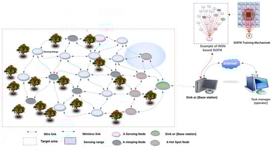
Figure 1.
The WSN architecture with the use of fire forest detection systems.
It is important that such safety-critical systems continuously and accurately provide the required parameter values, such as temperature, humidity, motion, and light, within the specified critical time constraint. Hence, the dependability of such a network must be as high as possible to ensure the optimal QoS requirements [6,7]. Meeting this time constraint and aligning with safety requirements and standards are crucial for real-time monitoring and decision making. According to European standardization, a WSN safety-critical system must have quick detection for such phenomena and report to the centers of authorities as quickly as possible within its occurrence [1,2]. The motivation of this paper is to enhance the dependability of safety-critical WSNs by exploring the state space and, in the process, finding the optimal solution [8]. Our hypothesis envisages best-connected coverage with the best meaningful and useful network lifetime solution. Subsequently, the WSN must operate correctly during the run time according to its specification requirements. Thereby, the main contribution of this paper is addressing the MOO problem and finding the balance among coverage, connectivity, and network lifetime. Thus, we propose a novel SOFM node-scheduling algorithm to maintain network dependability, viability, availability, and reliability. The novelty of our approach is in its application in the MOO problem domain which is an NP-hard problem [9,10]. Furthermore, the proposed solution provides an optimal network configuration based on the SOFM spatial representation model in the context of safety-critical WSNs.
In its most basic form, the SOFM model emerged from the standard self-organizing map (SOM) technique, which allows dimensionality reduction for the data in the state space from a higher dimensional space to a lower dimension space [11]. The SOM technique has a unique property of producing feature maps that can be visually observed and then identified. By proof, the feature map of surfaces tends to converge on global maxima and minima rather than local maxima and minima. In SOFM, nodes are programmed to learn and become their input values/parameters by mapping their weights to follow their given input data [12]. In order to understand the concept of the SOFM, first we must illustrate its basic framework. In principle, the SOFM is the process of randomly choosing a node from a map or a grid and comparing its distance with the distance of all other nodes in the grid [13]. There are many methods to calculate the distance between the nodes in the grid. The Euclidean distance is one method, and is the shortest line between two points A source and B destination, as shown in Figure 2.
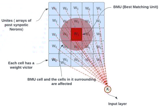
Figure 2.
Updating the best matching unit and its neighbors.
For example, in Figure 2 we assumed node Xi is randomly selected from the grid as a first node X1; then, the distance between X1 and the rest of the nodes in the grid is calculated, where the closest node to X1 is found and specified. The red dashed lines represent the association of this node (i.e., X1) with all the nodes in the grid, where each red dashed line has an associated weight value. Once the closest node is specified, it is then considered the best matching unit (BMU). Then we start updating the values of all the nodes in the grid according to the input, which is Xi, e.g., the BMU found. Note that we try to edit a certain range by a certain percentage. This update happens with different values but at a close range to the BMU (e.g., sensor node) that is initially found. The main goal of the SOFM is that the BMU value will reach the same absolute value as X1. This process is iterated from one node to another (X1, X2 …Xi), where another node in the grid, in this case X2, is chosen for the same calculation of applying the Euclidean distance and comparing and reapplying the same process [14].
In a typical SOFM, the optimization mechanism works towards decreasing the problem-to-solution domain from multiple dimensions (e.g., 23) to limited dimensions (e.g., 3), which makes it very easy to handle. It allows us to handle a large amount of data in manageable datasets without losing their functional properties with respect to the optimized solution. In this work, the main objective is to optimize the WSN to perform reliably for safety-critical applications. Hence, we propose the SOFM model by utilizing important features that are based on update functions, unlike the hidden markov model (HMM) and BAT node-scheduling algorithms which are based on activation functions.
Hence, this paper is organized as follows: in Section 2, we delve into the current state-of-the-art SOFM node-scheduling algorithms and their constraints. Section 3 outlines the problem formulation within the context of a WSN. Section 4 covers the simulation experiments and the resulting outcomes. In Section 5, the conclusion of the work is drawn.
2. Related Work
There is a plethora of work that addresses energy optimization in the WSN [15,16]. However, only a few works attempted to address energy optimization from the perspective of the MOO problem, which consider a suitable trade-off across the three dimensions: connectivity, coverage, and network lifetime. In what follows, we shed light on some of the most important ones in the literature that use the SOM model to address the problem of energy optimization in the WSN [16]. For example, the author in [17] utilized SOM to propose an energy optimization model to reduce communication in clustered WSNs. In particular, the author proposed an approach for cluster selection based on the extension to growing self-organizing map (E-GSOM) technique. The author compared two evolutionary-based genetic computing techniques against the E-GSOM, where the result showed an improvement in energy efficiency among its peers. The ref. [18] investigated the latest state-of-the-art approaches in low-cost fixed relay clustering problems in energy-harvesting wireless sensor networks (EHWSNs). The author proposed random relay fixed clustering for EHWSNs. The protocol divides the network into k number of ring areas of an equal width size, where each ring area is divided into the same number of CHs. This strategy introduced a metric for random selection of the CH as relay nodes. However, this study does not consider the energy consumption for the selection of the CH relay nodes.
Another interesting solution was provided by Xie et al. [19] for the connected coverage problem in WSNs. The authors proposed an active node communication strategy to provide a spatial optimal coverage solution for dynamic networks. In the proposed communication strategy, active nodes compensate for the coverage and connectivity that are introduced by the static nodes. Although this is an interesting solution to the dynamic nature of the WSN, it requires the use of mobility to compensate for the coverage and connectivity, which might be infeasible and inapplicable for other types of WSNs.
Another work that utilized SOFM to provide efficient cluster-routing algorithms was proposed by [17]. The work reduces energy consumption by organizing sensor nodes into clusters, whereby better communication nodes in the WSN are minimized. The solution improves the network lifetime via the distance reduction among CH nodes and load-balancing cost function. Since communication is the most expensive energy expenditure in a WSN, the proposed solution managed to optimize communication distance among CHs by reducing the communication distance to the base station. Although this approach extends the network lifetime by reducing the communication distance to the base station, the proposed approach incurs messages overhead due to the setup cost of forming the CHs with the short distinct to the base station.
On the other hand, the author in [20] introduced the self-organizing map scheduling algorithm (SOMSA) for sensor networks where the scheduling of the nodes is based on dynamic environment settings with local interactions. These settings are entirely based on the changing energy levels of the WSN. The SOM, therefore, uses these patterns as input vectors to produce dynamic scheduling for efficient data transfer. In our case, we already computed the final scheduling before the WSN operation. However, in the case of [20], the scheduling is dynamically computed using the SOFM; hence the energy consumption is more in this case than ours due to the message control exchange overhead.
In ref. [21], the author proposed the SOFM topology building (SOFMTB) algorithm to optimize energy in WSNs. The work utilized the SOFM technique to adjust the clusters based on energy levels for efficient dissemination of data over the network. The SOFMTB divides the WSN into tiers using the k-means algorithm as the cluster head and cluster members. It also modifies the topology of the network, providing efficient partitions in the network.
In ref. [13], SOFM was used to reduce energy consumption and bandwidth usage in a resource-constrained WSN. The solution tends to reduce the data communication during the entire network lifecycle by reducing its size. For instance, in this work, 1500 data volumes were generated and aggregated from all sensor nodes and sent to the base station. This approach clusters these data and reduces their size by selecting the most suitable size that has the meaningful one and sending it instead of that 1500 large-volume one.
On the other hand, the work in ref. [22] used the self-organizing map technique for high buildings, in the HVAC system, to find energy-saving opportunities and thus efficiently distribute the energy. This work used a dataset spanning one-year in time series analysis to provide a service that accommodates user requests regarding outdoor/indoor temperature. Utilizing SOM was proven to provide an energy-efficient solution.
In summary, having assessed the latest state-of-the-art node-scheduling techniques that utilize the SOM model in WSNs, it has been noticed that the existing literature lacks solutions that address the three requirements together, i.e., coverage, connectivity, and network lifetime, which are crucial for dependable a WSN. Hence, there is still more room to explore the state space to obtain the optimal solution with respect to the MOO, which is what motivated this work. Therefore, the SOFM node-scheduling algorithm is proposed to find the optimal scheduling for the MOO problem.
3. Problem Formulation
To explore the search space and find the optimal solution for the MOO problem, especially in the context of the WSN safety-critical systems, we used a multidisciplinary approach (i.e., that combines the optimization of three objectives: coverage, connectivity, and network lifetime) utilizing the SOFM model spatial feature to formulate and solve the MOO problem. Therefore, this work proposes a novel node-scheduling algorithm using the SOFM node-scheduling algorithm. In the SOFM node-scheduling algorithm, nodes are grouped according to their similar features. For example, in the WSN, nodes share similar features such as energy levels, transmission (Tx), receiving (Rx), and distance (D) from the sink node or distance between the parent to child nodes; the fifth feature is the sleep/awake scheduling. The main purpose is to reduce high-dimensional data to a map.
Henceforth, we assume a dataset of size (m, n), where m is the number of training examples, e.g., the number of sensors in the WSN, and n is the number of features; a matrix of (100, 2) initializes weights (n, C), where C is the number of clusters. Iterating over the input data for each training example, it updates the weight vector with the shortest distance (Euclidean distance) from the training example. The updated rule of weight is represented in Equation (3). The general structure of the SOFM node-scheduling algorithm is represented from [14], where we start the formulation by calculating the Euclidean distance (e.g., the shortest distance between two vectors) as in Equation (1):
where D is the Euclidean distance, x and y are the cartesian coordinates of the nodes in the field, where (x1, y1) and (x2, y2) are the input coordinates of the randomly selected vector/neuron. The mc is the Codebook (feature set) vector matching a given input vector X, as described in Equation (2):
mi is the average spatial x-coordinate of a neuron. In this work, we formally defined mc as the neuron (sensors).
The SOFM units receive updates, as well as their neighbors where the unit of the highest match is achieved. Within such a process, the best unit becomes updated closer to the sample vector in the space of the input value, as in Equation (3):
where alpha is a learning rate at time t, j denotes the winning vector, i denotes the feature of the training example, and k denotes the . training example from the input data. After training the SOFM network, the trained weights are used for clustering new examples. A new example falls in the cluster of winning vectors. The first step is to find the distance between two sensor nodes. For example, if the distance between, say, node A and node B is found, then they will be compared; at that point, the distance between sensor B and sensor C can also be found. The calculations for clustering new examples are performed using Equation (4):
where represents the Euclidean distance, which can be found in terms of the Euclidean norm of the difference between two vectors (sensor nodes). Please note that A and B represent two sensor nodes in the system, as shown in Equation (5):
Finally, the BMU is updated with respect to the next immediate neighbor, usually noted as , which is represented by Equation (6):
Equation (6) represents the normalization of the input vector X and the output vector, where the value of the output vector is equivalent to the minimum Euclidean distance between the normalized input vector and the path weight vector.
The purpose of Equation (6) is to identify the nodes which can be CH nodes, i.e., the nodes have better position and energy levels. For example, if three sensors are considered, A, B, and C, logically there will be a path from A to B and a path from B to C; hence, there are two paths having two distances that are denoted by D0 and D1. If D0 > D1, then the B sensor is not a CH; otherwise, it then becomes a CH. Operating the function in Equation (6) might find more CHs than required; hence, another function is needed that will select the best five CHs among them. The second function updates the weights and assigns each weight to the sensor node. This function will collect the highest weights assigned to the sensor nodes. Hence, the pseudocode of the SOFM node-scheduling algorithms is presented in Algorithm 1.
| Algorithm 1: SOFM node-scheduling algorithms | |
| Input: |
|
| Output: | SOFM Optimized 5 features for creating efficient network for WSN. |
| |
The operational setup of the SOFM algorithm includes the five features mentioned earlier; each feature is associated with a certain weight value, which needs to be updated in every iteration based on those features. Here the Euclidean distance is calculated and the best matching is identified where the clustering starts to form a group as a potential solution. Each group would have its own sleep scheduling, which is based on a value obtained from the features. All these processes are calculated by the sink node during the design time and implemented in the run time. Figure 3 illustrates the output of the SOFM node-scheduling algorithm to create an efficient network for the WSN.
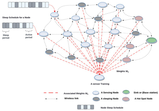
Figure 3.
The visualization of the WSN using the SOFM node-scheduling algorithm.
These features are fed into the SOFM model to provide the best node-scheduling process where the SOFM node-scheduling algorithm can be used to find the winner node consisting of the best of the available features amongst all other available nodes. The mechanism of the SOFM node-scheduling algorithm is based on the energy levels of the sensor node and the distances between the CH and sink, parent, and child nodes, Tx, Rx, and the node sleep/awake scheduling. Thus, the SOFM node-scheduling algorithm partitions the network in the form of five-dimensional space layers.
In order to illustrate the principle of the five-dimensional space layers, let us consider a simple example of three layers starting from one to three, where layer one is presented for the information dissemination, e.g., packet exchanging. As the WSN progresses in time, after SOFM node-scheduling algorithm iterations, some sensor nodes will experience a change in the level of energy, i.e., consume energy. Those sensor nodes are then replaced with other nearby available nodes that have the same features from the next layers, e.g., updated from layer two and consequently layer three. After some time, the layer under consideration will exhaust the solutions; now the onus is on the immediate next layer to take on the responsibility of the presently running node.
4. Results and Discussion
The simulation experiment was conducted using a MATLAB_R2018b environment. In this experiment, we compare the new proposed SOFM node-scheduling algorithm against the BAT node-scheduling algorithm, hence spatially exploring the state space of the problem domain. The considered assumptions are as follows:
- The WSN-monitored area in simulations is 100 m2.
- All nodes are connected to one sink node.
- Nodes are randomly deployed.
- The number of iterations is fixed to 200 epochs.
- The number of simulation iterations is limited by convergence of the SOFM network when the wait time reaches a stable condition.
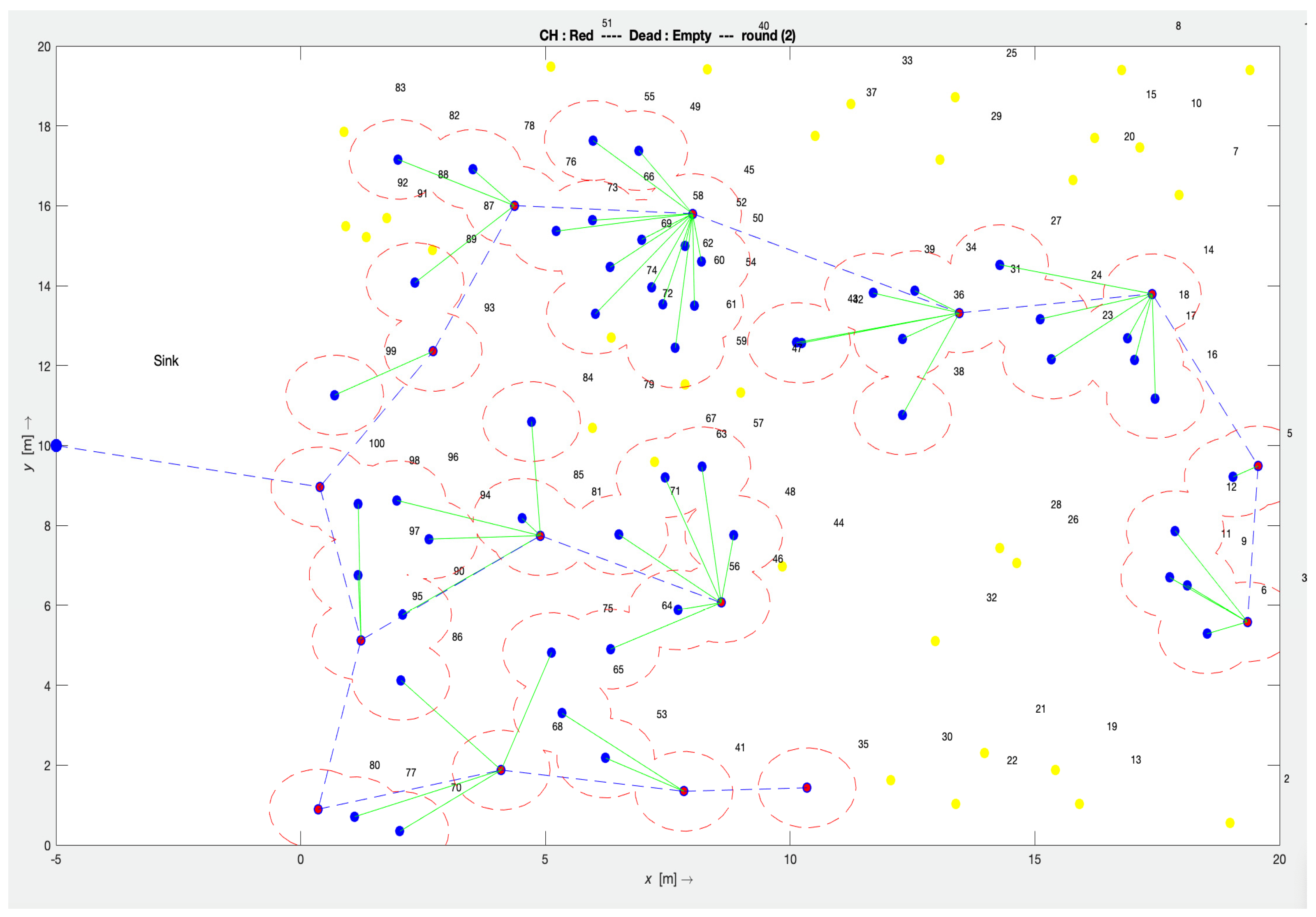
Figure 4 demonstrates the simulation experiment of the SOFM node-scheduling algorithm with 100 homogenous nodes i.e., having the same capabilities (sensing, communicating, power battery, processing power).
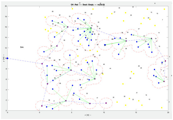
Figure 4.
SOFM simulation setup in MATLAB (Red—cluster head, Blue—child node, Yellow—dead node).
As mentioned earlier, the SOFM node-scheduling algorithm was compared to the BAT node-scheduling algorithm. It is worth noting that other node-scheduling algorithms were not included in this comparative analysis with the SOFM node-scheduling algorithm as they were demonstrated in our previous work, for example, how the BAT algorithm outperforms the randomized coverage node-scheduling algorithm (RCS) [23] and HMM node-scheduling algorithm [1]. Therefore, with the improvements shown by the SOFM over the BAT algorithm, it can be deduced that the newly proposed SOFM node-scheduling algorithm also outperforms the RCS and the HMM node-scheduling algorithms.
The simulation was individually tested 30 times, where one-way ANOVA analysis was implemented on both the SOFM and the BAT node-scheduling algorithms to identify the p-value for the statistical analysis. The statistical results are shown in Table 1.

Table 1.
Statistical analysis.
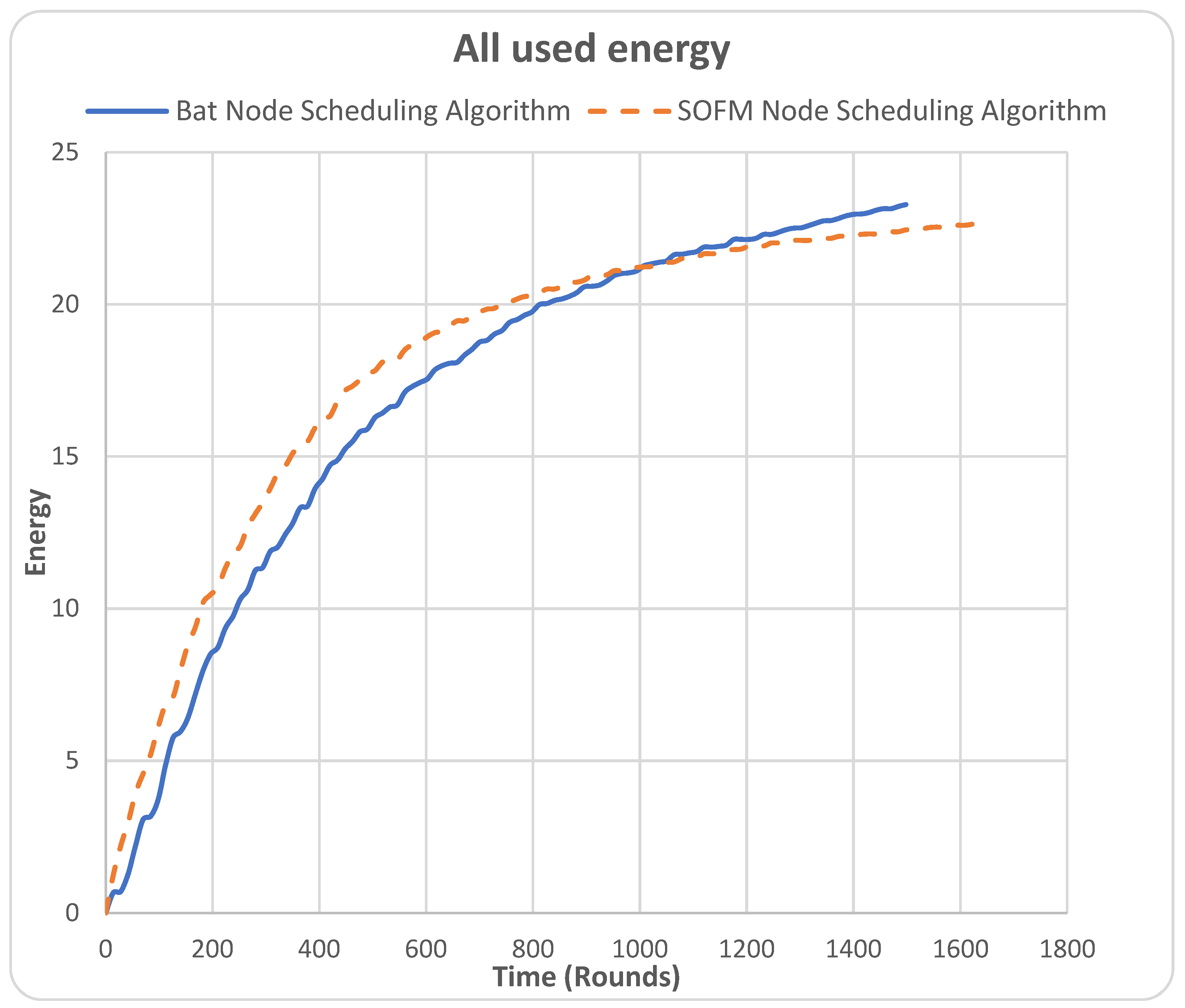
4.1. All Used Energy
The all used energy metric refers to the energy consumed by the nodes throughout the simulation time until all nodes fully deplete/consume their energy. In Figure 5, the X-axis represents time in round units, and the Y-axis is the energy used in Joule.
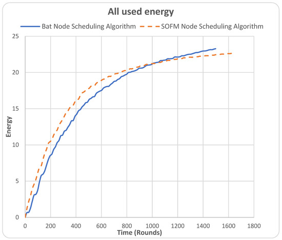
Figure 5.
All used energy.
For this metric, the SOFM node-scheduling algorithm resulted in less collective energy consumption by the WSN nodes and lasted for more rounds, i.e., up to 1638 rounds, while the BAT node-scheduling algorithm lasted up to 1498 rounds. This shows the SOFM node-scheduling algorithm extended the network’s lifetime more than the BAT algorithm. Despite these results, the BAT node-scheduling algorithm consumed less energy during the first half of the simulation. For instance, as can be noticed in the 42 rounds for the BAT node-scheduling algorithm, the amount of energy used is 1.28 joules, in contrast to the amount of energy used in the SOFM node-scheduling algorithm, which is 2.97 joules. However, it is worth mentioning that the SOFM node-scheduling algorithm at around 1000 depleted energy at a faster pace compared to the BAT node-scheduling algorithm due to the spatial configuration, which is based on the residual energy of each node. This can be improved through the utilization of a time series analysis model such as long short-term memory (LSTM).
4.2. Lifetime of Sensor Nodes
The lifetime of sensor nodes metric represents the number of live sensor nodes in the network during the simulation rounds. In this metric, the Y-axis represents the number of alive sensor nodes, while the X-axis represents times in rounds, as shown in Figure 6.
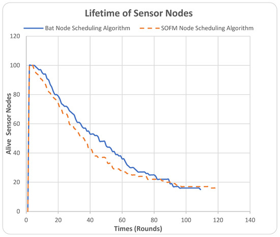
Figure 6.
Lifetime Sensor Nodes.
Initially, both algorithms in the WSN started their operation with 100 nodes. It can be noted from Figure 6 that the SOFM node-scheduling algorithm falls below the BAT node-scheduling algorithm from round 0 up to 85 rounds. This is not a disadvantage of the SOFM node-scheduling algorithm because the higher the number of live sensors, the higher the energy consumption, which is an undesired result. It can be noticed that the BAT node-scheduling algorithm fully depletes its energy at 108 rounds, where it is recorded to have only 15 nodes alive, and where the simulation threshold is set to finish, i.e., when the number of nodes reaches 15. In contrast, the SOFM node-scheduling algorithm has maintained the live sensors for a longer period, until round 118, which is an advantage by 10 rounds over the BAT node-scheduling algorithm. The advantage the SOFM node-scheduling algorithm has over the BAT node-scheduling algorithm in improving the nodes’ lifetime is due to the spatial feature it has in visualizing the best network configuration. The SOFM node-scheduling algorithm provides a solution that considers the residual energy of the nodes. However, a notable observation of the comparison between the two curves of the two algorithms is that the SOFM node-scheduling algorithm falls below the BAT node-scheduling algorithm and, hence, consumes more energy. This is due to the spatial distribution of energy. This confirms our initial observation in Section 4.1.
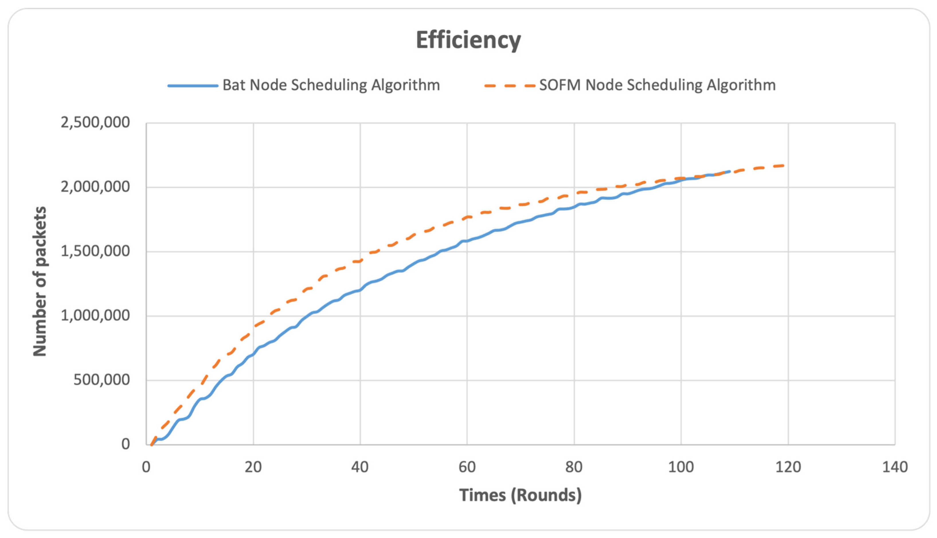
4.3. Efficiency
The efficiency metric is a measure of the network’s bandwidth that is used to determine the number of packets generated in the network. The lower the bandwidth, the lower the congestion and the fewer the data generated. In contrast, the higher the bandwidth, the higher the congestion and the more the data generated. The X-axis represents the number of rounds, while the Y-axis represents the number of packets in the network. The primary focus lies on the volume of packets transmitted and received within the WSN, as shown in Figure 7.
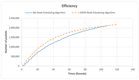
Figure 7.
Efficiency.
After 110 rounds, it can be noticed that the SOFM node-scheduling algorithm has recorded a higher efficiency with extended efficiency-lifetime too whereas the BAT node-scheduling algorithm recorded a network lifetime at the 110 round (died) as can be noted in Figure 7. The SOFM node-scheduling algorithm has the larger number of packets sent/received in the network which indicates better connectivity and lifetime of the network.
4.4. Connectivity
The connectivity metric quantifies to which extent nodes are connected in the network. In Figure 8, the Y-axis is the performance of connectivity which is measured by number as a value fraction of nodes connected in the network and the X-axis is the number of rounds. For example, in the simulation, there are 100 nodes in the network when the connectivity factor reaches 0.98. This indicates that the total number of the connected nodes is 98 out of 100.
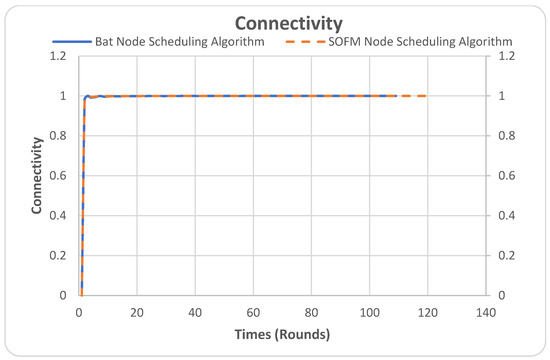
Figure 8.
Connectivity.
It can be noticed that both algorithms performed similarly well during the simulation period, except for the SOFM node-scheduling algorithm’s extended network lifetime. As can be noticed, the BAT node-scheduling algorithm stopped/died at 108 rounds, whereas the SOFM node-scheduling algorithm continues its lifecycle until round 118.
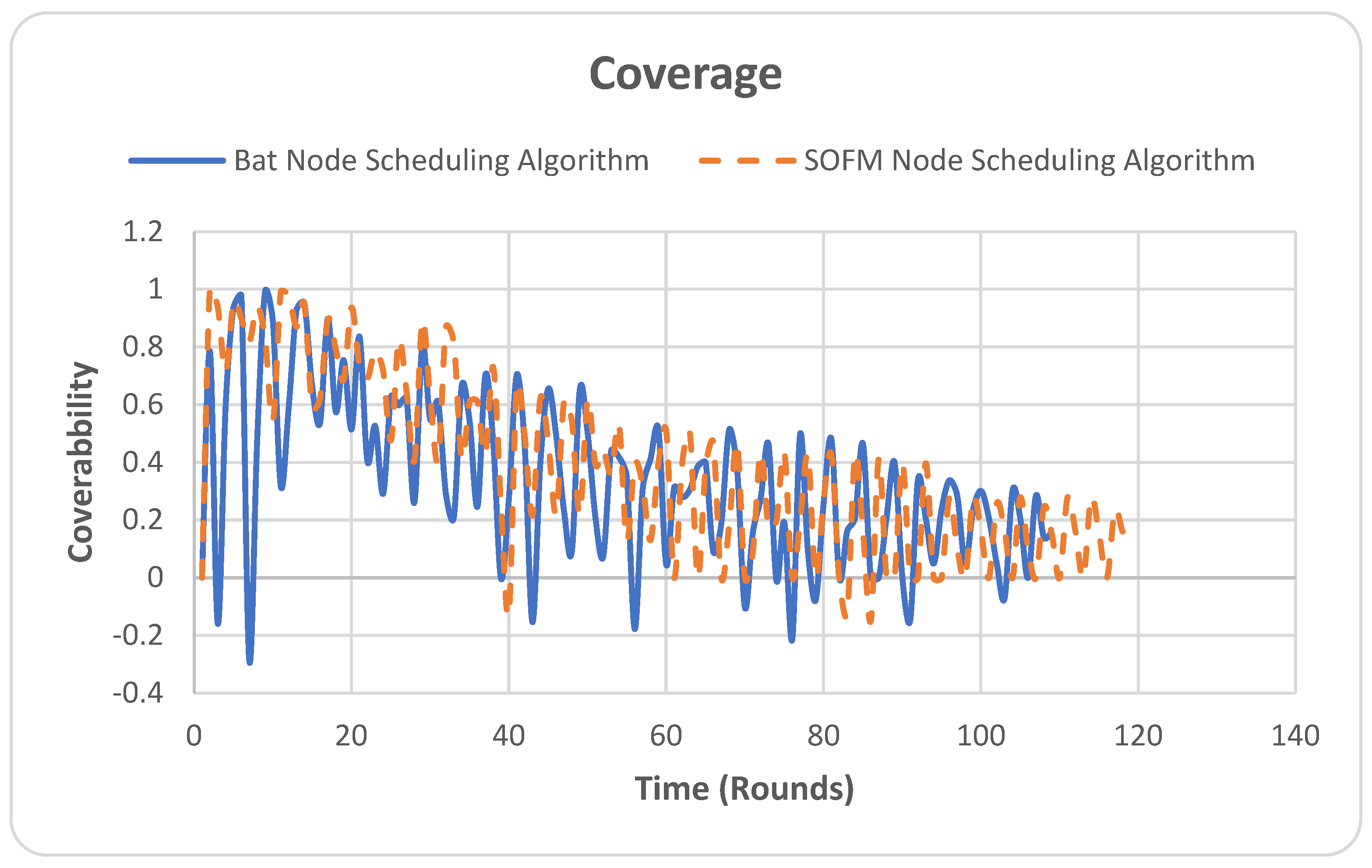
4.5. Coverage
The coverage metric represents the extent to which an area to be monitored is covered. In Figure 9, the Y-axis is the performance of coverage, which is measured by the number as a value fraction of nodes connected in the network, and the X-axis is the number of simulation rounds. In the simulation, the coverage is represented by the fraction of the area covered by the network. For example, if the area of the test field is 100 m2, a coverage of 0.8 value would mean 80 m2 has been covered.

Figure 9.
Coverage.
As can be noted in Figure 9, the overall coverage fluctuates as time progresses, and as nodes run out of energy, the coverage decreases. Similarly, the coverage of the BAT node-scheduling algorithm falls after 108 rounds, where all nodes run out of energy; thus, no coverage is seen. The SOFM node-scheduling algorithm outperformed the BAT node-scheduling algorithm coverage by 10 rounds. This is due to the spatial configuration considered by the SOFM node-scheduling algorithm in its core design. However, this fluctuation can be controlled through the utilization of a time series model (e.g., LSTM), where a sequence of good coverage values based on time can be found and then replicated throughout the lifetime of the WSN.
5. Conclusions
This paper addressed the MOO problem in which a trade-off between requirements is obtained to provide reliable performance in safety-critical systems in the WSN. The contribution is a novel node-scheduling algorithm based on the SOFM model to provide the optimal solution for WSNs. Accordingly, the achieved results always provided an extended coverage and network lifetime while maintaining the same level of connectivity in comparison to the BAT node-scheduling algorithm. This, in turn, improved service availability and reliability for improved dependable WSN safety-critical systems. The self-organizing capacity in the SOFM node-scheduling algorithm outperformed the BAT node-scheduling algorithm through its simplistic method of dimension reduction and classification. While the spatial feature of the SOFM node-scheduling algorithm enabled a better representation of the WSN configuration, the data representations may be abstracted due to the migration from spatial to temporal spaces. In future work, this limitation will be addressed by introducing the LSTM model, whose approach is based entirely on a time-dependent framework. Although the metrics involved in this research are concerned with the MOO problem, in future work we will look thoroughly at metrics that are concerned with real-time system applications to robustly assess the proposed SOFM node-scheduling algorithm. For example, our hypothesis will extend to propose an approach that approximates the end-to-end delay distribution of the links between immediate nodes. This shall enable certain sequences of messages to be sent through a chain of selected paths within time intervals and thereby enable the application of WSNs to exploit the QoS trade-off based on timeliness requirements.
Author Contributions
Methodology, I.A.-N. and A.L.; Software, I.A.-N.; Validation, I.A.-N.; Formal analysis, I.A.-N. and A.L.; Investigation, I.A.-N. and R.R.; Resources, I.A.-N.; Data curation, I.A.-N.; Writing—original draft, I.A.-N.; Writing—review & editing, I.A.-N., A.L. and R.R. All authors have read and agreed to the published version of the manuscript.
Funding
This research received no external funding.
Data Availability Statement
Data are contained within the article.
Acknowledgments
The authors express their gratitude to everyone who took part in the accomplishment of this project. A heartfelt appreciation goes out to the Faculty of Science and Technology at Middlesex University for their unwavering support throughout all phases of the research.
Conflicts of Interest
The authors declare no conflict of interest.
References
- Alnader, I.; Lasebae, A.; Raheem, R. Using Hidden Markov Chain for Improving the Dependability of Safety-Critical WSNs’. In International Conference on Advanced Information Networking and Applications; Springer: Berlin/Heidelberg, Germany, 2023; pp. 460–472. [Google Scholar]
- Sohraby, K.; Minoli, D.; Znati, T. Wireless Sensor Networks: Technology, Protocols, and Applications; John Wiley & Sons: Hoboken, NJ, USA, 2007. [Google Scholar] [CrossRef]
- Rausand, M. Reliability of Safety-Critical Systems: Theory and Applications; John Wiley & Sons: Hoboken, NJ, USA, 2014. [Google Scholar] [CrossRef]
- Knight, J.C. Safety critical systems: Challenges and directions. In Proceedings of the 24th International Conference on Software Engineering, Orlando, FL, USA, 19–25 May 2002; pp. 547–550. [Google Scholar] [CrossRef]
- Aslan, Y.E.; Korpeoglu, I.; Ulusoy, Ö. A framework for use of wireless sensor networks in forest fire detection and monitoring. Environ. Urban Syst. 2012, 36, 614–625. [Google Scholar] [CrossRef]
- Coronato, A.; Testa, A. Approaches of Wireless Sensor Network Dependability Assessment. In Proceedings of the 2013 Federated Conference on Computer Science and Information Systems, Krakow, Poland, 8–11 September 2013; pp. 881–888. Available online: http://ieeexplore.ieee.org/xpls/abs_all.jsp?arnumber=6644115 (accessed on 28 June 2015).
- Avižienis, A.; Laprie, J.-C.; Randell, B.; Landwehr, C. Basic concepts and taxonomy of dependable and secure computing. IEEE Trans. Dependable Secur. Comput. 2004, 1, 11–33. [Google Scholar] [CrossRef]
- Meier, A. Safety-Critical Wireless Sensor Networks; Swiss Federal Institute of Technology Zurich: Zürich, Switzerland, 2009. [Google Scholar] [CrossRef]
- Purushothaman, K.E.; Nagarajan, V. Multiobjective optimization based on self-organizing Particle Swarm Optimization algorithm for massive MIMO 5G wireless network. Int. J. Commun. Syst. 2021, 34, e4725. [Google Scholar] [CrossRef]
- Al-Nader, I.; Lasebae, A.; Raheem, R.; Khoshkholghi, A. A Novel Scheduling Algorithm for Improved Performance of Multi-Objective Safety-Critical Wireless Sensor Networks Using Long Short-Term Memory. Electronics 2023, 12, 4766. [Google Scholar] [CrossRef]
- Taleb, A.A. Sink mobility model for wireless sensor networks using Kohonen self-organizing map. Int. J. Commun. Netw. Inf. Secur. 2021, 13, 62–67. [Google Scholar] [CrossRef]
- Sharma, N.K.; Tiwari, P.K.; Sood, Y.R. Review of artificial intelligence techniques application to dissolved gas analysis on power transformer. Int. J. Comput. Electr. Eng. 2011, 3, 577–582. [Google Scholar] [CrossRef]
- Mittal, M.; Kumar, K. Energy Efficient Homogeneous Wireless Sensor Network Using Self-Organizing Map (SOM) Neural Networks. Afr. J. Comput. ICT 2015, 8, 179–184. [Google Scholar]
- Kohonen, T. Essentials of the self-organizing map. Neural Netw. 2013, 37, 52–65. Available online: https://www.sciencedirect.com/science/article/pii/S0893608012002596 (accessed on 27 October 2023). [CrossRef] [PubMed]
- Zhang, Z.; Zhang, C.; Li, M.; Xie, T. Target positioning based on particle centroid drift in large-scale WSNs. IEEE Access 2020, 8, 127709–127719. [Google Scholar] [CrossRef]
- Miljković, D. Brief review of self-organizing maps. In Proceedings of the 2017 40th International Convention on Information and Communication Technology, Electronics and Microelectronics (MIPRO), Opatija, Croatia, 22–26 May 2017; pp. 1061–1066. [Google Scholar] [CrossRef]
- Cordina, M.; Debono, C.J. Increasing wireless sensor network lifetime through the application of SOM neural networks. In Proceedings of the 2008 3rd International Symposium on Communications, Control and Signal Processing, St. Julians, Malta, 12–14 March 2008; pp. 467–471. [Google Scholar] [CrossRef]
- Chen, Z.; Li, S.; Yue, W. SOFM neural network based hierarchical topology control for wireless sensor networks. J. Sens. 2014, 2014, 121278. [Google Scholar] [CrossRef]
- Xie, T.; Zhang, C.; Zhang, Z.; Yang, K. Utilizing active sensor nodes in smart environments for optimal communication coverage. IEEE Access 2018, 7, 11338–11348. [Google Scholar] [CrossRef]
- Bai, R.G.; Qu, Y.G.; Zhao, B.H.; Lin, Z.T.; Yang, C.M. Intelligent Monitoring Scheduling in Wireless Sensor Networks. In Proceedings of the 2008 4th International Conference on Wireless Communications, Networking and Mobile Computing, Dalian, China, 12–17 October 2008; pp. 1–4. [Google Scholar] [CrossRef]
- Patra, C.; Roy, A.G.; Chattopadhyay, S.; Bhaumik, P. Designing Energy-Efficient Topologies for Wireless Sensor Network: Neural Approach. Int. J. Distrib. Sens. Netw. 2010, 6, 216716. [Google Scholar] [CrossRef]
- Talei, H.; Benhaddou, D.; Gamarra, C.; Benhaddou, M.; Essaaidi, M. Identifying Energy Inefficiencies Using Self-Organizing Maps: Case of A Highly Efficient Certified Office Building. Appl. Sci. 2023, 13, 1666. [Google Scholar] [CrossRef]
- Liu, C.; Wu, K.; Xiao, Y.; Sun, B. Random coverage with guaranteed connectivity: Joint scheduling for wireless sensor networks. IEEE Trans. Parallel Distrib. Syst. 2006, 17, 562–575. [Google Scholar] [CrossRef]


Disclaimer/Publisher’s Note: The statements, opinions and data contained in all publications are solely those of the individual author(s) and contributor(s) and not of MDPI and/or the editor(s). MDPI and/or the editor(s) disclaim responsibility for any injury to people or property resulting from any ideas, methods, instructions or products referred to in the content. |
© 2023 by the authors. Licensee MDPI, Basel, Switzerland. This article is an open access article distributed under the terms and conditions of the Creative Commons Attribution (CC BY) license (https://creativecommons.org/licenses/by/4.0/).