Multi-Modal Contrastive Learning for LiDAR Point Cloud Rail-Obstacle Detection in Complex Weather

Abstract

Obstacle intrusion is a serious threat to the safety of railway traffic. LiDAR point cloud 3D semantic segmentation (3DSS) provides a new method for unmanned rail-obstacle detection. However, the inevitable degradation of model performance occurs in complex weather and hinders its practical application. In this paper, a multi-modal contrastive learning (CL) strategy, named DHT-CL, is proposed to improve point cloud 3DSS in complex weather for rail-obstacle detection. DHT-CL is a camera and LiDAR sensor fusion strategy specifically designed for complex weather and obstacle detection tasks, without the need for image input during the inference stage. We first demonstrate how the sensor fusion method is more robust under rainy and snowy conditions, and then we design a Dual-Helix Transformer (DHT) to extract deeper cross-modal information through a neighborhood attention mechanism. Then, an obstacle anomaly-aware cross-modal discrimination loss is constructed for collaborative optimization that adapts to the anomaly identification task. Experimental results on a complex weather railway dataset show that with an mIoU of 87.38%, the proposed DHT-CL strategy achieves better performance compared to other high-performance models from the autonomous driving dataset, SemanticKITTI. The qualitative results show that DHT-CL achieves higher accuracy in clear weather and reduces false alarms in rainy and snowy weather.

1. Introduction

Railways play an important economic and social role in transport. Obstacle intrusions, e.g., caused by geological hazards within the rail track area, animals, vehicles, objects falling from bridges above the tracks, etc., can seriously jeopardize the safety of rail traffic. With the development of light detection and ranging (LiDAR) technology and deep learning-based environmental perception methods, rail transport has become more intelligent in recent years. Point cloud 3D semantic segmentation (3DSS) provides a new method for unmanned rail-obstacle detection. Based on 3DSS, Wang [1], Soilán [2], Manier [3], and Dibari [4] achieved rail-obstacle detection through a point-by-point analysis of railway point clouds and established an intelligent railway monitoring system. However, railways are mostly located in the wilderness and are exposed to complex weather conditions, which inevitably degrades the performance of models and hinders their real-world application.

To cope with the effects of complex weather, filter-based methods [5,6,7] pre-process the input data and remove the noise caused by rain or snow shading to maintain performance. Following the same principle, simulation-based methods [8,9] synthesize scattered noise representing rain, snow, or fog into clear weather data as a form of data augmentation to improve the adaptability of recognition neural networks. In addition, in our practical application, we found that the main factor leading to classification confusion in rain and snow is changes in the reflectivity of the surface of the object. As shown in Figure 1, because of the increase in specular reflection when the rail metal surface is wet, the contrast of the positive incidence region increases, and no return light is detected in the grazing region, resulting in partially missing imaging. Also, snow leads to increased diffuse reflections. Overall, dramatic changes in the light-intensity distribution of point clouds will occur in rain and snow, as shown in Figure 2. Both figures come from our real-world data collection. In a word, the data distribution is drastically and irregularly shifted with respect to clear weather data, resulting in the degradation of model performance, mainly in the form of an increase in false alarms, which cannot be resolved by using a filter-based approach.

Sensor fusion methods [10,11,12,13,14,15,16,17,18,19,20] have been employed to improve adaptability to complex environments, using the camera to obtain high-resolution object texture information to compensate for the shortcomings of sparse and coarse LiDAR point clouds. However, RGB images undergo dramatic fluctuations in brightness and contrast in complex weather due to the light-sensitive nature of the camera, with the same characteristics as point cloud reflectivity, resulting in more difficult model fitting. In contrast, we demonstrate that local geometric structure information is a more reliable reference for a deep learning-based method. The neighborhood relationship captured from the different perspectives of the camera and LiDAR sensors is key to the higher robustness of multi-modal methods in complex weather. As shown in Figure 3, there is a difference in the receptive fields of 3D and 2D networks, i.e., the anchor point has a different influence on the neighborhood points during the back-propagation training stage.

In this paper, we propose a neighborhood attention-driven multi-modal contrast learning strategy, named DHT-CL, to improve the performance of rail-obstacle detection based on 3DSS in complex weather. Our approach has the following advantages: (1) It makes full use of the neighborhood information from the different perspectives of the camera and LiDAR sensors, which is robust to object reflectance variations in complex weather. (2) Only point cloud input is required during the inference stage, without the need for image input, making it efficient for deployment. (3) It improves the general rain and snow resistance of deep learning-based methods, which cannot be addressed by using filter-based data pre-processing methods alone.

The framework can be explained as follows: First, using the point cloud and image as input, 2D and 3D feature maps are independently extracted by the 2D and 3D backbones, respectively. Second, a Dual-Helix Transformer (DHT) module reassigns weights to 2D and 3D features based on a neighborhood attention mechanism, which allows for selective preservation or filtering of homogeneity or heterogeneity in neighborhood cross-modal information. Third, an adaptive cross-modal discrimination loss is constructed for collaborative optimization, which softens or sharpens the output logit distribution depending on the presence or absence of obstacle anomalies. This structure is adaptive to learning priorities. It also allows 2D branches to be discarded during the inference stage and achieves performance improvements that are not limited to overlapping field-of-view (FOV) regions. Finally, based on a complex weather railway dataset with point-wise annotation, we compare our method with state-of-the-art models [19,21,22,23,24] from the autonomous driving dataset, SemanticKITTI [25]. The experimental results show that our DHT-CL method achieves a higher mIoU of 87.38% compared to the other models. The qualitative results show that DHT-CL improves accuracy in clear weather and reduces false alarms in rain and snow.

The contributions of this paper can be summarized as follows:

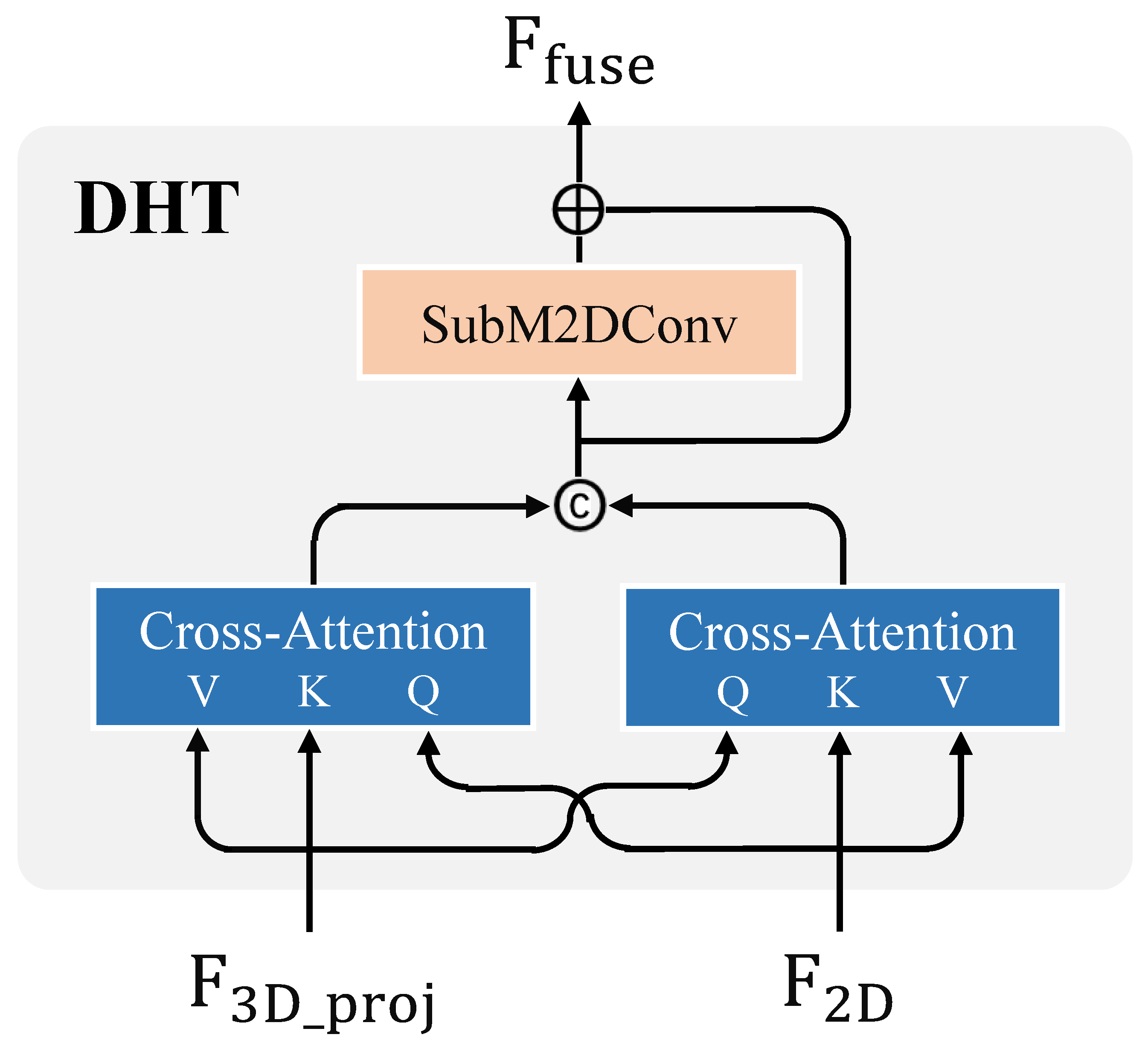
• A Dual-Helix Transformer (DHT) module is proposed to extract deeper information for robust sensor fusion in complex weather through local cross-attention mechanisms.
• An adaptive contrastive learning strategy is achieved through the use of an obstacle anomaly-aware cross-modal discrimination loss, which adjusts the learning priorities according to the presence or absence of obstacles.
• Based on the proposed semantic segmentation network, a rail-obstacle detection method is implemented to identify and locate multi-class unknown obstacles (minimum size $7\times 7\times 7$ cm${}^3$) in complex weather, which exhibits high accuracy and robustness.

The remainder of this paper is organized as follows. We review the related works in Section 2 and describe our proposed method in Section 3. Section 4 presents the experimental setup and results, and we conclude this paper in Section 5.

2. Related Works

This section briefly reviews the related works, which are divided into four categories: rail-obstacle detection, 3D environmental perception in adverse weather, sensor fusion, and multi-modal contrastive learning.

2.1. Rail-Obstacle Detection

Previous railway-obstacle detection studies have relied on different types of sensors, i.e., leaky cables [26], vibrating fibers [27], ultrasonic [28], millimeter-wave radar [29], infrared cameras [30], RGB cameras [31,32,33,34,35,36,37,38,39,40], and LiDAR. Contact detection methods [26,27] face the problem of excessive volume. Ultrasonic [28] and millimeter-wave radar [29] operate over long distances but with low resolution.

Extensive studies have used RGB cameras due to their high resolution and low cost. In addition, some studies [30] have combined RGB and infrared cameras to work in low-light conditions. For 2D input data, conventional image processing methods detect the rail track lines and nearby obstacles using the Hough transform [31,32,33] or the Canny or Sobel operators [34]. The optical flow-based method [41] and Kalman filtering-based method [29] have been used for motion obstacle detection. Moreover, deep learning-based methods have shown advantages in terms of accuracy and robustness, and many studies have followed the framework of single-stage YoLo [35,36,37] or two-stage RCNN [38,39] for object detection. Other studies have relied on semantic segmentation, focusing on rail track lines [40] or railway track area segmentation [42]. In [40], the authors incorporated vanishing point detection and identified shaded rail track points as obstacles. In [30], the authors detected anomalies using GAN [43] reconstruction and comparison to issue obstacle alarms.

Overall, both IR and RGB camera-based methods face difficulties in measuring distance and are prone to false alarms for objects in safe positions due to the perspective relationship. RGB cameras deteriorate dramatically in low-light conditions, whereas infrared cameras can work at night but have inferior image quality. Additionally, methods based on object detection algorithms mostly simulate obstacles using specific known classes such as pedestrians, vehicles, and specific target shapes. Actually, object detection algorithms are only effective for detecting objects with specific and consistent features and cannot be used for detecting multi-class novel obstacles. These methods lack generalized evaluation criteria, whereas our segmentation-based framework enables multi-class obstacle detection in more complex scenarios.

LiDAR has proven its effectiveness in 3D perception in recent years. LiDAR-based obstacle detection methods start with railway track localization and can be divided into geometric-based methods, machine learning-based methods, and deep learning-based methods. Geometric-based methods filter track points by searching for height and intensity jumps [44,45], implementing Hough transformations on BEV projections [46], or judging based on gauge corner characteristics [47]. The track curve is then fitted using RANSAC [45], multi-segment folding lines [44], or an eigenvector-based neighborhood growth algorithm [46]. In machine learning methods [48,49], rail track lines are extracted through classification. The feature mapping is performed using principal component analysis (PCA), whereas classification is performed using linear discriminant analysis (LDA) [48] or support vector machines (SVMs) [49]. Yu et al. [50] adopted cylinder voxel partitioning and implemented 3D convolutions. Wang et al. [51] conducted 2D convolutions on the spherical projection of railway point clouds and incorporated an attention mechanism with decoupled spatial and channel-wise aspects. Based on rail track localization, Qu et al. [52] removed background points in the region of interest (RoI) and obtained outlier point clusters through Euclidean clustering for obstacle alarms. Another branch of research is devoted to full-scene railway perception based on semantic segmentation. Manier [3] designed a point-based axisymmetric convolution operator that projects the point cloud into 2D along the axis of symmetry in a columnar neighborhood. This method performs 2DCNN, which can accommodate railway scenes with significant vertical differences and minor horizontal differences. Dibari et al. [4] first applied the point cloud semantic segmentation networks PointNet [53] and PointNet++ [54] for railway scene parsing. The former achieved a higher mIoU of 62.6%. Soilán et al. [2] ported PointNet [53] and KPConv [55] to railway scenes, but they achieved satisfactory results only on regular concrete pavements in railway tunnels.

Methods based on clustering and outlier removal work well in experiments but are unstable in the real world. This requires careful thresholding for diverse scenarios, otherwise a large number of false alarms can occur due to fitting errors. Existing semantic segmentation models in railway scenes generally have unsatisfactory performance and suffer from performance degradation in rainy and snowy conditions. Our method improves accuracy and robustness in both clear and adverse weather conditions through multi-modal contrastive learning.

2.2. Two-Dimensional Environmental Perception in Adverse Weather

Hussain et al. [56] identified the occurrence of extreme weather-induced anomalies in autonomous driving systems based on GAN-reconstructed pixel errors. Their experiments showed that the performance of camera-based perception systems drastically decreases in complex weather conditions (rain, fog, snow, etc.). Liu et al. [57] proposed a camera and millimeter-wave radar fusion approach to enhance the performance of vehicle detection and trajectory predictions in complex weather. Their experimental results showed that the single-sensor approach is prone to producing missed alarms in extreme weather. Similarly, the authors of [58] also explored the manifestations of the failures of single-camera sensor-based methods and proposed a method based on prediction variance and trajectory deviations to eliminate false alarms.

Previous studies have shown that end-to-end neural network models that rely solely on camera sensors suffer from dramatic performance degradation in adverse weather conditions.

2.3. Three-Dimensional Environmental Perception in Adverse Weather

Point cloud distortion due to rain and snow is a direct cause of the performance degradation of LiDAR-based environmental perception methods. Full reference metrics for evaluating point cloud distortion rely on assessing the similarity between the distorted point cloud and the original point cloud based on the topology, geometry, color features [59,60], local curvature statistics [61], or 3D edge features [62]. Since the original point cloud is not always accessible, no reference metrics are proposed based on the 3D natural scene statistics and entropy [63] or neural networks [64]. Furthermore, Viola et al. [65] extracted a subset of statistical features from the original point cloud for reduced-reference evaluation, and Zhou et al. [66] proposed a reduced-reference metric based on content-oriented similarity and statistical correlation measurements.

To address point cloud distortion, Le et al. proposed an adaptive noise-removal filter [5] for the range image projected from LiDAR point clouds and an adaptive group of density outlier-removal filters [6] for LiDAR point clouds. In addition, Wang et al. [7] proposed a dynamic distance-intensity outlier-removal filter for snow denoising to pre-process point clouds and remove noise caused by adverse weather. Mai et al. [8] synthesized fog on the KITTI dataset to generate images and point clouds with reduced visibility, while Shih et al. [9] proposed a multi-mechanism spray synthesis model to improve the performance of recognition models. Kim et al. [67] analyzed the reasons for imaging performance degradation in adverse weather conditions by testing LIDAR’s imaging capability of a 0.6 × 0.6 m${}^2$ square target under varying degrees of rain and fog. The performance of multiple sets of LiDAR sensors under different artificial rainfall conditions was also evaluated in [68], using the number of imaging points of the target as a criterion. Piroli et al. [69] detected the presence of rain and snow using an energy-based anomaly detection framework. Li et al. [70] evaluated and modeled LiDAR visibility under different artificial fog conditions, while Delecki et al. [71] increased pressure on the recognition model by gradually adding computer-synthesized rain, snow, and fog to analyze the causes of recognition failures.

Based on the aforementioned analyses, we designed a multi-modal contrastive learning strategy specifically for rain and snow to alleviate performance degradation due to changes in object reflectivity in adverse weather, which cannot be resolved using filter-based approaches.

2.4. Sensor Fusion Methods

Sensor fusion methods attempt to fuse camera and LiDAR information and exploit their complementarity. Typically, 3D point clouds are first converted to 2D through perspective projection, spherical projection, cylindrical projection, or bird’s-eye-view (BEV) projection. Snapnet [10] takes both types of 2D and 3D data as input to the network, which is data-level fusion. FuseSeg [11,12] concatenate the embedding layer features from the 2D and 3D modals, which is feature-level fusion. Genova et al. [13] designed a sparse filter and reprojected 2D images to 3D point clouds to facilitate the training of 3D models with 2D labels. Pointpainting [14] paints the point clouds according to the images, adding RGB channels to the 3D data. SAT [15] is a 2D-assisted training strategy that uses 2D images to build an attention map during the training stage while skipping the 2D branch using an attention mask during the inference stage. In MSeg3D [18] the non-overlapping region is complemented with predicted pseudo-camera features and self- and cross-attention between the camera, LiDAR, and fusion features are performed to generate the final prediction scores.

However, these methods necessitate precise alignment of the point cloud and image and performance enhancements only occur in the overlapping FOV region.

2.5. Multi-Modal Contrastive Learning

Contrastive learning across modalities promotes multi-modal information transformation and allows image branches to be discarded during the inference phase. In PMF [16], the embedding layer features are aggregated, and a modality perception loss is constructed using the KL divergence function to co-optimize. Liu et al. [17] generated fusion features using a linear module, which contains element-wise multiplication and addition, and then aligned the fusion features and 2D features using the L2 loss function for training. In 2DPASS [19], knowledge distillation [72] is implemented on a multi-scale feature map in a multilayer perceptron (MLP) manner. In SSLp2i [20], the embedding features in the FOVs are used to construct a contrastive loss using the L2 norm for semi-supervised learning.

Following the method that builds a contrastive loss for collaborative optimization, we developed a more effective method for information transfer in complex weather conditions while simultaneously optimizing obstacle anomaly detection tasks.

3. Methods

The objective of this study is to improve point cloud 3DSS performance in complex weather for rail-obstacle detection. We propose a multi-modal contrastive learning strategy, named DHT-CL, to handle the difficulty of data distribution shifts due to object surface reflectivity changes in complex weather.

An overview of the framework of DHT-CL is shown in Figure 4. Specifically, during the training stage, both point cloud and image branches are activated, and 2D and 3D features are first extracted independently by the 2D and 3D encoding networks, respectively. Then, the 3D features are projected into 2D to generate pseudo-2D features. The pseudo-2D and 2D features are then fed into the DHT module simultaneously to obtain the fusion features. Then, the 3D and fusion features are decoded by two independent classifiers to output the prediction scores, between which an obstacle anomaly-aware modality discrimination loss is constructed for collaborative optimization. All of the above are supervised by pure 3D labels. During the inference stage, the 2D branch is masked, which reduces the computational burden.

The 2D backbone is a U-net for semantic segmentation. It contains a downsampling layer of a pre-trained ResNet34 [73], an upsampling layer based on transpose convolutions, and a skip-connected structure with a hidden size of 64. The 3D extractor, known as SPVCNN [23], is also a U-net with a voxel size of 0.05 m and a hidden size of 64.

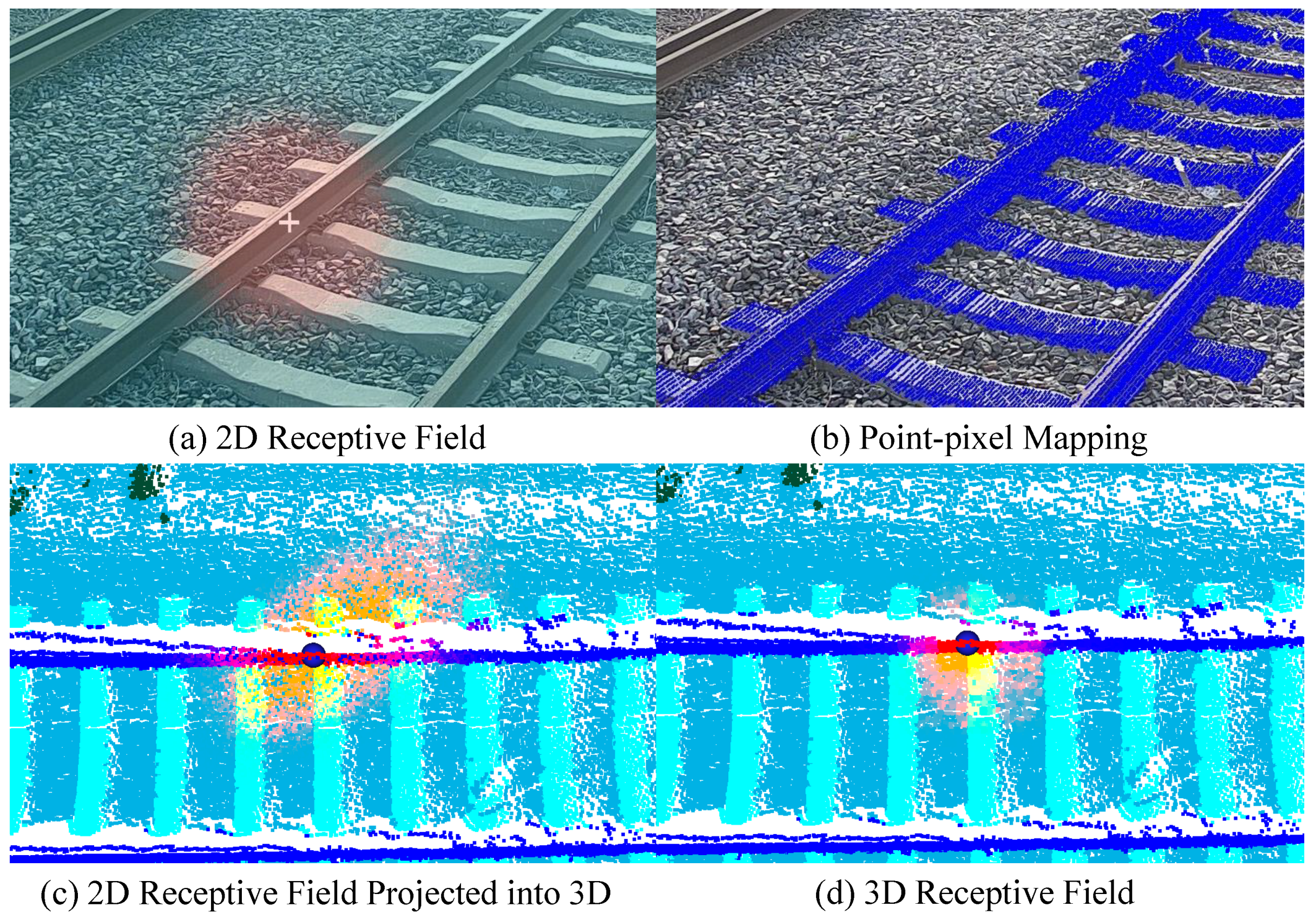
3.1. Point-Pixel Mapping

The point-pixel correspondence serves as crucial prior knowledge in multi-modal methods and has a significant influence on the subsequent predictions. Instead of directly mapping the input 3D point clouds into 2D space, we first establish a pairwise index of the point cloud and the image within the overlapping FOV region. Then, we map the 3D features to 2D space based on this index, thereby generating pseudo-2D features.

Perspective projection is adopted in this paper to create the 2D-3D mappings. Specifically, given a LiDAR point cloud $P={\left\{p_i\right\}}_{i=1}^N\in {\mathbb{R}}^{N\times 4}$, a single point is denoted as $p_i={\left\{x_i,y_i,z_i,I_i\right\}}_{i=1}^N\in {\mathbb{R}}^4$, an RGB image is denoted as $Q={\left\{q_{u,v}\right\}}_{u,v=1}^{U,V}\in {\mathbb{R}}^{U\times V\times 3}$, and a single pixel is denoted as $q_{u,v}=\left\{r_{u,v},g_{u,v},b_{u,v}\right\}\in {\mathbb{R}}^3$. The projection relationship is expressed as:

$${\left[u,v,1\right]}^T=\frac{1}{z_i}\times K\times T\times {\left[x_i,y_i,z_i,1\right]}^T$$

(1)

where K and T are the pre-calibrated camera internal matrices $K\in {\mathbb{R}}^{3\times 4}$ and the external matrices $T\in {\mathbb{R}}^{4\times 4}$. In this work, K is obtained using the calibration method proposed by Zhang [74], and T is obtained using the method proposed by Yuan [75].

The 2D point clouds derived from the 3D projection are denoted as $P_{2D}={\left\{m_i,n_i\right\}}_{i=1}^N\in {\mathbb{R}}^{K\times 4}$. They are subsequently discretized based on the camera’s resolution r. The points within the camera picture $(H,W)$ are filtered as follows:

$${\left\{u_i^{{}^{\prime }},v_i^{{}^{\prime }}\right\}}_{i=1}^N={\left\{\left[\frac{m_i}{r}\right]\le H,\left[\frac{n_i}{r}\right]\le W\right\}}_{i=1}^N$$

(2)

Finally, the point-pixel correspondence index $Index\left\{\left(u,v\right),i\right\}$ is established based on whether the pixel coordinates ${\left\{u,v\right\}}_{u,v=1}^{U,V}$ overlap with the projected point cloud coordinates ${\left\{u_i^{{}^{\prime }},v_i^{{}^{\prime }}\right\}}_{i=1}^N$.

3.2. Dual-Helix Transformer

The DHT module is key to the proposed contrastive learning strategy. Previous methods for transferring information between different modalities or representations, such as knowledge distillation [72], 2DPASS [19], PVKD [21], and xMUDA [76], incorporate a learnable layer as a buffer, achieving better performance compared to naive direct fusion methods because the learnable module is able to compensate for modal heterogeneity differences. However, with the pull of the loss function, the learnable module has a tendency to make the transformed data distribution too similar to another modality, thereby compromising the heterogeneous information transfer. Differences between modalities can hinder information transfer, but they are also the real cause of performance improvements. Balancing the trade-off between homogeneity and heterogeneity is crucial for multi-modal methods. We observe that neighborhood relationships play a crucial role in cross-modal information transfer. For instance, the edges of an object are the same, regardless of whether it is described through an RGB image or XYZ coordinates, and are less affected by changes in intensity or color in rainy or snowy weather. The DHT module pre-processes the features to be fused based on a neighborhood attention mechanism. It searches for the neighboring points of a pixel in the pseudo-2D point cloud space, calculates a Gram matrix describing similarity, and adjusts the central element based on these weights. The same operation is performed for the pseudo-2D point cloud features. In this way, objects with weaker neighborhood relationships are assigned smaller weights, thereby eliminating some of the confusing information generated by perspective relationships, such as railway tracks that look like they are connected to a distant railway signal pole in a 2D image. At the same time, information with specific characteristics is extracted and encoded into the data. Although the feature maps in the two imaging perspectives are completely different, the local geometric structures are similar, resulting in higher relevant weights.

Figure 5 shows a schematic diagram of the DHT module. Specifically, the input of the DHT module is the 2D features, $F_{2D}$, extracted by the 2D network and the pseudo-2D features, $F_{3Dproj}$, projected by the 3D features. The output of the DHT module is the fusion features, $F_{fuse}$. The formulas are as follows:

$$F_{3Dproj}^{{}^{\prime }}=Softmax\left\{\frac{{\mathcal{L}}_Q\left(F_{3Dproj}\right){\mathcal{L}}_K{\left(F_{2D}\right)}^T}{\sqrt{d_k}}\right\}{\mathcal{L}}_V\left(F_{2D}\right)$$

(3)

$$F_{3Dproj}^{{}^{″}}=Layernorm\left\{F_{3Dproj}^{{}^{\prime }}+\mathcal{L}\left(F_{3Dproj}^{{}^{\prime }}\right)\right\}$$

(4)

$$F_{2D}^{{}^{\prime }}=Softmax\left\{\frac{{\mathcal{L}}_Q\left(F_{2D}\right){\mathcal{L}}_K{\left(F_{3Dproj}\right)}^T}{\sqrt{d_k}}\right\}{\mathcal{L}}_V\left(F_{3Dproj}\right)$$

(5)

$$F_{2D}^{{}^{″}}=Layernorm\left\{F_{2D}^{{}^{\prime }}+\mathcal{L}\left(F_{2D}^{{}^{\prime }}\right)\right\}$$

(6)

$$F_{fuse}=cat\left(F_{2D}^{{}^{″}},F_{3Dproj}^{{}^{″}}\right)+2DConv\left\{cat\left(F_{2D}^{{}^{″}},F_{3Dproj}^{{}^{″}}\right)\right\}$$

(7)

where $\mathcal{L}$ denotes the linear layer; Q, K, and V denote the query, key, and value, respectively; and $d_k$ denotes the dimension size of the value features. As shown in the formulas, a post-layer norm is adopted [77], which enables better model performance.

In addition, to deal with irregular 3D data, we designed a sparse sliding kernel-based 3D Transformer operator. The center element of the sliding kernel is represented as Q, and the other elements within the kernel are represented as Q and V. Then, the inner product matrix, $Q{K}^T$, is computed and used as weights to sum V, updating the center element. A schematic diagram detailing this process is shown in Figure 6. Self-attention or cross-attention of sparse 3D data can be efficiently realized using this operator. Fast neighborhood address queries, based on GPU Hash table and matrix parallel operations, are performed for memory and speed optimization. Also, the problem of sparsity arises when dealing with pseudo-2D features, as the neighborhood of the projected 3D features may be missing, in which case the standard convolution operator is no longer applicable. A 2D version of the sparse manifold convolution is utilized, with further details available in [78,79].

3.3. Adaptive Contrastive Learning

Adaptive contrastive learning is accomplished through an obstacle anomaly-aware cross-modal discrimination loss.

First, consider the situation where a point is classified into the “unknown obstacle” class. This may be a real obstacle or it may be a misclassified object after being washed by rain or snow. It is possible that the output of the “unknown obstacle” classifier and the output of the normal class classifier are high at the same time, i.e., there are two or more classes that cannot be well distinguished.

In this paper, we introduce a binary classifier, which determines whether a point belongs to the “unknown obstacle” class. This classifier guides contrast learning and distinguishes between similar situations, one of which is described above. According to the analysis in [80], when constructing a contrastive loss using the Kullback–Leibler (KL) divergence, a smaller scaling factor T would make the distribution of logits more tolerant, or in other words, more discriminating. The penalty of the loss function mainly acts on regions with high similarity to the positive sample. In contrast, a larger T would make the distribution more uniform or similar, with the penalty acting over a wide range of negative samples. In our method, if a point belongs to the “unknown obstacle” class, the output logits of the binary classifier would be high and used as the reciprocal of the scaler T. Consequently, a smaller T would sharpen the distribution relatively, concentrating the loss penalty on one or two normal classes that are easily confused with the “unknown obstacle” class. On the other hand, if a point belongs to the normal class, the scaler T would be larger, softening the distribution relatively. Consequently, the loss penalty would be spread over multiple classes, emphasizing the difference between multiple negative samples belonging to normal classes.

A schematic diagram of this adaptive contrastive learning strategy is shown in Figure 7. Specifically, the adaptive scaler T is obtained through a binary classifier ${\Phi }_b$, as follows:

$$T={\lambda }_T\sigma \left[{\Phi }_b\left(F_{fuse}\right)\right]$$

(8)

where $\sigma$ denotes the Sigmoid activation function, $F_{fuse}$ denotes the fusion features extracted through the DHT module, ${\Phi }_b$ denotes the binary classifier corresponding to the “unknown obstacle” class, and ${\lambda }_T$ is a constant parameter that is set to 0.4.

The contrastive learning loss $Los{s}_{CL}$ is built in the form of the Kullback–Leibler (KL) divergence:

$$Los{s}_{CL}=Di{v}_{KL}(T·{\widehat{Y}}_{fuse}\Vert T·{\widehat{Y}}_{3D})$$

(9)

The total loss function comprises three parts: the 3D network supervised loss, $Los{s}_{3D}$; the 2D network supervised loss, $Los{s}_{2D}$; and the contrastive learning loss, $Los{s}_{CL}$. It is expressed as follows:

$$Los{s}_{total}=Los{s}_{3D}+{\lambda }_{2D}Los{s}_{2D}+{\lambda }_{CL}Los{s}_{CL}$$

(10)

where ${\lambda }_{2D}$ and ${\lambda }_{CL}$ are constant parameters that are set to 0.1 and 0.05, respectively.

The 3D network supervised loss, ${\lambda }_{3D}$, is expressed as:

$$Los{s}_{3D}=L_{ce}(\widehat{Y},Y)+{\lambda }_{lov}{L}_{lovasz}(\widehat{Y},Y)$$

(11)

where $L_{ce}$ denotes the cross-entropy loss function, $L_{lovasz}$ denotes the Lovasz softmax loss function [81], $\widehat{Y}$ denotes the prediction from the 3D network, Y denotes the 3D ground-truth labels, and ${\lambda }_{lov}$ is set to 0.1.

The 2D network supervised loss, $Los{s}_{2D}$, is expressed as:

$$\begin{array}{cc}\hfill Los{s}_{2D}=& L_{ce}({\widehat{Y}}_{fuse},Y_{2D})+{\lambda }_{lov2D}{L}_{lovasz}({\widehat{Y}}_{fuse},Y_{2D})+L_{ce}({\widehat{Y}}_{3Dproj},Y_{2D})\hfill \\ & +{\lambda }_{lov3Dproj}{L}_{lovasz}({\widehat{Y}}_{3Dproj},Y_{2D})+{\lambda }_{bce}{L}_{bce}({\widehat{Y}}_K,Y_K)\hfill \end{array}$$

(12)

where ${\widehat{Y}}_{fuse}$ denotes the fusion prediction, ${\widehat{Y}}_{3Dproj}$ denotes the prediction from the projected 3D features, ${\widehat{Y}}_K$ denotes the binary prediction about whether it is an “unknown obstacle”, $Y_{2D}$ denotes the 2D ground-truth labels projected from the 3D ground-truth labels, $Y_K$ denotes the binary label representing whether it is an “unknown obstacle”, and $L_{bce}$ denotes the binary cross-entropy loss function.

4. Experiments

In this section, experiments are conducted to evaluate the performance of the proposed method.

4.1. Experimental Setup

4.1.1. Dataset

We built a railway point cloud dataset with per-point annotation, covering clear, rainy, and snowy weather. The imaging device used was a 905 nm self-developed LiDAR, with an angular resolution of 0.065° (Y) and 0.35° (X). The data were collected from the Changping section of the Beijing-Baotou High-Speed Railway. Multiple sets of LiDAR sensors were mounted on trackside signal poles and scanned in a top view, as shown in Figure 8. The average number of points per frame was 484 k, with 2985 frames in total, labeled as rail, sleeper, gravel bed, plant, person, building, signal pole, unknown obstacle, i.e., eight classes in total. The label distribution is shown in Figure 9. The training set consisted of 1885 frames, with paired images of a $1280\times 720$ resolution. A total of 195 frames were used for validation and 905 frames were used for testing.

4.1.2. Evaluation Metrics

We evaluated model performance, mainly relying on the mean Intersection over Union (mIoU). The formulation for the mIoU is as follows:

$$mIoU=\frac{1}{K+1}\sum _{k=0}^K\frac{T{P}_k}{T{P}_k+F{P}_k+F{N}_k}$$

(13)

where K is the number of classes, k is the current class, and the “1” in “$K+1$” denotes the outlier point and is generally ignored. $TP$, $FP$, and $FN$ represent true positive, false positive, and false negative, respectively. In the ablation studies, the mean point accuracy (mAcc) is additionally reported, and the formulation is as follows:

$$mAcc=\frac{1}{K+1}\sum _{k=0}^K\frac{T{P}_k+T{N}_k}{T{P}_k+T{N}_k+F{P}_k+F{N}_k}$$

(14)

where $TN$ represents true negative.

4.1.3. Training and Inference Details

The optimizer used was the stochastic gradient descent (SGD) and the learning rate scheduler used was cosine annealing with warm restarts. The learning rate was set to 0.01, the moment was 0.9, and the weight decay was ${10}^{-4}$. Random scaling, random positional shift, and random rotation and dropout were applied for data augmentation. Test-time augmentation (TTA) and model ensembles were not utilized. All models were trained to converge. All experiments were implemented on an RTX 4090 GPU.

4.2. Benchmark Results

We compared the proposed method with PVKD [21], Cylinder3D [22], and SPVCNN [23], which were the top three (before 1 October 2023) published open source models in the large-scale autonomous driving dataset, SemanticKITTI [25]. Additionally, we included MinkowskiNet [24]. All of the models were operated in single-scan mode. The performance of these models on the proposed complex weather railway dataset is shown in

Table 1. Semantic segmentation results on proposed complex weather railway dataset.

Method	mIoU	Rail	Sleeper	Gravel	Plant	Person	Building	Pole	Obstacle
PVKD [21]	61.1	71.9	56.3	82.3	28.8	65.1	47.9	80.5	56.8
Cylinder3D [22]	67.2	81.6	75.1	88.9	50.1	49.2	48.4	78.8	65.4
SPVCNN [23]	83.5	87.3	78.7	92.5	82.2	78.9	85.1	87.2	76.3
MinkowskiNet [24]	80.3	86.7	76.6	91.8	80.2	76.6	69.7	89.8	68.3
DHT-CL *	87.3	89.4	83.7	94.4	90.2	83.2	80.4	94.2	83.3

Only methods published and open source before 1 October 2023 in SemanticKITTI were compared, without utilizing test-time augmentation (TTA) or model ensembles. All experiments were conducted under the same software and hardware environments. Data are expressed as %. * denotes our method.

and

Table 2. Memory and speed performance on proposed complex weather railway dataset.

Method	Memory (MB)	Speed (ms)
PVKD [21]	15,606	542
Cylinder3D [22]	17,436	540
SPVCNN [23]	4064	205
MinkowskiNet [24]	3308	196
DHT-CL *	4064	205

Inference memory and speed tests were performed with a single-frame point cloud of approximately 484 k. The voxel size remained consistent at 0.05 m. * denotes our method.

.

It is worth noting that these models exhibited different performance rankings on the autonomous driving dataset, SemanticKITTI [25], and the proposed railway dataset. This was mainly due to the fact that the railway dataset focuses more on fine-grained instances. The railway scene contains railway tracks and sleepers, as well as cluttered shrubs, rubble, and other objects that require centimeter-level segmentation boundaries. This led to the difference in performance compared to the standard road dataset. SPVCNN [23] is a model optimized for the efficiency of sparse matrix operations on large-scale point clouds, and it achieved higher performance compared to the other models. In addition, it demonstrated a smaller memory footprint and faster inference speeds. Its traditional U-Net architecture, as well as its skip-connected structure, proved to be better suitable for railway scenarios that require recognizing small-scale objects. Compared to SPVCNN [23], our model (DHT-CL) benefited from more robust cross-modal neighborhood information extraction in rain and snow and a training strategy that adaptively adjusted the focus of contrastive learning in response to obstacle anomalies, achieving an mIoU improvement of 3.8%, without introducing additional memory and computational load during the inference stage.

4.3. Comprehensive Analysis

4.3.1. Threats to Validity

In this section, we analyze the threats to the validity of the proposed method.

On the one hand, threats to internal validity can arise from the poor interpretability of neural network methods. That is, a complex model contains many modules whose individual causality on the system’s validity is not obvious, and a number of extraneous variables, i.e., hyperparameters and training settings, can affect the final performance. For example, finer voxel partitioning and larger hidden layers can lead to inconsistent model performance. Therefore, in relation to the first point, we perform ablation studies on each module in the proposed DHT-CL method, keeping all extraneous variables, such as hyperparameters, training settings, etc., consistent to demonstrate that each module consistently enhances the overall model. In relation to the second point, in the benchmark experiments, the hidden layer size (64) and the voxel size (0.05 m) remained consistent for a fair comparison. Also, all models were trained using the same number of epochs and training settings and were implemented under the same software and hardware environments. On the other hand, threats to external validity can arise from the complex railway environment, e.g., cluttered wilderness objects, complex weather conditions, and various unknown obstacle intrusion contingencies, that make real-world applications difficult. To improve the generalizability of the proposed method, the data used in the experiments covered a wide range of outdoor railway scenarios, including natural rainy and snowy conditions. In addition, the test data included multi-class obstacles that had never been seen before in the training data, demonstrating the practicality of the proposed method in general scenarios.

4.3.2. Comparison with Other Multi-Modal Methods

In order to further demonstrate the performance of the proposed methods, we compared different multi-modal methods. For a fair comparison, all methods were based on the same independent 2D and 3D backbones. xMUDA [76] utilizes a linear layer to align the features of daytime and nighttime cameras and LiDAR sensors in order to accommodate domain shifts, and 2DPASS [19] fuses 2D and 3D features in an MLP manner. Both approaches led to over-similarity during multi-modal information transfer. As shown in

Table 3. Comparison with other multi-modal methods on proposed complex weather railway dataset.

Method	mIoU	Rail	Sleeper	Gravel	Plant	Person	Building	Pole	Obstacle
xMUDA [76]	84.2	88.5	81.8	93.6	86.7	79.6	78.6	87.2	77.3
2DPASS [19]	85.4	89.1	82.0	93.8	88.2	79.4	84.0	88.8	77.7
DHT-CL *	87.3	89.4	83.7	94.4	90.2	83.2	80.4	94.2	83.3

All methods were based on the same 2D and 3D frameworks. Data are presented as a %. * denotes our method.

, the proposed DHT-CL method achieved a 1.9% improvement in the mIoU in relation to the second performance method.

4.3.3. Ablation Study

Table 4. Ablation study on proposed complex weather railway dataset.

Baseline	2D Naive Contrast Learning	DHT Module	Adaptive Scaling Factor	mIoU	mAcc	IoU of “Unknown Obstacle”
√				83.57	93.96	76.34
√	√			85.07	94.72	77.30
√	√	√		86.24	94.97	81.35
√	√	√	√	87.38	95.15	83.33

presents the results of the ablation study conducted on the proposed complex weather railway dataset. The baseline, SPVCNN [23], used point cloud input only, achieving an mIoU of 83.57%. After introducing naive contrast learning between the fusion and 3D modalities, the mIoU increased to 85.07%, positioning it between xMUDA [76] and 2DPASS [19], as discussed in the previous section. The DHT module extracted deeper information and improved the mIoU by 1.2%. The adaptive scaling factor made contrast learning more suitable for obstacle detection tasks, resulting in a mIoU improvement of 1.1%.

4.3.4. Distance-Based Evaluation

How segmentation performance is affected by distance and point cloud density is investigated in this section. The distance is defined as the distance to the detector along the direction of the railway track, i.e., the Y-axis. The railway track is divided into segments every 3 m (containing both positive and negative segments), and the mIoU and mAcc at different distances are shown in Figure 10. As the distance increases, the mAcc continues to decrease, whereas the mIoU is the highest at 21 m, reaching 88.18%. Points at long distances are mostly labeled as ground, so the metrics do not drop to 0. The visualized results are shown in Figure A3.

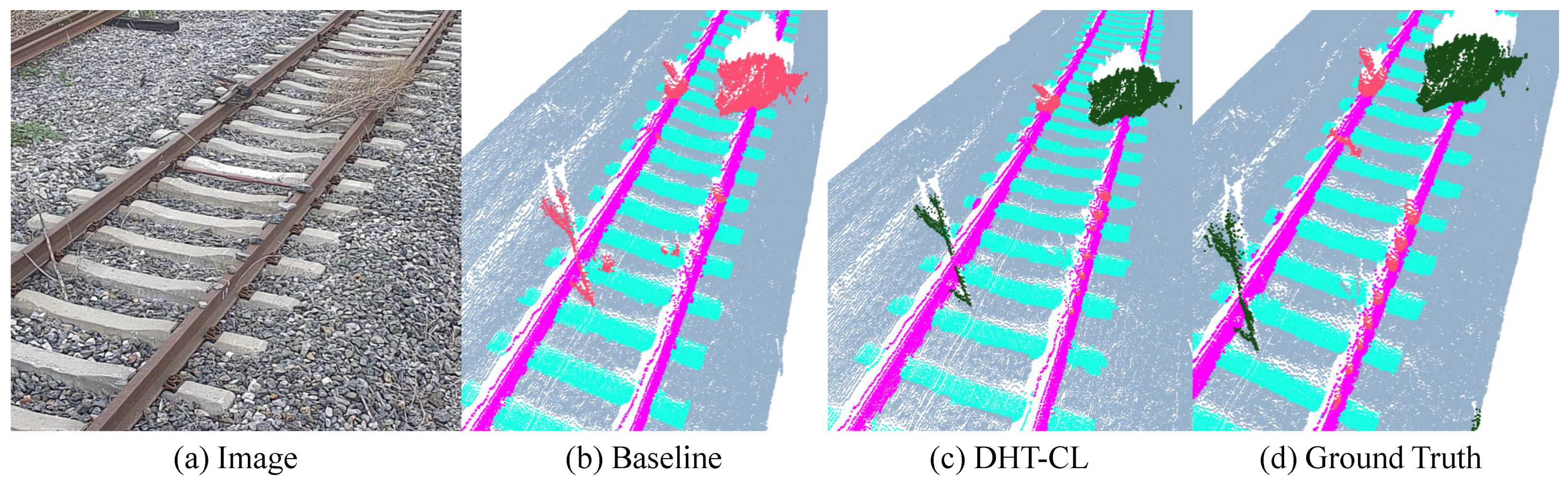
4.3.5. Visualization Results

Figure 11 shows the visualized segmentation results in clear weather. Enhanced by DHT-CL, the model acquired the color and geometric structure of the “plant” class and was able to distinguish it from the “unknown obstacle” class. There are eight stone obstacles visible in the bottom right of the image, ranging from large to small. The baseline model was able to identify three, whereas the enhanced model was able to identify seven.

Figure 12 shows the visualized segmentation results in rainy weather. The contour around the stone obstacle appears segmented more completely after enhancement by DHT-CL. In addition, the reflectivity contrast between the rail tracks, sleepers, and the gravel increased due to rain, and some of the sleepers were misclassified, resulting in false alarms, which were eliminated after the acquisition of color and neighborhood information through DHT-CL.

Figure 13 shows the segmentation results outside the overlapping FOV region of the LiDAR sensors and camera in rainy and snowy weather. The image on the left shows an irregular missing point cloud on a rainy day due to raindrop occlusion, with misidentification occurring near the missing portion. The image on the right shows a snowy day when objects around the tracks were incorrectly identified as a threat “plant” class due to snow accumulation. Classification confusion was eliminated through the use of DHT-CL. In short, the main effect of DHT-CL in rain and snow was to reduce the number of false-positive obstacle cases. In addition, the point clouds in the figure are outside the overlapping FOV region, and the method still yielded a performance enhancement, suggesting that the ability of the camera to access color information and the advantages of the two imaging perspectives have been internalized into the pure point cloud model.

4.3.6. Model Convergence

The mIoU and mAcc values obtained on the validation set, varying with the epoch, are shown in Figure 14. The curve shows that the model converged well during training up to 63 epochs. The two concave valleys in the mIoU–epoch curve (about the 9th and 30th epochs) come from restarting the learning rate. Our learning rate strategy is shown in Figure A4. The total losses, varying with the epoch on the validation set and the step on the training set, are shown in Figure 15 and Figure 16, respectively. Due to the large-scale absence of point clouds under rainy and snowy conditions, as shown in Figure A5, i.e., the presence of noise in the training data that was off-distribution, anomalous gradients were generated at certain steps, resulting in spiky noise in the training losses, but the overall tendency was to stabilize.

4.4. Rail-Obstacle Detection in Complex Weather

We further evaluated the performance of the rail-obstacle detection task in applications, and 1000 frames of data were selected for testing. In order to assess performance as comprehensively as possible, we compensated for the lower probability of rail obstacles in real-world environments by increasing the percentage of obstacle-containing frames in our tests, i.e., 411 (out of 1000) frames contained rail obstacles. The test data were collected under natural rainy and snowy conditions, and included multi-class rail obstacles, such as fallen trees, pedestrians, irregular stones, etc., with a minimum size of $7\times 7\times 7$ cm³ (which meets the Chinese rail-obstacle detection standard). Two metrics, i.e., the missed alarm ($MA$) rate and false alarm ($FA$) rate, were utilized for the performance evaluation. The formulations are as follows:

$$MA=\frac{FN}{TP+FN}$$

(15)

$$FA=\frac{FP}{TP+FP}$$

(16)

where $TP$ denotes true positive, i.e., the correctly predicted obstacle frames; $TN$ denotes true negative, i.e., the correctly predicted non-obstacle frames; $FP$ denotes false positive, i.e., the false obstacle frames; and $FN$ denotes false negative, i.e., the missed obstacle frames.

The results of rail-obstacle detection in complex weather are shown in

Table 5. Rail-obstacle detection results in complex weather.

	LiDAR Only	LiDAR + Camera
Missed alarm (MA) rate	1.72%	0.00%
False alarm (FA) rate	2.67%	0.48%

. Note that the $FA$ metric does not mean that 0.48% of the total number of tests will be false alarms but rather that the confidence level of the reported alarms is 99.52%. Overall, the experimental results show that the LiDAR + camera method, i.e., the DHT-CL model, significantly reduced the missed alarm and false alarm rates compared to the LiDAR-only method, i.e., the baseline model with point clouds only. The missed alarms in the LiDAR-only method were mostly caused by the inability to recognize small-sized obstacles, and the false alarms were mostly caused by confusion in segmentation due to changes in reflectivity on rainy and snowy days. The false alarms in the LiDAR + camera method were caused by extremely heavy rainfall, at which point the sensor was out of action, as shown in Figure A2. In addition, the detailed workflow of the algorithm for generating obstacle alarms is shown in Appendix B.

5. Conclusions

In this paper, a multi-modal contrast learning strategy, named DHT-CL, is proposed to enhance the performance of point cloud 3DSS in complex weather, improving the robustness of railway-obstacle detection in real-world scenarios. The contrast learning strategy is guided by a sliding kernel-based attention mechanism, which extracts neighborhood cross-modal information and exhibits superior performance in rainy and snowy conditions. An adaptive contrast learning strategy is developed for rail-obstacle detection, which can also be applied to more general scenarios with certain prior knowledge. The proposed DHT-CL strategy achieved an mIoU of 87.38% in full-scene segmentation of railway point clouds under complex weather conditions. In addition, it achieved a missed alarm rate of 0.00% and a false alarm rate of 0.48% in the rail-obstacle detection task under adverse weather conditions. Our future work will refine the functionality of the execution module, e.g., excluding false alarms through multi-frame voting and addressing dynamic scenes, and implement model compression suitable for the computational resources of mobile devices.

References

1. Zhangyu, W.; Guizhen, Y.; Xinkai, W.; Haoran, L.; Da, L. A Camera and LiDAR Data Fusion Method for Railway Object Detection. IEEE Sens. J. 2021, 21, 13442–13454. [Google Scholar] [CrossRef]
2. Soilán, M.; Nóvoa, A.; Sánchez-Rodríguez, A.; Riveiro, B.; Arias, P. Semantic Segmentaion of Point Clouds with PointNet AND KPConv Architectures Applied to Railway Tunnels. ISPRS Ann. Photogramm. Remote Sens. Spat. Inf. Sci. 2020, 2, 281–288. [Google Scholar] [CrossRef]
3. Manier, A.; Moras, J.; Michelin, J.C.; Piet-Lahanier, H. Railway Lidar Semantic Segmentation with Axially Symmetrical Convlutional Learning. ISPRS Ann. Photogramm. Remote Sens. Spat. Inf. Sci. 2022, 2, 135–142. [Google Scholar] [CrossRef]
4. Dibari, P.; Nitti, M.; Maglietta, R.; Castellano, G.; Dimauro, G.; Reno, V. Semantic Segmentation of Multimodal Point Clouds from the Railway Context. In Multimodal Sensing and Artificial Intelligence: Technologies and Applications II; Stella, E., Ed.; SPIE: Bellingham, WA, USA, 2021; Volume 11785. [Google Scholar] [CrossRef]
5. Le, M.H.; Cheng, C.H.; Liu, D.G. An Efficient Adaptive Noise Removal Filter on Range Images for LiDAR Point Clouds. Electronics 2023, 12, 2150. [Google Scholar] [CrossRef]
6. Le, M.H.; Cheng, C.H.; Liu, D.G.; Nguyen, T.T. An Adaptive Group of Density Outlier Removal Filter: Snow Particle Removal from LiDAR Data. Electronics 2022, 11, 2993. [Google Scholar] [CrossRef]
7. Wang, W.; You, X.; Chen, L.; Tian, J.; Tang, F.; Zhang, L. A Scalable and Accurate De-Snowing Algorithm for LiDAR Point Clouds in Winter. Remote Sens. 2022, 14, 1468. [Google Scholar] [CrossRef]
8. Mai, N.A.M.; Duthon, P.; Khoudour, L.; Crouzil, A.; Velastin, S.A. 3D Object Detection with SLS-Fusion Network in Foggy Weather Conditions. Sensors 2021, 21, 6711. [Google Scholar] [CrossRef] [PubMed]
9. Shih, Y.C.; Liao, W.H.; Lin, W.C.; Wong, S.K.; Wang, C.C. Reconstruction and Synthesis of Lidar Point Clouds of Spray. IEEE Robot. Autom. Lett. 2022, 7, 3765–3772. [Google Scholar] [CrossRef]
10. Boulch, A.; Guerry, J.; Le Saux, B.; Audebert, N. SnapNet: 3D point cloud semantic labeling with 2D deep segmentation networks. Comput. Graph. 2018, 71, 189–198. [Google Scholar] [CrossRef]
11. El Madawi, K.; Rashed, H.; El Sallab, A.; Nasr, O.; Kamel, H.; Yogamani, S. RGB and LiDAR fusion based 3D Semantic Segmentation for Autonomous Driving. In Proceedings of the 2019 IEEE Intelligent Transportation Systems Conference (ITSC), Auckland, New Zealand, 27–30 October 2019; pp. 7–12. [Google Scholar] [CrossRef]
12. Sun, Y.; Zuo, W.; Yun, P.; Wang, H.; Liu, M. FuseSeg: Semantic Segmentation of Urban Scenes Based on RGB and Thermal Data Fusion. IEEE Trans. Autom. Sci. Eng. 2021, 18, 1000–1011. [Google Scholar] [CrossRef]
13. Genova, K.; Yin, X.; Kundu, A.; Pantofaru, C.; Cole, F.; Sud, A.; Brewington, B.; Shucker, B.; Funkhouser, T. Learning 3D Semantic Segmentation with only 2D Image Supervision. In Proceedings of the 2021 International Conference on 3D Vision (3DV), London, UK, 1–3 December 2021; pp. 361–372. [Google Scholar] [CrossRef]
14. Vora, S.; Lang, A.H.; Helou, B.; Beijbom, O. PointPainting: Sequential Fusion for 3D Object Detection. In Proceedings of the 2020 IEEE/CVF Conference on Computer Vision and Pattern Recognition (CVPR), Seattle, WA, USA, 13–19 June 2020; pp. 4603–4611. [Google Scholar] [CrossRef]
15. Yang, Z.; Zhang, S.; Wang, L.; Luo, J. SAT: 2D Semantics Assisted Training for 3D Visual Grounding. In Proceedings of the 2021 IEEE/CVF International Conference on Computer Vision (ICCV), Montreal, QC, Canada, 10–17 October 2021; pp. 1836–1846. [Google Scholar] [CrossRef]
16. Zhuang, Z.; Li, R.; Jia, K.; Wang, Q.; Li, Y.; Tan, M. Perception-Aware Multi-Sensor Fusion for 3D LiDAR Semantic Segmentation. In Proceedings of the 2021 IEEE/CVF International Conference on Computer Vision (ICCV), Montreal, QC, Canada, 10–17 October 2021; pp. 16260–16270. [Google Scholar] [CrossRef]
17. Liu, Z.; Qi, X.; Fu, C.W. 3D-to-2D Distillation for Indoor Scene Parsing. In Proceedings of the 2021 IEEE/CVF Conference on Computer Vision and Pattern Recognition (CVPR), Nashville, TN, USA, 19–25 June 2021; pp. 4462–4472. [Google Scholar] [CrossRef]
18. Li, J.; Dai, H.; Han, H.; Ding, Y. MSeg3D: Multi-Modal 3D Semantic Segmentation for Autonomous Driving. In Proceedings of the 2023 IEEE/CVF Conference on Computer Vision and Pattern Recognition (CVPR), Vancouver, BC, Canada, 17–24 June 2023; pp. 21694–21704. [Google Scholar] [CrossRef]
19. Yan, X.; Gao, J.; Zheng, C.; Zheng, C.; Zhang, R.; Cui, S.; Li, Z. 2DPASS: 2D Priors Assisted Semantic Segmentation on LiDAR Point Clouds. arXiv 2022, arXiv:cs.CV/2207.04397. [Google Scholar]
20. Mahmoud, A.; Hu, J.S.K.; Kuai, T.; Harakeh, A.; Paull, L.; Waslander, S.L. Self-Supervised Image-to-Point Distillation via Semantically Tolerant Contrastive Loss. In Proceedings of the 2023 IEEE/CVF Conference on Computer Vision and Pattern Recognition (CVPR), Vancouver, BC, Canada, 17–24 June 2023; pp. 7102–7110. [Google Scholar] [CrossRef]
21. Hou, Y.; Zhu, X.; Ma, Y.; Loy, C.C.; Li, Y. Point-to-Voxel Knowledge Distillation for LiDAR Semantic Segmentation. In Proceedings of the 2022 IEEE/CVF Conference on Computer Vision and Pattern Recognition (CVPR), New Orleans, LA, USA, 18–24 June 2022; pp. 8469–8478. [Google Scholar] [CrossRef]
22. Zhou, H.; Zhu, X.; Song, X.; Ma, Y.; Wang, Z.; Li, H.; Lin, D. Cylinder3D: An Effective 3D Framework for Driving-scene LiDAR Semantic Segmentation. arXiv 2020, arXiv:cs.CV/2008.01550. [Google Scholar]
23. Liu, Z.; Tang, H.; Zhao, S.; Shao, K.; Han, S. PVNAS: 3D Neural Architecture Search With Point-Voxel Convolution. IEEE Trans. Pattern Anal. Mach. Intell. 2022, 44, 8552–8568. [Google Scholar] [CrossRef] [PubMed]
24. Choy, C.; Gwak, J.; Savarese, S. 4D Spatio-Temporal ConvNets: Minkowski Convolutional Neural Networks. In Proceedings of the 2019 IEEE/CVF Conference on Computer Vision and Pattern Recognition (CVPR), Long Beach, CA, USA, 15–20 June 2019; pp. 3070–3079. [Google Scholar] [CrossRef]
25. Behley, J.; Garbade, M.; Milioto, A.; Quenzel, J.; Behnke, S.; Stachniss, C.; Gall, J. SemanticKITTI: A Dataset for Semantic Scene Understanding of LiDAR Sequences. In Proceedings of the 2019 IEEE/CVF International Conference on Computer Vision (ICCV), Seoul, Republic of Korea, 27 October–2 November 2019; pp. 9296–9306. [Google Scholar] [CrossRef]
26. Xu, H.; Qiao, J.; Zhang, J.; Han, H.; Li, J.; Liu, L.; Wang, B. A High-Resolution Leaky Coaxial Cable Sensor Using a Wideband Chaotic Signal. Sensors 2018, 18, 4154. [Google Scholar] [CrossRef]
27. Catalano, A.; Bruno, F.A.; Galliano, C.; Pisco, M.; Persiano, G.V.; Cutolo, A.; Cusano, A. An optical fiber intrusion detection system for railway security. Sens. Actuators A Phys. 2017, 253, 91–100. [Google Scholar] [CrossRef]
28. SureshKumar, M.; Malar, G.P.P.; Harinisha, N.; Shanmugapriya, P. Railway Accident Prevention Using Ultrasonic Sensors. In Proceedings of the 2022 International Conference on Power, Energy, Control and Transmission Systems (ICPECTS), Chennai, India, 8–9 December 2022; pp. 1–5. [Google Scholar] [CrossRef]
29. Zhao, Y.; He, Y.; Que, Y.; Wang, Y. Millimeter wave radar denoising and obstacle detection in highly dynamic railway environment. In Proceedings of the 2023 IEEE 6th Information Technology, Networking, Electronic and Automation Control Conference (ITNEC), Chongqing, China, 24–26 February 2023; Volume 6, pp. 1149–1153. [Google Scholar] [CrossRef]
30. Gasparini, R.; D’Eusanio, A.; Borghi, G.; Pini, S.; Scaglione, G.; Calderara, S.; Fedeli, E.; Cucchiara, R. Anomaly Detection, Localization and Classification for Railway Inspection. In Proceedings of the 2020 25th International Conference on Pattern Recognition (ICPR), Milan, Italy, 10–15 January 2021; pp. 3419–3426. [Google Scholar] [CrossRef]
31. Fonseca Rodriguez, L.A.; Uribe, J.A.; Vargas Bonilla, J.F. Obstacle detection over rails using hough transform. In Proceedings of the 2012 XVII Symposium of Image, Signal Processing, and Artificial Vision (STSIVA), Medellin, Colombia, 12–14 September 2012; pp. 317–322. [Google Scholar] [CrossRef]
32. Uribe, J.A.; Fonseca, L.; Vargas, J.F. Video based system for railroad collision warning. In Proceedings of the 2012 IEEE International Carnahan Conference on Security Technology (ICCST), Newton, MA, USA, 15–18 October 2012; pp. 280–285. [Google Scholar] [CrossRef]
33. Kano, G.; Andrade, T.; Moutinho, A. Automatic Detection of Obstacles in Railway Tracks Using Monocular Camera. In Computer Vision Systems; Tzovaras, D., Giakoumis, D., Vincze, M., Argyros, A., Eds.; Springer: Cham, Switzerland, 2019; pp. 284–294. [Google Scholar]
34. Lu, J.; Xing, Y.; Lu, J. Intelligent Video Surveillance and Early Alarms Method for Railway Tunnel Collapse. In Proceedings of the 19th COTA International Conference of Transportation Professionals (CICTP 2019), Nanjing, China, 6–8 July 2019; pp. 1914–1925. [Google Scholar] [CrossRef]
35. Guan, L.; Jia, L.; Xie, Z.; Yin, C. A Lightweight Framework for Obstacle Detection in the Railway Image Based on Fast Region Proposal and Improved YOLO-Tiny Network. IEEE Trans. Instrum. Meas. 2022, 71, 1–16. [Google Scholar] [CrossRef]
36. Pan, H.; Li, Y.; Wang, H.; Tian, X. Railway Obstacle Intrusion Detection Based on Convolution Neural Network Multitask Learning. Electronics 2022, 11, 2697. [Google Scholar] [CrossRef]
37. Cao, Y.; Pan, H.; Wang, H.; Xu, X.; Li, Y.; Tian, Z.; Zhao, X. Small Object Detection Algorithm for Railway Scene. In Proceedings of the 2022 7th International Conference on Image, Vision and Computing (ICIVC), Xi’an, China, 26–28 July 2022; pp. 100–105. [Google Scholar] [CrossRef]
38. He, D.; Li, K.; Chen, Y.; Miao, J.; Li, X.; Shan, S.; Ren, R. Obstacle detection in dangerous railway track areas by a convolutional neural network. Meas. Sci. Technol. 2021, 32, 105401. [Google Scholar] [CrossRef]
39. Rampriya, R.S.; Suganya, R.; Nathan, S.; Perumal, P.S. A Comparative Assessment of Deep Neural Network Models for Detecting Obstacles in the Real Time Aerial Railway Track Images. Appl. Artif. Intell. 2022, 36, 2018184. [Google Scholar] [CrossRef]
40. Li, X.; Zhu, L.; Yu, Z.; Guo, B.; Wan, Y. Vanishing Point Detection and Rail Segmentation Based on Deep Multi-Task Learning. IEEE Access 2020, 8, 163015–163025. [Google Scholar] [CrossRef]
41. Šilar, Z.; Dobrovolný, M. The obstacle detection on the railway crossing based on optical flow and clustering. In Proceedings of the 2013 36th International Conference on Telecommunications and Signal Processing (TSP), Rome, Italy, 2–4 July 2013; pp. 755–759. [Google Scholar] [CrossRef]
42. Gong, T.; Zhu, L. Edge Intelligence-based Obstacle Intrusion Detection in Railway Transportation. In Proceedings of the GLOBECOM 2022—2022 IEEE Global Communications Conference (GLOBECOM), Rio de Janeiro, Brazil, 4–8 December 2022; pp. 2981–2986. [Google Scholar] [CrossRef]
43. Goodfellow, I.; Pouget-Abadie, J.; Mirza, M.; Xu, B.; Warde-Farley, D.; Ozair, S.; Courville, A.; Bengio, Y. Generative Adversarial Nets. In Proceedings of the Advances in Neural Information Processing Systems (NIPS), Montreal, QC, Canada, 8–13 December 2014; pp. 2672–2680. [Google Scholar]
44. Soilán, M.; Nóvoa, A.; Sánchez-Rodríguez, A.; Justo, A.; Riveiro, B. Fully automated methodology for the delineation of railway lanes and the generation of IFC alignment models using 3D point cloud data. Autom. Constr. 2021, 126, 103684. [Google Scholar] [CrossRef]
45. Sahebdivani, S.; Arefi, H.; Maboudi, M. Rail Track Detection and Projection-Based 3D Modeling from UAV Point Cloud. Sensors 2020, 20, 5220. [Google Scholar] [CrossRef] [PubMed]
46. Cserép, M.; Demján, A.; Mayer, F.; Tábori, B.; Hudoba, P. Effective railroad fragmentation and infrastructure recognition based on dense lidar point clouds. ISPRS Ann. Photogramm. Remote Sens. Spat. Inf. Sci. 2022, 2, 103–109. [Google Scholar] [CrossRef]
47. Karunathilake, A.; Honma, R.; Niina, Y. Self-Organized Model Fitting Method for Railway Structures Monitoring Using LiDAR Point Cloud. Remote Sens. 2020, 12, 3702. [Google Scholar] [CrossRef]
48. Han, F.; Liang, T.; Ren, J.; Li, Y. Automated Extraction of Rail Point Clouds by Multi-Scale Dimensional Features From MLS Data. IEEE Access 2023, 11, 32427–32436. [Google Scholar] [CrossRef]
49. Sánchez-Rodríguez, A.; Riveiro, B.; Soilán, M.; González-deSantos, L. Automated detection and decomposition of railway tunnels from Mobile Laser Scanning Datasets. Autom. Constr. 2018, 96, 171–179. [Google Scholar] [CrossRef]
50. Yu, X.; He, W.; Qian, X.; Yang, Y.; Zhang, T.; Ou, L. Real-time rail recognition based on 3D point clouds. Meas. Sci. Technol. 2022, 33, 105207. [Google Scholar] [CrossRef]
51. Wang, Z.; Yu, G.; Chen, P.; Zhou, B.; Yang, S. FarNet: An Attention-Aggregation Network for Long-Range Rail Track Point Cloud Segmentation. IEEE Trans. Intell. Transp. Syst. 2022, 23, 13118–13126. [Google Scholar] [CrossRef]
52. Qu, J.; Li, S.; Li, Y.; Liu, L. Research on Railway Obstacle Detection Method Based on Developed Euclidean Clustering. Electronics 2023, 12, 1175. [Google Scholar] [CrossRef]
53. Charles, R.Q.; Su, H.; Kaichun, M.; Guibas, L.J. PointNet: Deep Learning on Point Sets for 3D Classification and Segmentation. In Proceedings of the 2017 IEEE Conference on Computer Vision and Pattern Recognition (CVPR), Honolulu, HI, USA, 21–26 July 2017; pp. 77–85. [Google Scholar] [CrossRef]
54. Qi, C.R.; Yi, L.; Su, H.; Guibas, L.J. PointNet++: Deep Hierarchical Feature Learning on Point Sets in a Metric Space. In Proceedings of the 31st International Conference on Neural Information Processing Systems (NIPS), Long Beach, CA, USA, 4–9 December 2017; pp. 5105–5114. [Google Scholar]
55. Thomas, H.; Qi, C.R.; Deschaud, J.E.; Marcotegui, B.; Goulette, F.; Guibas, L. KPConv: Flexible and Deformable Convolution for Point Clouds. In Proceedings of the 2019 IEEE/CVF International Conference on Computer Vision (ICCV), Seoul, Republic of Korea, 27 October–2 November 2019; pp. 6410–6419. [Google Scholar] [CrossRef]
56. Hussain, M.; Ali, N.; Hong, J.E. DeepGuard: A framework for safeguarding autonomous driving systems from inconsistent behaviour. Autom. Softw. Eng. 2022, 29, 1. [Google Scholar] [CrossRef]
57. Liu, Z.; Cai, Y.; Wang, H.; Chen, L.; Gao, H.; Jia, Y.; Li, Y. Robust Target Recognition and Tracking of Self-Driving Cars With Radar and Camera Information Fusion Under Severe Weather Conditions. IEEE Trans. Intell. Transp. Syst. 2022, 23, 6640–6653. [Google Scholar] [CrossRef]
58. Stocco, A.; Tonella, P. Towards Anomaly Detectors that Learn Continuously. In Proceedings of the 2020 IEEE International Symposium on Software Reliability Engineering Workshops (ISSREW), Coimbra, Portugal, 12–15 October 2020; pp. 201–208. [Google Scholar] [CrossRef]
59. Alexiou, E.; Ebrahimi, T. Towards a Point Cloud Structural Similarity Metric. In Proceedings of the 2020 IEEE International Conference on Multimedia and Expo Workshops (ICMEW), London, UK, 6–10 July 2020; pp. 1–6. [Google Scholar] [CrossRef]
60. Meynet, G.; Nehmé, Y.; Digne, J.; Lavoué, G. PCQM: A Full-Reference Quality Metric for Colored 3D Point Clouds. In Proceedings of the 2020 Twelfth International Conference on Quality of Multimedia Experience (QoMEX), Athlone, Ireland, 26–28 May 2020; pp. 1–6. [Google Scholar] [CrossRef]
61. Meynet, G.; Digne, J.; Lavoué, G. PC-MSDM: A quality metric for 3D point clouds. In Proceedings of the 2019 Eleventh International Conference on Quality of Multimedia Experience (QoMEX), Berlin, Germany, 5–7 June 2019; pp. 1–3. [Google Scholar] [CrossRef]
62. Lu, Z.; Huang, H.; Zeng, H.; Hou, J.; Ma, K.K. Point Cloud Quality Assessment via 3D Edge Similarity Measurement. IEEE Signal Process. Lett. 2022, 29, 1804–1808. [Google Scholar] [CrossRef]
63. Zhang, Z.; Sun, W.; Min, X.; Wang, T.; Lu, W.; Zhai, G. No-Reference Quality Assessment for 3D Colored Point Cloud and Mesh Models. IEEE Trans. Circuits Syst. Video Technol. 2022, 32, 7618–7631. [Google Scholar] [CrossRef]
64. Liu, Q.; Yuan, H.; Su, H.; Liu, H.; Wang, Y.; Yang, H.; Hou, J. PQA-Net: Deep No Reference Point Cloud Quality Assessment via Multi-View Projection. IEEE Trans. Circuits Syst. Video Technol. 2021, 31, 4645–4660. [Google Scholar] [CrossRef]
65. Viola, I.; Cesar, P. A Reduced Reference Metric for Visual Quality Evaluation of Point Cloud Contents. IEEE Signal Process. Lett. 2020, 27, 1660–1664. [Google Scholar] [CrossRef]
66. Zhou, W.; Yue, G.; Zhang, R.; Qin, Y.; Liu, H. Reduced-Reference Quality Assessment of Point Clouds via Content-Oriented Saliency Projection. IEEE Signal Process. Lett. 2023, 30, 354–358. [Google Scholar] [CrossRef]
67. Kim, J.; Park, B.j.; Kim, J. Empirical Analysis of Autonomous Vehicle’s LiDAR Detection Performance Degradation for Actual Road Driving in Rain and Fog. Sensors 2023, 23, 2972. [Google Scholar] [CrossRef]
68. Montalban, K.; Reymann, C.; Atchuthan, D.; Dupouy, P.E.; Riviere, N.; Lacroix, S. A Quantitative Analysis of Point Clouds from Automotive Lidars Exposed to Artificial Rain and Fog. Atmosphere 2021, 12, 738. [Google Scholar] [CrossRef]
69. Piroli, A.; Dallabetta, V.; Kopp, J.; Walessa, M.; Meissner, D.; Dietmayer, K. Energy-Based Detection of Adverse Weather Effects in LiDAR Data. IEEE Robot. Autom. Lett. 2023, 8, 4322–4329. [Google Scholar] [CrossRef]
70. Li, Y.; Duthon, P.; Colomb, M.; Ibanez-Guzman, J. What Happens for a ToF LiDAR in Fog? IEEE Trans. Intell. Transp. Syst. 2021, 22, 6670–6681. [Google Scholar] [CrossRef]
71. Delecki, H.; Itkina, M.; Lange, B.; Senanayake, R.; Kochenderfer, M.J. How Do We Fail? Stress Testing Perception in Autonomous Vehicles. In Proceedings of the 2022 IEEE/RSJ International Conference on Intelligent Robots and Systems (IROS), Kyoto, Japan, 23–27 October 2022; pp. 5139–5146. [Google Scholar] [CrossRef]
72. Hinton, G.E.; Vinyals, O.; Dean, J. Distilling the Knowledge in a Neural Network. arXiv 2015, arXiv:abs/1503.02531. [Google Scholar]
73. He, K.; Zhang, X.; Ren, S.; Sun, J. Deep Residual Learning for Image Recognition. In Proceedings of the 2016 IEEE Conference on Computer Vision and Pattern Recognition (CVPR), Las Vegas, NV, USA, 27–30 June 2016; pp. 770–778. [Google Scholar] [CrossRef]
74. Zhang, Z. A flexible new technique for camera calibration. IEEE Trans. Pattern Anal. Mach. Intell. 2000, 22, 1330–1334. [Google Scholar] [CrossRef]
75. Yuan, C.; Liu, X.; Hong, X.; Zhang, F. Pixel-Level Extrinsic Self Calibration of High Resolution LiDAR and Camera in Targetless Environments. IEEE Robot. Autom. Lett. 2021, 6, 7517–7524. [Google Scholar] [CrossRef]
76. Jaritz, M.; Vu, T.H.; de Charette, R.; Wirbel, E.; Pérez, P. xMUDA: Cross-Modal Unsupervised Domain Adaptation for 3D Semantic Segmentation. In Proceedings of the 2020 IEEE/CVF Conference on Computer Vision and Pattern Recognition (CVPR), Seattle, WA, USA, 13–19 June 2020; pp. 12602–12611. [Google Scholar] [CrossRef]
77. Xiong, R.; Yang, Y.; He, D.; Zheng, K.; Zheng, S.; Xing, C.; Zhang, H.; Lan, Y.; Wang, L.; Liu, T.Y. On Layer Normalization in the Transformer Architecture. arXiv 2020, arXiv:cs.LG/2002.04745. [Google Scholar]
78. Graham, B.; Engelcke, M.; Maaten, L.v.d. 3D Semantic Segmentation with Submanifold Sparse Convolutional Networks. In Proceedings of the 2018 IEEE/CVF Conference on Computer Vision and Pattern Recognition, Salt Lake City, UT, USA, 18–22 June 2018; pp. 9224–9232. [Google Scholar] [CrossRef]
79. Yan, Y.; Mao, Y.; Li, B. SECOND: Sparsely Embedded Convolutional Detection. Sensors 2018, 18, 3337. [Google Scholar] [CrossRef]
80. Wang, F.; Liu, H. Understanding the Behaviour of Contrastive Loss. In Proceedings of the 2021 IEEE/CVF Conference on Computer Vision and Pattern Recognition (CVPR), Nashville, TN, USA, 19–25 June 2021; pp. 2495–2504. [Google Scholar] [CrossRef]
81. Berman, M.; Triki, A.R.; Blaschko, M.B. The Lovasz-Softmax Loss: A Tractable Surrogate for the Optimization of the Intersection-Over-Union Measure in Neural Networks. In Proceedings of the 2018 IEEE/CVF Conference on Computer Vision and Pattern Recognition, Salt Lake City, UT, USA, 18–22 June 2018; pp. 4413–4421. [Google Scholar] [CrossRef]
Figure 1. Railway point clouds in sunny and rainy weather. The top is sunny and the bottom is rainy. The point clouds are coloured by light intensity (strong to weak corresponds to red to blue).
Electronics 13 00220 g001
Figure 2. Distribution of railway point cloud intensity under different weather conditions.
Electronics 13 00220 g002
Figure 3. Receptive fields of 2D and 3D networks: (a) 2D network receptive field, (b) projecting the point cloud onto the image, (c) re-projecting the 2D network receptive field into 3D, (d) 3D network receptive field. The re-projected 2D receptive field does not coincide with the 3D receptive field. Orange indicates receptive fields and blue indicates background.
Electronics 13 00220 g003
Figure 4. Overview of DHT-CL. The point clouds and the images are processed independently by 2D and 3D encoding networks to generate the corresponding 2D and 3D features. Then, the DHT module extracts deeper information from these features, delivering the fusion features. Modality-independent classifiers generate two prediction scores, upon which the obstacle anomaly-aware modality discrimination loss is constructed. All processes are supervised by 3D labels, with only the 3D branch activated during the inference stage. Raw point clouds are coloured by intensity and labels are coloured by different object classes.
Electronics 13 00220 g004
Figure 5. Framework of the DHT module. Cross-attention is applied twice to the 2D and pseudo-2D features.
Electronics 13 00220 g005
Figure 6. Schematic diagram of the local attention mechanism within the DHT module. (a) Selection of an anchor point, represented as a query vector Q (in red). (b) Search for neighborhood points (in blue) around this anchor point within a sliding window (a 5 × 5 kernel is shown in this diagram). Note that neighborhood points may be missing due to the sparsity of the point cloud. The missing points are indicated in gray. (c) Omission of the missing points by marking them as −1 in the GPU Hash table-based neighborhood address query operation. (d) Flattening of the irregular matrix and utilization as a key vector. Then, computing of the inner product between the query vector Q (in red) and the key vector K (in blue) to derive the attention weights. (e) Adjusting weight K by applying the weights derived from Q K T . (f) Updating the center element of the sliding window to produce the final output.
Electronics 13 00220 g006
Figure 7. Schematic diagram of adaptive contrastive learning strategy.
Electronics 13 00220 g007
Figure 8. Railway monitoring equipment.
Electronics 13 00220 g008
Figure 9. Label distribution of proposed complex weather railway dataset.
Electronics 13 00220 g009
Figure 10. mIoU and mAcc at different distances and point cloud densities.
Electronics 13 00220 g010
Figure 11. The segmentation results of DHT-CL in clear weather. Colour meanings are as follows: purple: rail track, light blue: sleeper, cyan: gravel bed, green: plant, salmon red: unknown obstacle.
Electronics 13 00220 g011
Figure 12. The segmentation results of DHT-CL in rainy weather: (a) Image in rain. (b) Pure 3D net baseline without DHT-CL. (c) Enhanced by DHT-CL. (d) Ground-truth labels.
Electronics 13 00220 g012
Figure 13. The segmentation results of DHT-CL outside the FOVs in rainy and snowy weather: (a) Pure 3D net baseline without DHT-CL. (b) Enhanced by DHT-CL. (c) Ground-truth labels. Left is raining and right is snowing.
Electronics 13 00220 g013
Figure 14. mIoU and mAcc values on the validation set, varying with the epoch.
Electronics 13 00220 g014
Figure 15. Total loss per epoch.
Electronics 13 00220 g015
Figure 16. Total loss per step.
Electronics 13 00220 g016