3.1. Low-Light Image Training Datasets
Existing large-scale genera-purpose target recognition datasets contain only a very small number of low-light image samples, e.g., Microsoft COCO [
19], ImageNet [
20], and PASCAL VOC [
21], whose low-light images account for only about 1% of all samples, making it difficult to use them effectively for training low-light image recognition models. Therefore, the public dataset ExDark [
22], which consists of all low-light images with target-level annotations, is selected as the base dataset in this paper. The ExDark dataset contains 7363 low-light images with 12 different target classes. Among them, the training set contains 3000 images with 250 images in each category, the validation set contains 1800 images with 150 images in each category, and the test set contains 2563 images. Most of the images in the dataset were downloaded from search engines, and a few images were selected from the large public datasets mentioned above (Microsoft COCO, etc.). The resolution and aspect ratios of these images vary widely, and the quality of the images captured is variable. In addition to the target types, ExDark includes information on 10 different low-light scene categories, ranging from very low light to low light for complex low-light scenes. It is worth noting that the dataset does not contain normal exposure images paired with low-light images, making it difficult to apply supervised low-light image enhancement algorithms to them.
The ExDark dataset contains a wide variety of scenes covering common low-light scene types: (a) very low-light images; (b) low-light images with no light source; (c) low-light images with an illuminated object surrounded by darkness; (d) low-light images with a single visible light source; (e) low-light images with multiple, but weaker light sources; (f) low-light images with multiple, but stronger light sources; (g) low-light images with visible screens; (h) low-light images of an interior room with brightly lit windows; (i) low-light images of an interior room with brightly lit screens; (j) low-light images of an interior room; (k) low-light images of a target to be inspected in shadow; (l) low-light images of a target to be inspected in darkness; and (m) low-light images of a target to be inspected in a dark room with bright windows. The complexity of the scene types contained in this dataset greatly increases the difficulty of recognition and detection, and it is difficult for unimproved general-purpose target detection methods to work well enough on this dataset. At the same time, the ExDark training dataset is too small, which affects the performance of the model, so there is a great need to expand the ExDark dataset to improve the generalization ability of the model.
This section may be divided by subheadings. It should provide a concise and precise description of the experimental results, their interpretation, as well as the experimental conclusions that can be drawn.
3.2. Low-Level Image Enhancement
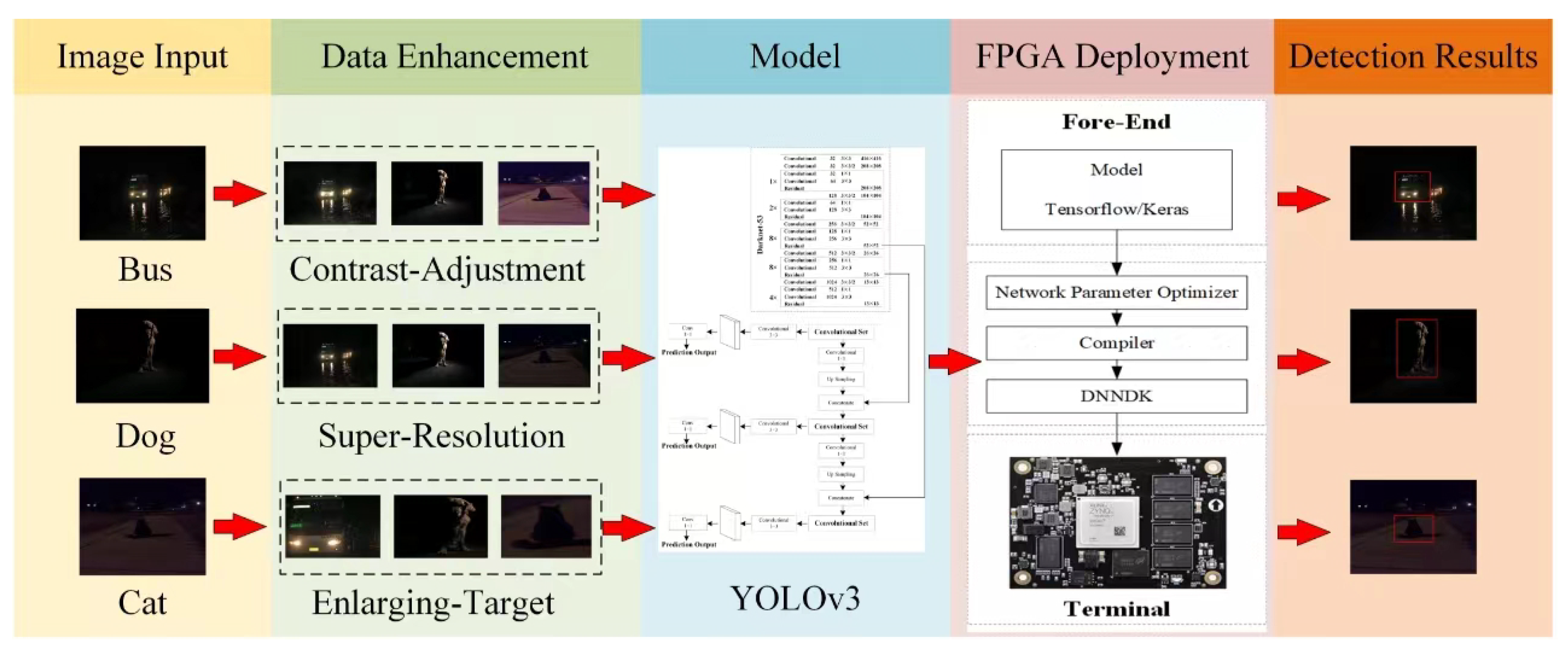
Most of the current publicly available low-light image datasets are from the image enhancement domain, where the images have no detection annotation information and the number of them is difficult to support the training of shimmering image detection models. In order to increase the available datasets, we will expand the datasets by collecting 5000 low-light images from the real world and generate more low-light images by combining low-order image enhancement techniques. Three low-cost image enhancement methods will be used to process the ExDark and reality images, namely contrast adjustment, enlarging target, and super resolution.
Contrast Adjustment: In this paper, the Histogram Equalization (HE) method is used to adjust the contrast of an image. This method makes the distribution of grey levels in the histogram more uniform, so that the dynamic range is expanded, thus enhancing the contrast of the whole image [
23].
Assuming that the grey level distribution of the very first image is
f,
g represents the grey level distribution of the original image after the HE method. Let the grey levels in the grey level distribution be
r and
s, and their corresponding numbers of pixels be
and
, respectively. Then the probability of the grey level distribution is given by Equation (
1), and
D stands for the total grey levels.
Equation (
2) is derived from Equation (
1):
In order to make the histogram uniformly distributed, it is necessary to make the distribution probability of each grey level equal, and the derivation yields Equation (
3):
Bringing Equation (
3) into Equation (
2) leads to Equation (
4):
This gives the transformation Equation (
5) for the HE method, where
is the distribution of the original map.
Enlarging Target: To better extract the subject features in low-light images, we use a modified seam carving algorithm to magnify the subject. The seam carving algorithm’s main feature is that it takes into account the importance of the content of the image, which defines the importance of the different scenes in the image through the energy function [
24]; then, by constantly deleting or copying the pixel lines that have the lowest energy, at the same time, it maintains the original appearance of the visual subject at the maximum extent. The original appearance of the visual subject at the same time accomplishes a non-equal aspect ratio zoom.
Let
i be an
image with vertical pixel lines defined as follows:
Here,
is the mapping:
. From the above equation, it can be seen that the vertical pixel line is an 8-connected path consisting of pixels from the first to the last row of the image, with one and only one pixel removed from each row. Similarly, the horizontal pixel line is defined as:
where
is the mapping:
. Horizontal pixel lines are 8-connected paths consisting of pixels from the first to the last column of the image, with one and only one pixel removed from each column. Thus, the path of the vertical pixel line is
. Then the path of the horizontal pixel line has a similar situation. If a row or column of an image is to be deleted, then processing an image results in all pixels below or to the right of the line being shifted up or to the left to complement the deleted pixel line.
Line cropping has a limited effect on the visual appearance of an image; it only affects the area around the line being deleted or added, and has no effect at all on the remaining pixels in the image. Therefore, it is crucial to find the appropriate pixel line. Knowing that the energy function of each pixel of an image is
e, the total energy of the pixel line is defined as
Find the vertical pixel line with the lowest total energy:
The horizontal pixel lines are found in a similar way. The finding of the lowest energy pixel line is solved using the dynamic programming method. For a pixel point
in image
I, remembering that the cumulative energy of the point is
, we have
Therefore, it is only necessary to traverse the second to last row in image I and calculate the above equation to derive the cumulative energy. The pixel point in the last row with the smallest cumulative energy is the end point of the vertical pixel line with the smallest energy. Then, we go back from this point, each time looking for the pixel point with the smallest cumulative energy in the field previous to the known minimum cumulative energy point, and so on, until the vertical pixel line with the smallest energy is found.
For finding horizontal pixel lines, the method is similar and has cumulative energy
, as in the following equation:
As can be seen from the formula for cumulative energy, the minimum of the last line of M must be the end of the vertical minimum energy line, so the vertical minimum energy line can be found by backtracking from this point. The method of finding the horizontal minimum energy line is similar.
To make the pixel importance calculation more reasonable, the original algorithm is improved by the following process: multiplying the gradient map with the visual saliency map to obtain the final importance energy map of the whole image, calculating the cumulative energy map of the image, and then searching for the lowest energy point, going back to find the lowest energy line, and deleting or inserting the lowest energy line to obtain the final target image. The improved algorithm can better preserve the subject effect, especially for visual subjects in dark lighting conditions.
Super Resolution: In this paper, we use the SwinIR network model based on Transformer to reconstruct the image with ultra-high resolution, which consists of three modules: shallow feature extraction, deep feature extraction, and reconstruction module [
25]. The shallow feature extraction module uses a convolutional layer to extract shallow features, which are passed directly to the reconstruction module to preserve low-frequency information. The deep feature extraction module consists mainly of residual Swin Transformer Blocks (RSTBs) containing Swin Transformers, and each RSTB uses multiple Swin Transformer layers for local attention and cross-window interaction. In addition, SwinIR adds a convolutional layer at the end of the block for feature enhancement and uses a residual link to provide a shortcut for feature aggregation. Finally, shallow and deep features are fused in the reconstruction module to achieve high-quality image reconstruction. The Swin Transformer layer is based on the standard multi-head self-attention of the original Transformer layer. The main difference is the self-attention and shift window mechanism. Given an input of size
, the Swin Transformer first transforms the input to
and divides it into one window with dimensions
and without overlapping, where
is the total number of windows. Then, the self-attention of each window is calculated separately. For a local window feature
, the query vector
Q, the key vector
K, and the value vector
V are computed as follows (12):
where
,
, and
are the learnable matrices of the query vectors, the key vectors, the value vectors, and share weights between the windows, respectively, and in general,
through the self-attention mechanism within a local window is calculated as can be seen below. The attention matrix is shown in Equation (
13):
where
B is the learnable relative positional encoding.
, and
represents the amount of attention from multiple heads. Thereafter, we execute the attention function
h times in parallel and stitch together the results of the multi-headed self-attention mechanism.
A multi-layer perception containing two fully connected layers is then used, with a Gelu nonlinear function between the fully connected layers, which increases the nonlinear expressiveness of the model. In addition, the multi-head attention using residual connections and the multi-layer LayerNorm layer is added before the two modules of multi-head attention and multi-layer perception using residual connection. The whole process is expressed in Equations (
14) and (
15):
In summary, we augmented the images using three lower-order image processing techniques with the aim of expanding the training dataset to improve the performance of the higher-order visual model, and
Figure 2 shows some of the processed images.


