MSGL+: Fast and Reliable Model Selection-Inspired Graph Metric Learning ^†

Abstract

The problem of learning graph-based data structures from data has attracted considerable attention in the past decade. Different types of data can be used to infer the graph structure, such as graphical Lasso, which is learned from multiple graph signals or graph metric learning based on node features. However, most existing methods that use node features to learn the graph face difficulties when the label signals of the data are incomplete. In particular, the pair-wise distance metric learning problem becomes intractable as the dimensionality of the node features increases. To address this challenge, we propose a novel method called MSGL+. MSGL+ is inspired from model selection, leverages recent advancements in graph spectral signal processing (GSP), and offers several key innovations: (1) Polynomial Interpretation: We use a polynomial function of a certain order on the graph Laplacian to represent the inverse covariance matrix of the graph nodes to rigorously formulate an optimization problem. (2) Convex Formulation: We formulate a convex optimization objective with a cone constraint that optimizes the coefficients of the polynomial, which makes our approach efficient. (3) Linear Constraints: We convert the cone constraint of the objective to a set of linear ones to further ensure the efficiency of our method. (4) Optimization Objective: We explore the properties of these linear constraints within the optimization objective, avoiding sub-optimal results by the removal of the box constraints on the optimization variables, and successfully further reduce the number of variables compared to our preliminary work, MSGL. (5) Efficient Solution: We solve the objective using the efficient linear-program-based Frank–Wolfe algorithm. Application examples, including binary classification, multi-class classification, binary image denoising, and time-series analysis, demonstrate that MSGL+ achieves competitive accuracy performance with a significant speed advantage compared to existing graphical Lasso and feature-based graph learning methods.

1. Introduction

Graph learning has been the subject of extensive research for over a decade. In recent years, there has been a growing convergence between machine learning [1] and graph signal processing in the spectral domain (GSP) [2,3,4,5]. These interdisciplinary efforts have led to applications in diverse domains, including data classification [6], social network management [2], image quality assessment [7], image enhancement [4], and clustering [8]. GSP primarily deals with signals defined on graphs, where vertices represent data points and weighted edges capture observation pair similarities. The central challenge in GSP combined with machine learning lies in designing graphs that effectively capture relationships among data observations. To achieve this, a signal prior—such as the concept of graph signal smoothness (GSS)—is formulated. On the other hand, another popular signal prior is graph total variation, which is generally more suitable for signals that are locally smooth or piecewise constant [9,10]. This prior facilitates efficient filtering of globally smooth graph signals [11,12], enabling tasks like data classification through extrapolation of the signal or propagation of the data label [13].

Graph structures can be acquired in two ways: (1) raw data collection, e.g., time-series data [14]; (2) constructed features derived from data samples. Given that successful graph filtering hinges on the effectiveness of the graph models and the structure of the data, graph learning assumes fundamental importance. Approaches to graph learning fall into two main tracks: (1) Data-focused graph learning: This approach learns the graph directly from raw data [15]. (2) Feature-based graph learning: Here, constructed features guide the graph learning process [16,17]. The data-focused graph learning track aims to model the relationships among multiple observations (graph signals) on graph nodes, which can be spatial and/or temporal. The authors of [14,15] used a Gaussian process with a GSS prior to learn the graph structure that corresponds to the graph Laplacian matrix $\mathbf{L}$ from M-dimensional observations on N nodes, $\mathbf{X}\in {\mathbb{R}}^{M\times N}$. The GSS prior was expressed by the quadratic form $\mathrm{Tr}\left({\mathbf{X}}^{\top }\mathbf{L}\mathbf{X}\right)$. A recent work [18] proposed a generalized smoothness prior of graph signals based on a quadratic function of a graph spectral kernel, which aims to optimize the spectrum of $\mathbf{L}$ via a polynomial function. In contrast, the feature-based graph learning track learns the feature graph structure constructed by a pre-defined or optimized metric function that measures feature relevance [17]. These methods simplify the problem by optimizing the metric function with a GSS prior of the form ${\mathbf{y}}^{\top }\mathbf{L}\mathbf{y}$, where $\mathbf{y}\in {\mathbb{R}}^N$ is a graph signal representing the labels of the samples, each assigned to one graph node. Similarly, [19] introduced a semi-supervised learning framework with a high-order regularizer ${\mathbf{y}}^{\top }{\mathbf{L}}^P\mathbf{y}$ (P denotes 1-to-P-hop neighbor) as the graph signal prior. For a graph-based classification task, an iterative process is generally applied by alternately learning an aforementioned graph structure that fits the data and a graph-based classifier [16,20,21,22,23,24,25], where the output of the iterative process is the predicted data labels.

Existing graph learning methods exhibit two primary approaches. The first approach involves solving systems of linear equations to update each graph node, exemplified by techniques like graphical Lasso [15], sparse graph learning [26,27], and learning of the low-dimensional space [28]. The second approach employs gradient descent to learn a pair-wise distance metric, as seen in methods such as distance metric learning [29] and feature graph learning [30]. However, both approaches suffer from scalability issues, as the number of optimization variables grows significantly with the number of data samples or feature dimensions. In our preliminary work [31], we address this limitation by introducing a novel method called Model Selection-Inspired Graph Learning (MSGL). MSGL leverages the signal prior enriched by data-focused graph learning methods within a model selection framework [18]. In this paper, we propose MSGL+, an improved graph learning method based on our previous work, MSGL [31]. Specifically, instead of using the conventional GSS prior, we use a signal prior defined on a graph spectral kernel, denoted as $\mathcal{L}={\sum }_{i=1}^P{\beta }_i{\mathbf{L}}^i$, where $\mathbf{L}$ represents the Laplacian matrix computed from data features. The kernel parameters $\mathit{\beta }$ play a crucial role in shaping the signal prior. To optimize $\mathit{\beta }$, we reinterpret $\mathcal{L}$ as a precision matrix [32] for single-observation data [17]. We formulate a convex optimization problem that ensures the positive definiteness of $\mathcal{L}$. By imposing a set of linear constraints on $\mathit{\beta }$, we enable efficient solution using the Frank–Wolfe method [33]. The main novelties and advantages of MSGL+ are summarized as follows:

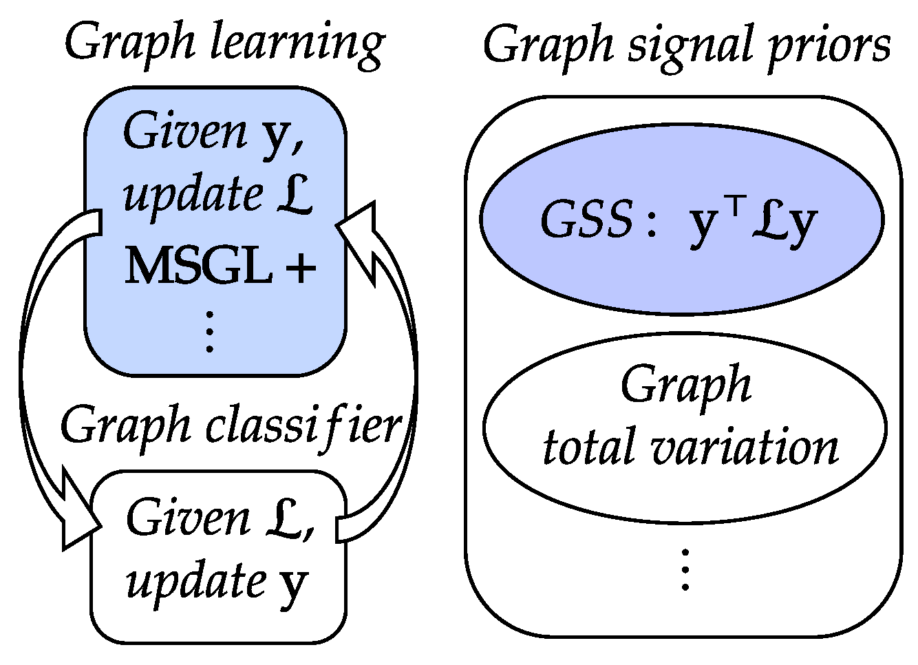
• In Equation (4), we introduce a novel graph learning framework that integrates graph kernel learning and graph signal processing. We achieve this by learning the coefficients of a polynomial kernel function that penalizes the signal’s Fourier coefficients with ${\sum }_{i=1}^P{\beta }_i{\lambda }_k^i+\mu$, where ${\lambda }_k$ are the eigenvalues of the graph Laplacian ${\mathbf{L}}_n$ and $\mathit{\beta }$ are the learnable parameters. This can be regarded as a generalization of the conventional smoothness prior ${\mathbf{y}}^{\top }{\mathbf{L}}_n\mathbf{y}$, which uses a fixed coefficient for all eigenvalues.
• In Algorithm 1 in Section 1, we formulate the graph learning problem as a convex optimization objective that consists of a GSS prior with $\mathcal{L}$ and a model complexity penalty with ${\mathcal{L}}^{-1}$. We convert the positive definite constraint for $\mathcal{L}$ into a group of linear constraints for $\mathit{\beta }$. We then solve the problem efficiently using the Frank–Wolfe method, which only requires linear programs at each iteration.

  Algorithm 1 The proposed MSGL+ graph metric learning method.

  Input: $\mathcal{D}={\left\{({\mathbf{f}}_i,y_i)\right\}}_{i=1}^N$, $\mu$, P.

  Output: ${\mathit{\beta }}^{*}$.

  1: Construct $\mathbf{L}$ using $\mathbf{f}$ via Equations (1) and (2). 2: Obtain eigenpairs $\mathbf{U}$ and ${\lambda }_1,...,{\lambda }_N$ of $\mathbf{L}$ via eigen decomposition. 3: Construct $\mathcal{L}$ with $\mathbf{U}$, ${\lambda }_1,...,{\lambda }_N$, $\mu$, P, and randomly initialized $\mathit{\beta }$ via Equation (4). 4: while not converged do: 5:      Solve Equation (25) for ${\mathbf{s}}^t$ via interior-point. 6:          while not converged do: 7:              Solve Equation (26) for ${\alpha }^t$ via a Newton–Raphson method. 8:          end while 9:          ${\mathit{\beta }}^t={\mathit{\beta }}^{t-1}+{\alpha }^t({\mathbf{s}}^t-{\mathit{\beta }}^{t-1}),\forall i\in 1,...,P-1$. 10: end while 11: Compute ${\beta }_P$ via Equation (7).

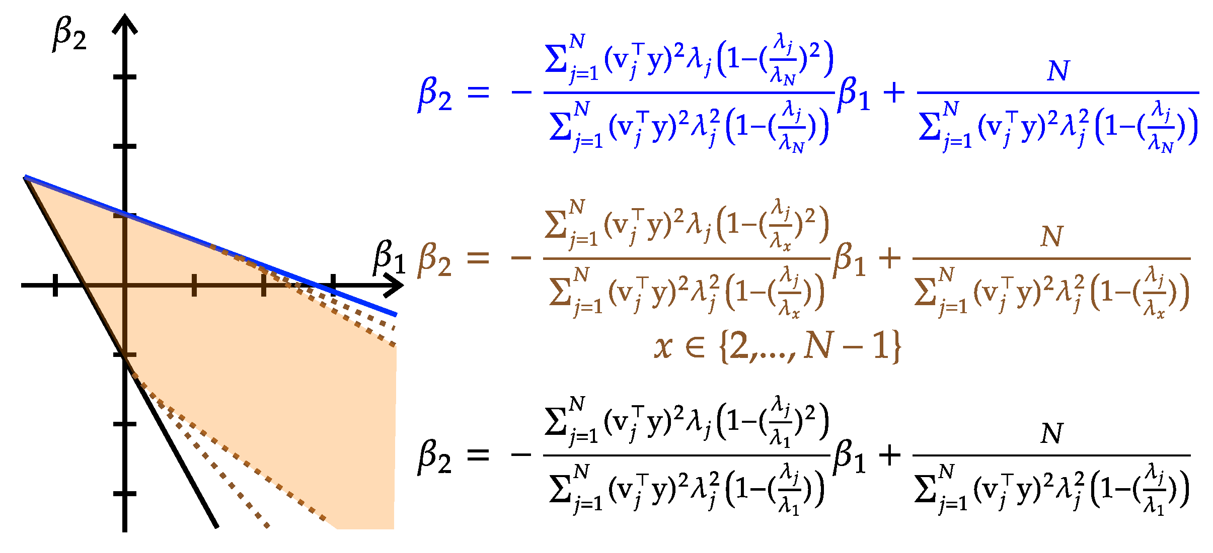
• In Equation (6) to Equation (28), we analyze the properties of the linear constraints and show that they ensure the positive definiteness of $\mathcal{L}$ without requiring any box constraints on $\mathit{\beta }$. We also show that we can reduce the number of optimization variables by exploring the properties of the linear constraints within the optimization objective, which leads to faster and more stable implementations than MSGL.
• In Section 3, we extend the applicability of MSGL+ to both metric matrix-defined feature-based positive graphs and graphical Lasso-learned signed graphs, which are two common types of graphs used in various applications. This extension from [31] significantly broadens the scope of MSGL+, as it can handle any symmetric, positive (semi-)definite matrix that corresponds to a (un)signed graph and learn the polynomial kernel coefficients via MSGL+.
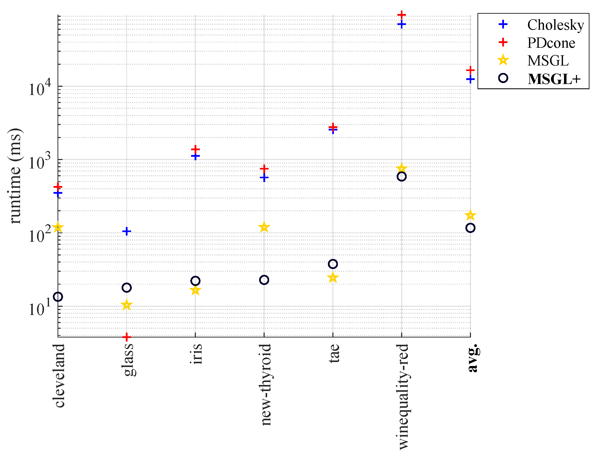
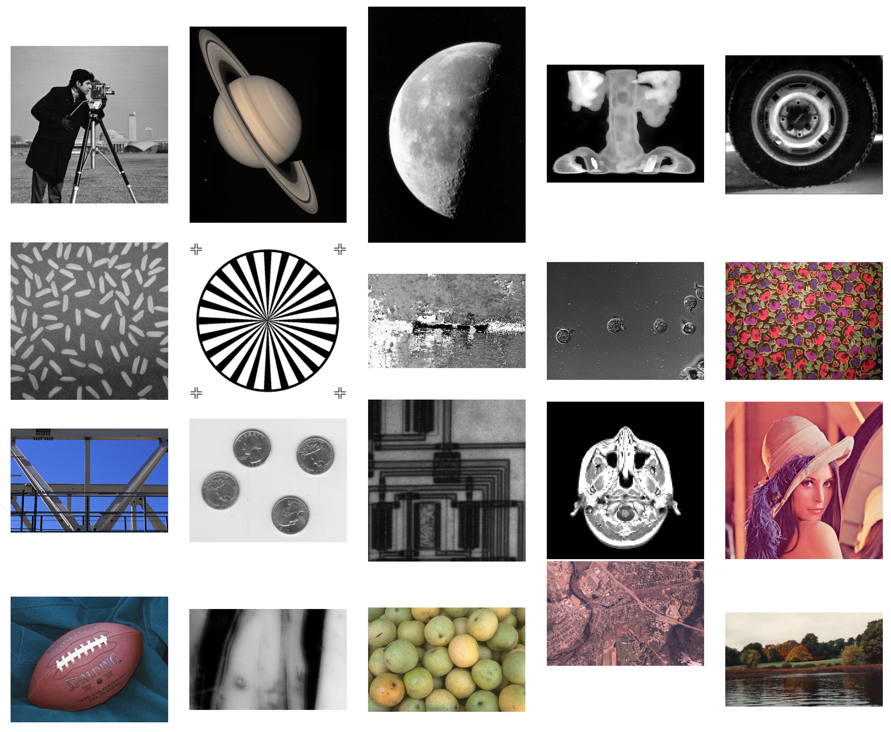
• In Section 3, we evaluate the performance of MSGL+ on various tasks, such as binary classification, multi-class classification, binary image denoising, and time-series analysis. We compare MSGL+ with several state-of-the-art graph learning methods and show that MSGL+ achieves comparable accuracy with much faster runtime.

See Figure 1 for an illustration of the relationship among graph learning (including our proposed MSGL+), graph classifiers, and graph signal priors in the context of graph-based classification. Our proposed MSGL+ method is more flexible than [17], which only optimizes the distances between sample pairs based on a predefined graph kernel $\mathbf{L}$. Instead, MSGL+ learns the optimal $\mathit{\beta }$ via a polynomial function $\mathcal{L}\left(\mathit{\beta }\right)$ with $\mathbf{L}$. Furthermore, we distinguish our method from [18] by tuning the precision matrix using a feature graph, rather than predicting the data using multi-dimensional raw data samples. Therefore, MSGL+ focuses on the kernel that is defined on the features corresponding to the training data in the input space, instead of the ones corresponding to the full data samples [18]. This essential difference results in MSGL+ being highly efficient during optimization given the one-time full eigen decomposition of $\mathbf{L}$, while [18] requires iterative eigenvalue or Cholesky decomposition during the entire optimization process. We demonstrate the effectiveness and efficiency of our proposed MSGL+ method through various applications, such as binary classification, multi-classification, binary image denoising, and time-series analysis, and compare it with existing graphical Lasso and feature-based graph learning methods.

The rest of the paper is structured as follows. We review the basic GSP tools in Section 2.1, formulate a convex optimization problem for our proposed MSGL+ graph learning method in Section 2.2, develop a fast and reliable algorithm that solves the convex optimization problem in Section 2.3, evaluate our proposed MSGL+ method via binary classification, multi-class classification, binary image denoising, and time-series analysis tasks and show our experimental results in Section 3, and discuss the experimental methods in Section 4. We conclude this paper in Section 5.

2. Materials and Methods

2.1. Preliminaries

We first define $\mathcal{G}$ as an undirected graph, specifically, $\mathcal{G}(\mathcal{V},\mathcal{E},\mathbf{A})$, where $\left|\mathcal{V}\right|=N$ denotes the number of nodes within the graph, $(i,j)\in \mathcal{E}$ denotes the edges within the graph, and $\mathbf{A}$ denotes the adjacency matrix whose entries $A_{ij}\in [0,+\infty )$ are non-negative edge weights defined with a Gaussian kernel:

$$\begin{array}{c}\hfill A_{ij}=\left\{\begin{array}{cc}exp\left\{-{({\mathbf{f}}_i-{\mathbf{f}}_j)}^{\top }\mathbf{M}({\mathbf{f}}_i-{\mathbf{f}}_j)\right\},\hfill & \mathrm{if}i\ne j\hfill \\ 0,\hfill & \mathrm{o}.\mathrm{w}.\hfill \end{array}\right..\end{array}$$

(1)

In Equation (1), ${\mathbf{f}}_i\in {\mathbb{R}}^M$ represents the feature vector of the i-th data sample, where M denotes the number of features of each data sample. The metric matrix $\mathbf{M}\in {\mathbb{R}}^{M\times M}$ is symmetric and positive definite [16].

The term $A_{ij}$ is defined based on the Mahalanobis distance [34] between samples i and j within the feature space. It is important to note that determining the optimal (1) feature distance defined by $\mathbf{M}$ with respect to a graph and (2) the sparsity structure of the graph defined by $A_{ij}$ is beyond the scope of this paper. For further details, interested readers can refer to [17,32].

We then define a diagonal matrix $\mathbf{D}$ whose diagonals are given by $D_{ii}={\sum }_i{A}_{ij}$. Given Equation (1) and $\mathbf{D}$, we can then write a normalized graph Laplacian matrix. Unnormalized Laplacian approximates the minimization of RatioCut, where the objective is based on the number of nodes in each cluster. Conversely, Normalized Laplacian is used for minimizing NCut, where the objective is optimized with respect to the volume of each cluster [35]. The choice of the Laplacian with respect to the clusters within the data is out of the scope of this paper.

$$\mathbf{L}={\mathbf{D}}^{-1/2}(\mathbf{D}-\mathbf{A}){\mathbf{D}}^{-1/2},$$

(2)

It is clear that $\mathbf{L}$ in Equation (2) has an eigen decomposition $\mathbf{L}=\mathbf{V}\mathbf{\Lambda }{\mathbf{V}}^{\top }$.

We utilize the normalized Laplacian matrix $\mathbf{L}$ due to its convenient approximation using polynomial functions in common graph kernel methods [36,37]. The eigenvalues of $\mathbf{L}$ exhibit a specific property: $0\le {\lambda }_1\le {\lambda }_2\le \cdots \le {\lambda }_N\le 2$, which implies that the matrix $\mathbf{L}$ is positive semi-definite (PSD) [4,38].

Conventionally, using the kernel function $f\left(x\right)$, we can design graph filters based on the eigenvectors $\mathbf{U}$ of $\mathcal{L}$ as follows:

$$\overline{\mathbf{H}}=\mathbf{U}{f}^{†}(\Sigma ){\mathbf{U}}^{\top },$$

(3)

where $f^{†}(\Sigma )=\mathrm{diag}\{f^{-1}\left({\lambda }_1\right),\cdots ,f^{-1}\left({\lambda }_N\right)\}$ and † denotes the pseudo-inverse operation [39].

In the context of GSP, three common kernel functions have been proposed to model graph filters: the diffusion kernel $f\left(x\right)=\exp \{{\sigma }^2\lambda /2\}$ where $\sigma$ denotes a Gaussian parameter, the random walk kernel with p steps $f\left(x\right)={(a-\lambda )}^{-p}$, where a denotes a scalar, and Laplacian regularization $f\left(x\right)=1+{\sigma }^2\lambda$ [39]. These kernels play a crucial role in capturing the underlying graph structure and facilitating information propagation. However, when dealing with large graphs, a significant computational challenge arises. Specifically, the computation of the graph filter $\overline{\mathbf{H}}$ necessitates the explicit eigen decomposition of $\mathcal{L}$. Unfortunately, this eigen decomposition becomes intractable for graphs with a large number of nodes. To address this computational burden, researchers in the field of graph kernel and regularization [40] have devised an alternative approach. Instead of directly computing $\overline{\mathbf{H}}$, they approximate $\overline{\mathbf{H}}$ using a finite-degree polynomial graph kernel represented by $g\left(x\right)={\sum }_{i=1}^P{\beta }_i{x}^i$. This approximation allows for efficient computation and alleviates the need for explicit eigen decomposition of $\mathcal{L}$. By approximating the inverse function $f^{-1}\left(x\right)$, the resulting graph filter can be efficiently computed using the following polynomial graph kernel [18,37]:

$$\begin{array}{cc}\hfill & \mathcal{L}=\mathbf{U}\mathrm{diag}\{{\displaystyle \sum _{i=1}^P}{\beta }_i{\lambda }_1^i,\cdots ,{\displaystyle \sum _{i=1}^P}{\beta }_i{\lambda }_N^i\}{\mathbf{U}}^{\top }={\displaystyle \sum _{i=1}^P}{\beta }_i{\mathbf{L}}^i\hfill \end{array}$$

(4)

Clearly, $\mathcal{L}$ in Equation (4) does not require the explicit eigen decomposition of $\mathcal{L}$.

2.2. Problem Formulation

It is evident that $\mathcal{L}$ in Equation (4) is characterized by linear dependence on the parameters $\beta$’s within $\mathit{\beta }$. Let $\mathcal{D}={\left\{({\mathbf{f}}_i,y_i)\right\}}_{i=1}^N$ be a dataset consisting of feature vectors ${\mathbf{f}}_i$’s and scalar labels $y_i$’s; we propose an optimization objective for learning $\mathit{\beta }$ as follows:

$$\begin{array}{cc}\hfill {\displaystyle \underset{\mathit{\beta }}{min}}g\left(\mathit{\beta }\right)={\displaystyle \underset{\mathit{\beta }}{min}}& {\mathbf{y}}^{\top }\mathcal{L}\left(\mathit{\beta }\right)\mathbf{y}+logdet\left({\mathcal{L}}^{-1}\left(\mathit{\beta }\right)\right)\hfill \\ \hfill \mathrm{s}.\mathrm{t}.& \mathcal{L}\succ 0.\hfill \end{array}$$

(5)

In Equation (5), the left term is widely adopted in the GSP literature and corresponds to a data-fit component [1] that is bounded from below by zero. On the other hand, the right term represents a model complexity penalty, commonly employed for model selection in both graph learning [15] and machine learning in general [1]. Given that the matrix $\mathcal{L}$ is positive definite (PD), i.e., $\mathcal{L}\succ 0$, we augment it by a small constant $\mu$ times the identity matrix $\mathbf{I}$ to guarantee invertibility of $\mathcal{L}$. This adjustment $\mathcal{L}\leftarrow \mathcal{L}+\mu \mathbf{I}$ ensures the validity of the computation involving the second term. See a concise proof of the convexity of Equation (5) in [31] or Appendix A.

2.3. Algorithm Development

By setting the first derivative of the objective in Equation (5) to zero, we can derive a condition when the global minimum of Equation (5) occurs. See [31] or Appendix B for details. Therefore, instead of solving Equation (5), which corresponds to the optimality condition directly, we enlarge the solution search space via Equation (A5), which results in the relaxation of the original problem in Equation (5), and solve the corresponding relaxed problem:

$$\begin{array}{cc}\hfill {\displaystyle \underset{\mathit{\beta }}{min}}& -{\displaystyle \sum _{k=1}^N}log\left({\displaystyle \sum _{i=1}^P}{\beta }_i{\lambda }_k^i\right)\hfill \\ \hfill \mathrm{s}.\mathrm{t}.& \left\{\begin{array}{c}\sum _{i=1}^P{\beta }_i{\lambda }_1^i>0\hfill \\ ⋮\hfill \\ \sum _{i=1}^P{\beta }_i{\lambda }_N^i>0\hfill \\ {\mathbf{y}}^{\top }\left(\sum _{i=1}^P{\beta }_i{\mathbf{L}}^i\right)\mathbf{y}=N\hfill \end{array}\right.,\hfill \end{array}$$

(6)

where the first N constraints are equivalent to the PD-cone constraint $\mathcal{L}\succ 0$ in Equation (5), and each of them denotes a half space. The $N+1$th constraint denotes a hyperplane and corresponds to Equation (A5). It is clear that the $N+1$ linear constraints correspond to a convex search space. Note that, in our preliminary work, MSGL [31], there was an additional constraint on $\mathit{\beta }$, i.e., a box constraint on the parameter vector $\mathit{\beta }$ that initially aims to avoid negative infinity; the objective is already convex, and thus, the objective will not move to negative infinity. This box constraint is not necessary, and it may result in sub-optimal performance, as shown in the experimental results in Section 3.

Clearly, we can re-write Equation (A5) as follows. We see from the last linear constraint of Equation (6) that:

$${\beta }_P=-\sum _{i=1}^{P-1}\frac{{\mathbf{y}}^{\top }{\mathbf{L}}^i\mathbf{y}}{{\mathbf{y}}^{\top }{\mathbf{L}}^P\mathbf{y}}{\beta }_i+\frac{N}{{\mathbf{y}}^{\top }{\mathbf{L}}^P\mathbf{y}},$$

(7)

which gives us the following objective, which is equivalent to Equation (6):

$$\begin{array}{cc}\hfill {\displaystyle \underset{\beta }{min}}& -{\displaystyle \sum _{k=1}^N}log\left({\displaystyle \sum _{i=1}^{P-1}}({\lambda }_k^i-\frac{{\mathbf{y}}^{\top }{\mathbf{L}}^i\mathbf{y}}{{\mathbf{y}}^{\top }{\mathbf{L}}^P\mathbf{y}}{\lambda }_k^P){\beta }_i+\frac{N}{{\mathbf{y}}^{\top }{\mathbf{L}}^P\mathbf{y}}{\lambda }_k^P\right)\hfill \\ \hfill \mathrm{s}.\mathrm{t}.& \left\{\begin{array}{c}\sum _{i=1}^{P-1}({\lambda }_1^i-\frac{{\mathbf{y}}^{\top }{\mathbf{L}}^i\mathbf{y}}{{\mathbf{y}}^{\top }{\mathbf{L}}^P\mathbf{y}}{\lambda }_1^P){\beta }_i>-\frac{N}{{\mathbf{y}}^{\top }{\mathbf{L}}^P\mathbf{y}}{\lambda }_1^P\hfill \\ ⋮\hfill \\ \sum _{i=1}^{P-1}({\lambda }_N^i-\frac{{\mathbf{y}}^{\top }{\mathbf{L}}^i\mathbf{y}}{{\mathbf{y}}^{\top }{\mathbf{L}}^P\mathbf{y}}{\lambda }_N^P){\beta }_i>-\frac{N}{{\mathbf{y}}^{\top }{\mathbf{L}}^P\mathbf{y}}{\lambda }_N^P\hfill \end{array}\right..\hfill \end{array}$$

(8)

By rearranging the terms both within the objective and linear constraints in Equation (8) (see Appendix C for details), we can obtain the following objective, which is equivalent to Equation (8):

$$\begin{array}{cc}\hfill {\displaystyle \underset{\mathit{\beta }}{min}}h\left(\mathit{\beta }\right)={\displaystyle \underset{\mathit{\beta }}{min}}& -{\displaystyle \sum _{k=1}^N}log\left(\frac{{\lambda }_k^P}{{\mathbf{y}}^{\top }{\mathbf{L}}^P\mathbf{y}}\left({\displaystyle \sum _{i=1}^{P-1}}({\mathbf{y}}^{\top }{\mathbf{L}}^P\mathbf{y}{\lambda }_k^{i-P}-{\mathbf{y}}^{\top }{\mathbf{L}}^i\mathbf{y}){\beta }_i+N\right)\right)\hfill \\ \hfill \mathrm{s}.\mathrm{t}.& \left\{\begin{array}{c}\sum _{i=1}^{P-1}({\mathbf{y}}^{\top }{\mathbf{L}}^i\mathbf{y}-{\mathbf{y}}^{\top }{\mathbf{L}}^P\mathbf{y}{\lambda }_1^{i-P}){\beta }_i<N\hfill \\ ⋮\hfill \\ \sum _{i=1}^{P-1}({\mathbf{y}}^{\top }{\mathbf{L}}^i\mathbf{y}-{\mathbf{y}}^{\top }{\mathbf{L}}^P\mathbf{y}{\lambda }_N^{i-P}){\beta }_i<N\hfill \end{array}\right..\hfill \end{array}$$

(9)

We also see that

$$\begin{array}{cc}\hfill & {\mathbf{y}}^{\top }\mathbf{L}\mathbf{y}\hfill \\ \hfill =& {\mathbf{y}}^{\top }\mathbf{V}\mathbf{\Lambda }{\mathbf{V}}^{\top }\mathbf{y}\hfill \\ \hfill =& {\displaystyle \sum _{j=1}^N}{\lambda }_j{\zeta }_j^2\hfill \\ \hfill =& {\displaystyle \sum _{j=1}^N}{\lambda }_j{\left({\mathbf{v}}_j^{\top }\mathbf{y}\right)}^2,\hfill \end{array}$$

(10)

where ${\mathbf{v}}_j$ denotes the j-th eigenvector of $\mathbf{L}$, $\mathbf{V}$ consists of N columns of ${\mathbf{v}}_j$’s, and ${\zeta }_j={\mathbf{v}}_j^{\top }\mathbf{y}$ denotes the inner product of ${\mathbf{v}}_j$ and $\mathbf{y}$. Thus, Equation (8) can be re-written as:

$$\begin{array}{cc}\hfill {\displaystyle \underset{\mathit{\beta }}{min}}& -{\displaystyle \sum _{k=1}^N}log\left({\displaystyle \sum _{i=1}^{P-1}}({\lambda }_k^i-\frac{{\sum }_{j=1}^N{\lambda }_j^i{\left({\mathbf{v}}_j^{\top }\mathbf{y}\right)}^2}{{\sum }_{j=1}^N{\lambda }_j^P{\left({\mathbf{v}}_j^{\top }\mathbf{y}\right)}^2}{\lambda }_k^P){\beta }_i+\frac{N}{{\sum }_{j=1}^N{\lambda }_j^P{\left({\mathbf{v}}_j^{\top }\mathbf{y}\right)}^2}{\lambda }_k^P\right)\hfill \\ \hfill \mathrm{s}.\mathrm{t}.& \left\{\begin{array}{c}\sum _{i=1}^{P-1}({\lambda }_1^i-\frac{{\sum }_{j=1}^N{\lambda }_j^i{\left({\mathbf{v}}_j^{\top }\mathbf{y}\right)}^2}{{\sum }_{j=1}^N{\lambda }_j^P{\left({\mathbf{v}}_j^{\top }\mathbf{y}\right)}^2}{\lambda }_1^P){\beta }_i>-\frac{N}{{\sum }_{j=1}^N{\lambda }_j^P{\left({\mathbf{v}}_j^{\top }\mathbf{y}\right)}^2}{\lambda }_1^P\hfill \\ ⋮\hfill \\ \sum _{i=1}^{P-1}({\lambda }_N^i-\frac{{\sum }_{j=1}^N{\lambda }_j^i{\left({\mathbf{v}}_j^{\top }\mathbf{y}\right)}^2}{{\sum }_{j=1}^N{\lambda }_j^P{\left({\mathbf{v}}_j^{\top }\mathbf{y}\right)}^2}{\lambda }_N^P){\beta }_i>-\frac{N}{{\sum }_{j=1}^N{\lambda }_j^P{\left({\mathbf{v}}_j^{\top }\mathbf{y}\right)}^2}{\lambda }_N^P\hfill \end{array}\right..\hfill \end{array}$$

(11)

Similar to the derivation from Equation (8) to Equation (9), by rearranging the terms both within the objective and linear constraints in Equation (11) (see Appendix D for the details), we can obtain the following objective, which is equivalent to Equation (11):

$$\begin{array}{cc}\hfill {\displaystyle \underset{\mathit{\beta }}{min}}c\left(\mathit{\beta }\right)={\displaystyle \underset{\mathit{\beta }}{min}}& -{\displaystyle \sum _{k=1}^N}log\left(\frac{{\lambda }_k^P}{{\sum }_{j=1}^N{\lambda }_j^P{\left({\mathbf{v}}_j^{\top }\mathbf{y}\right)}^2}\left({\displaystyle \sum _{i=1}^{P-1}}\left({\displaystyle \sum _{j=1}^N}{\left({\mathbf{v}}_j^{\top }\mathbf{y}\right)}^2{\lambda }_j^i\left({\left(\frac{{\lambda }_j}{{\lambda }_k}\right)}^{P-i}-1\right)\right){\beta }_i+N\right)\right)\hfill \\ \hfill \mathrm{s}.\mathrm{t}.& \left\{\begin{array}{c}\sum _{i=1}^{P-1}\left(\sum _{j=1}^N{\left({\mathbf{v}}_j^{\top }\mathbf{y}\right)}^2{\lambda }_j^i\left(1-{\left(\frac{{\lambda }_j}{{\lambda }_1}\right)}^{P-i}\right)\right){\beta }_i<N\hfill \\ ⋮\hfill \\ \sum _{i=1}^{P-1}\left(\sum _{j=1}^N{\left({\mathbf{v}}_j^{\top }\mathbf{y}\right)}^2{\lambda }_j^i\left(1-{\left(\frac{{\lambda }_j}{{\lambda }_N}\right)}^{P-i}\right)\right){\beta }_i<N\hfill \end{array}\right..\hfill \end{array}$$

(12)

We see from the first and last linear constraints of Equation (12) that

$$\begin{array}{c}\hfill {({\mathbf{v}}_j^{\top }\mathbf{y})}^2{\lambda }_j^i\left(1-{\left(\frac{{\lambda }_j}{{\lambda }_1}\right)}^{P-i}\right)\le 0,\\ \hfill {\left({\mathbf{v}}_j^{\top }\mathbf{y}\right)}^2{\lambda }_j^i\left(1-{\left(\frac{{\lambda }_j}{{\lambda }_N}\right)}^{P-i}\right)\ge 0,\end{array}$$

(13)

we see from the first to last linear constraints of Equation (12) that

$$\begin{array}{c}\hfill \begin{array}{cc}\hfill & {\displaystyle \sum _{j=1}^N}{\left({\mathbf{v}}_j^{\top }\mathbf{y}\right)}^2{\lambda }_j^i\left(1-{\left(\frac{{\lambda }_j}{{\lambda }_1}\right)}^{P-i}\right)\hfill \\ \hfill \le & {\displaystyle \sum _{j=1}^N}{\left({\mathbf{v}}_j^{\top }\mathbf{y}\right)}^2{\lambda }_j^i\left(1-{\left(\frac{{\lambda }_j}{{\lambda }_2}\right)}^{P-i}\right)\hfill \\ \hfill \le & \cdots \le 0\le \cdots \hfill \\ \hfill \le & {\displaystyle \sum _{j=1}^N}{\left({\mathbf{v}}_j^{\top }\mathbf{y}\right)}^2{\lambda }_j^i\left(1-{\left(\frac{{\lambda }_j}{{\lambda }_N}\right)}^{P-i}\right),\hfill \end{array}\end{array}$$

(14)

and we see from the first and last linear constraints of Equation (12), respectively, that

$$\begin{array}{cc}\hfill & {\displaystyle \sum _{j=1}^N}{\left({\mathbf{v}}_j^{\top }\mathbf{y}\right)}^2{\lambda }_j^i\left(1-{\left(\frac{{\lambda }_j}{{\lambda }_1}\right)}^{P-1}\right)\hfill \\ \hfill <& {\displaystyle \sum _{j=1}^N}{\left({\mathbf{v}}_j^{\top }\mathbf{y}\right)}^2{\lambda }_j^i\left(1-{\left(\frac{{\lambda }_j}{{\lambda }_1}\right)}^{P-2}\right)\hfill \\ \hfill <\cdots <& {\displaystyle \sum _{j=1}^N}{\left({\mathbf{v}}_j^{\top }\mathbf{y}\right)}^2{\lambda }_j^i\left(1-{\left(\frac{{\lambda }_j}{{\lambda }_1}\right)}^{P-(P-1)}\right)<0,\hfill \end{array}$$

(15)

and

$$\begin{array}{cc}\hfill & {\displaystyle \sum _{j=1}^N}{\left({\mathbf{v}}_j^{\top }\mathbf{y}\right)}^2{\lambda }_j^i\left(1-{\left(\frac{{\lambda }_j}{{\lambda }_N}\right)}^{P-1}\right)\hfill \\ \hfill >& {\displaystyle \sum _{j=1}^N}{\left({\mathbf{v}}_j^{\top }\mathbf{y}\right)}^2{\lambda }_j^i\left(1-{\left(\frac{{\lambda }_j}{{\lambda }_N}\right)}^{P-2}\right)\hfill \\ \hfill >\cdots >& {\displaystyle \sum _{j=1}^N}{\left({\mathbf{v}}_j^{\top }\mathbf{y}\right)}^2{\lambda }_j^i\left(1-{\left(\frac{{\lambda }_j}{{\lambda }_N}\right)}^{P-(P-1)}\right)>0.\hfill \end{array}$$

(16)

Given Equations (13)–(16), we see that when $P=2$, the objective in Equation (12) can be written as:

$$\begin{array}{cc}\hfill {\displaystyle \underset{\mathit{\beta }}{min}}& -{\displaystyle \sum _{k=1}^N}log\left(\frac{{\lambda }_k^2}{{\sum }_{j=1}^N{\lambda }_j^2{\left({\mathbf{v}}_j^{\top }\mathbf{y}\right)}^2}\left({\displaystyle \sum _{j=1}^N}{\left({\mathbf{v}}_j^{\top }\mathbf{y}\right)}^2{\lambda }_j\left(\left(\frac{{\lambda }_j}{{\lambda }_k}\right)-1\right){\beta }_1+N\right)\right)\hfill \\ \hfill \mathrm{s}.\mathrm{t}.& {\beta }_1\in \left(\frac{N}{{\sum }_{j=1}^N{\left({\mathbf{v}}_j^{\top }\mathbf{y}\right)}^2{\lambda }_j\left(1-\frac{{\lambda }_j}{{\lambda }_1}\right)},\frac{N}{{\sum }_{j=1}^N{\left({\mathbf{v}}_j^{\top }\mathbf{y}\right)}^2{\lambda }_j\left(1-\frac{{\lambda }_j}{{\lambda }_N}\right)}\right),\hfill \end{array}$$

(17)

where the number of linear constraints reduces from N to 1, which is a convex line segment, and thus, Equation (17) can be solved efficiently. ${\beta }_2$ can be directly computed by:

$${\beta }_2=-\frac{{\sum }_{j=1}^N{\lambda }_j{\left({\mathbf{v}}_j^{\top }\mathbf{y}\right)}^2}{{\sum }_{j=1}^N{\lambda }_j^2{\left({\mathbf{v}}_j^{\top }\mathbf{y}\right)}^2}{\beta }_1+\frac{N}{{\sum }_{j=1}^N{\lambda }_j^2{\left({\mathbf{v}}_j^{\top }\mathbf{y}\right)}^2}.$$

(18)

When $P=3$, the objective in Equation (12) can be written as:

$$\begin{array}{cc}\hfill {\displaystyle \underset{\mathit{\beta }}{min}}& -{\displaystyle \sum _{k=1}^N}log\left(\frac{{\lambda }_k^3}{{\sum }_{j=1}^N{\lambda }_j^3{\left({\mathbf{v}}_j^{\top }\mathbf{y}\right)}^2}\left({\displaystyle \sum _{i=1}^2}\left({\displaystyle \sum _{j=1}^N}{\left({\mathbf{v}}_j^{\top }\mathbf{y}\right)}^2{\lambda }_j\left({\left(\frac{{\lambda }_j}{{\lambda }_k}\right)}^{3-i}-1\right)\right){\beta }_i+N\right)\right)\hfill \\ \hfill \mathrm{s}.\mathrm{t}.& \left\{\begin{array}{c}\left(\sum _{j=1}^N{\left({\mathbf{v}}_j^{\top }\mathbf{y}\right)}^2{\lambda }_j\left(1-{\left(\frac{{\lambda }_j}{{\lambda }_1}\right)}^2\right)\right){\beta }_1+\left(\sum _{j=1}^N{\left({\mathbf{v}}_j^{\top }\mathbf{y}\right)}^2{\lambda }_j^2\left(1-{\left(\frac{{\lambda }_j}{{\lambda }_1}\right)}^1\right)\right){\beta }_2<N\hfill \\ ⋮\hfill \\ \left(\sum _{j=1}^N{\left({\mathbf{v}}_j^{\top }\mathbf{y}\right)}^2{\lambda }_j\left(1-{\left(\frac{{\lambda }_j}{{\lambda }_N}\right)}^2\right)\right){\beta }_1+\left(\sum _{j=1}^N{\left({\mathbf{v}}_j^{\top }\mathbf{y}\right)}^2{\lambda }_j^2\left(1-{\left(\frac{{\lambda }_j}{{\lambda }_N}\right)}^1\right)\right){\beta }_2<N\hfill \end{array}\right.,\hfill \end{array}$$

(19)

where the linear constraints of Equation (19) can be re-written as:

$$\begin{array}{c}\hfill \left\{\begin{array}{c}{\beta }_2>-\frac{{\sum }_{j=1}^N{\left({\mathbf{v}}_j^{\top }\mathbf{y}\right)}^2{\lambda }_j\left(1-{\left(\frac{{\lambda }_j}{{\lambda }_1}\right)}^2\right)}{{\sum }_{j=1}^N{\left({\mathbf{v}}_j^{\top }\mathbf{y}\right)}^2{\lambda }_j^2\left(1-\left(\frac{{\lambda }_j}{{\lambda }_1}\right)\right)}{\beta }_1+\frac{N}{{\sum }_{j=1}^N{\left({\mathbf{v}}_j^{\top }\mathbf{y}\right)}^2{\lambda }_j^2\left(1-\left(\frac{{\lambda }_j}{{\lambda }_1}\right)\right)}\hfill \\ ⋮\hfill \\ {\beta }_2<-\frac{{\sum }_{j=1}^N{\left({\mathbf{v}}_j^{\top }\mathbf{y}\right)}^2{\lambda }_j\left(1-{\left(\frac{{\lambda }_j}{{\lambda }_N}\right)}^2\right)}{{\sum }_{j=1}^N{\left({\mathbf{v}}_j^{\top }\mathbf{y}\right)}^2{\lambda }_j^2\left(1-\left(\frac{{\lambda }_j}{{\lambda }_N}\right)\right)}{\beta }_1+\frac{N}{{\sum }_{j=1}^N{\left({\mathbf{v}}_j^{\top }\mathbf{y}\right)}^2{\lambda }_j^2\left(1-\left(\frac{{\lambda }_j}{{\lambda }_N}\right)\right)}\hfill \end{array}\right..\end{array}$$

(20)

To solve Equation (19), we first note from the first and last linear constraints of (19) that

$$-\frac{{\sum }_{j=1}^N{\left({\mathbf{v}}_j^{\top }\mathbf{y}\right)}^2{\lambda }_j\left(1-{\left(\frac{{\lambda }_j}{{\lambda }_1}\right)}^2\right)}{{\sum }_{j=1}^N{\left({\mathbf{v}}_j^{\top }\mathbf{y}\right)}^2{\lambda }_j^2\left(1-\left(\frac{{\lambda }_j}{{\lambda }_1}\right)\right)}<0,$$

(21)

$$-\frac{{\sum }_{j=1}^N{\left({\mathbf{v}}_j^{\top }\mathbf{y}\right)}^2{\lambda }_j\left(1-{\left(\frac{{\lambda }_j}{{\lambda }_N}\right)}^2\right)}{{\sum }_{j=1}^N{\left({\mathbf{v}}_j^{\top }\mathbf{y}\right)}^2{\lambda }_j^2\left(1-\left(\frac{{\lambda }_j}{{\lambda }_N}\right)\right)}<0,$$

(22)

$$\frac{{\sum }_{j=1}^N{\left({\mathbf{v}}_j^{\top }\mathbf{y}\right)}^2{\lambda }_j\left(1-{\left(\frac{{\lambda }_j}{{\lambda }_1}\right)}^2\right)}{{\sum }_{j=1}^N{\left({\mathbf{v}}_j^{\top }\mathbf{y}\right)}^2{\lambda }_j^2\left(1-{\left(\frac{{\lambda }_j}{{\lambda }_1}\right)}^1\right)}>\frac{{\sum }_{j=1}^N{\left({\mathbf{v}}_j^{\top }\mathbf{y}\right)}^2{\lambda }_j\left(1-{\left(\frac{{\lambda }_j}{{\lambda }_N}\right)}^2\right)}{{\sum }_{j=1}^N{\left({\mathbf{v}}_j^{\top }\mathbf{y}\right)}^2{\lambda }_j^2\left(1-{\left(\frac{{\lambda }_j}{{\lambda }_N}\right)}^1\right)}.$$

(23)

See Appendix E for the proof of Equation (23). Given Equation (23), we see that the solutions of ${\beta }_1$ and ${\beta }_2$ must lie within the convex set that is defined by the half spaces defined by the N linear constraints of Equation (19), including the first and last linear constraints and the remaining $N-2$ linear constraints. The discussion of the half spaces defined by these $N-2$ linear constraints is out of the scope of this paper. See Figure 2 for illustration of the search space for ${\beta }_1$ and ${\beta }_2$.

And ${\beta }_3$ can be directly computed by:

$${\beta }_3=-\sum _{i=1}^{3-i}\frac{{\sum }_{j=1}^N{\lambda }_j^i{\left({\mathbf{v}}_j^{\top }\mathbf{y}\right)}^2}{{\sum }_{j=1}^N{\lambda }_j^3{\left({\mathbf{v}}_j^{\top }\mathbf{y}\right)}^2}{\beta }_i+\frac{N}{{\sum }_{j=1}^N{\lambda }_j^3{\left({\mathbf{v}}_j^{\top }\mathbf{y}\right)}^2}.$$

(24)

The choice of P is out of the scope of this paper. Interested readers can refer to [18]. For the efficiency and effectiveness of the experiments shown in Section 3, we stick with $P=3$ [18]. Also note that the purpose of Equation (10) to Equation (24) is to show the special properties among the linear constraints of Equation (9), and one can apply these properties for efficient implementation, e.g., one can set only one linear constraint when $P=2$, as shown in Equation (17). However, for implementation when $P\ge 3$, one can stick with the objective function $h\left(\mathit{\beta }\right)$ in Equation (9) instead of $c\left(\mathit{\beta }\right)$ in Equation (12).

Given that all constraints of the objective function $h\left(\mathit{\beta }\right)$ in Equation (9) are linear, we can address this optimization problem using projected gradient descent, as proposed by [41]. However, this approach incurs the overhead of projection after each gradient descent step with convergence rate $\mathcal{O}(1/t)$. Alternatively, we propose solving the same optimization problem using a Frank–Wolfe method, which maintains the same convergence rate as the traditional projected gradient descent [33].

Let $\mathcal{H}$ denote the convex set defined by the linear constraints in Equation (9). At the t-th iteration of the Frank–Wolfe algorithm, we compute the gradient of the objective function $h\left(\mathit{\beta }\right)$ in Equation (9), denoted as $\nabla h\left(\mathit{\beta }\right)$. Subsequently, we solve the following direction-finding subproblem:

$$\begin{array}{cc}\hfill {\displaystyle \underset{\mathbf{s}}{min}}& {\mathbf{s}}^{\top }\nabla h\left({\mathit{\beta }}^{t-1}\right)\hfill \\ \hfill \mathrm{s}.\mathrm{t}.& \mathbf{s}\in \mathcal{H}.\hfill \end{array}$$

(25)

This approach allows us to avoid explicit projections while maintaining the desired convergence properties. Specifically, ${\mathit{\beta }}^{t-1}$ represents the solution from the previous iteration of the optimization problem in Equation (25). Additionally, the term ${\mathbf{s}}^{\top }\nabla h\left(\mathit{\beta }\right)$ serves as the first-order approximation of the function $h\left(\mathit{\beta }\right)$ evaluated at the point $\mathit{\beta }$. Equation (25) corresponds to a linear program, which can be efficiently solved using either the simplex method [42] or the interior-point method [41]. Subsequently, we proceed by selecting a step size ${\alpha }^t$ via:

$${\alpha }^t=arg\underset{\alpha \in [0,1]}{min}h\left(\alpha \right),$$

(26)

where $h\left(\alpha \right)=h({\mathit{\beta }}^{t-1}+\alpha ({\mathbf{s}}^t-{\mathit{\beta }}^{t-1}))$. It is clear that Equation (26) is twice differentiable, and thus, Equation (26) can be optimized efficiently via a Newton–Raphson method [43]:

$${\alpha }^t={\alpha }^{t-1}-\frac{\partial h\left(\alpha \right)}{\partial \alpha }/\frac{{\partial }^{2}h\left(\alpha \right)}{\partial {\alpha }^2}.$$

(27)

Specifically,

$$\begin{array}{cc}\hfill \frac{\partial h\left(\alpha \right)}{\partial \alpha }& =-{\displaystyle \sum _{k=1}^N}\frac{\frac{{\lambda }_k^P}{{\mathbf{y}}^{\top }{\mathbf{L}}^P\mathbf{y}}\left({\sum }_{i=1}^{P-1}(s_i^t-{\beta }_i^{t-1})({\mathbf{y}}^{\top }{\mathbf{L}}^P\mathbf{y}{\lambda }_k^{i-P}-{\mathbf{y}}^{\top }{\mathbf{L}}^i\mathbf{y})\right)}{\frac{{\lambda }_k^P}{{\mathbf{y}}^{\top }{\mathbf{L}}^P\mathbf{y}}\left({\sum }_{i=1}^{P-1}\left({\beta }_i^{t-1}+\alpha (s_i^t-{\beta }_i^{t-1})\right)({\mathbf{y}}^{\top }{\mathbf{L}}^P\mathbf{y}{\lambda }_k^{i-P}-{\mathbf{y}}^{\top }{\mathbf{L}}^i\mathbf{y})+N\right)},\hfill \\ \hfill \frac{{\partial }^{2}h\left(\alpha \right)}{\partial {\alpha }^2}& ={\displaystyle \sum _{k=1}^N}\frac{{\left(\frac{{\lambda }_k^P}{{\mathbf{y}}^{\top }{\mathbf{L}}^P\mathbf{y}}\left({\sum }_{i=1}^{P-1}(s_i^t-{\beta }_i^{t-1})({\mathbf{y}}^{\top }{\mathbf{L}}^P\mathbf{y}{\lambda }_k^{i-P}-{\mathbf{y}}^{\top }{\mathbf{L}}^i\mathbf{y})\right)\right)}^2}{{\left(\frac{{\lambda }_k^P}{{\mathbf{y}}^{\top }{\mathbf{L}}^P\mathbf{y}}\left({\sum }_{i=1}^{P-1}\left({\beta }_i^{t-1}+\alpha (s_i^t-{\beta }_i^{t-1})\right)({\mathbf{y}}^{\top }{\mathbf{L}}^P\mathbf{y}{\lambda }_k^{i-P}-{\mathbf{y}}^{\top }{\mathbf{L}}^i\mathbf{y})+N\right)\right)}^2}.\hfill \end{array}$$

(28)

The solution of Equations (25) and (26) for ${\beta }_i,\forall i\in 1,...,P-1$ is obtained by an iterative procedure that converges to the optimal values. Then, Equation (7) is used to compute ${\beta }_P$. Algorithm 1 presents the main steps of our proposed MSGL+ method. By performing a single eigen decomposition of $\mathbf{L}$ to obtain $\mathbf{U}$ and ${\lambda }_1,...,{\lambda }_N$, the time complexity of our algorithm is $\mathcal{O}(N^3+l(P-1)N)$, where P is the degree of the polynomial graph spectral kernel and l is the number of iterations of Equation (25).

3. Results

Using Matlab R2022a, the MSGL+ implementation is publicly available at https://github.com/bobchengyang/MSGL_plus (accessed on 17 December 2023). We implemented our MSGL+ scheme for graph learning and evaluated its performance in terms of average classification accuracy and running time. We use $\mathcal{L}=\left[{\mathcal{L}}_{ll}{\mathcal{L}}_{lu};{\mathcal{L}}_{ul}{\mathcal{L}}_{uu}\right]$ to denote the Laplacian matrix, where ${\mathcal{L}}_{ll}$ is the submatrix of $\mathcal{L}$ that corresponds to the labeled data samples, ${\mathcal{L}}_{uu}$ is the submatrix of $\mathcal{L}$ that corresponds to the unlabeled data samples, and ${\mathcal{L}}_{ul}$ is the submatrix of $\mathcal{L}$ that corresponds to the unlabeled data samples in rows and labeled data samples in columns. We compare our MSGL+ scheme with the following methods for graph learning: (1) PDcone [29]: a convex method that uses standard gradient descent with projection of $\mathbf{M}$ in Equation (1) onto a positive definite (PD) cone to minimize the objective $W\left(\mathbf{M}\right)={\widehat{\mathbf{y}}}^{\top }{\mathcal{L}}_{ll}\left(\mathbf{M}\right)\widehat{\mathbf{y}}$, where $\widehat{\mathbf{y}}$ is the vector of known labels (the training set), (2) HBNB [44]: a recent convex method that uses block coordinate descent with proximal gradient and adopts restricted search spaces that are intersections of half spaces, boxes, and norm balls for $\mathbf{M}$ to minimize $W\left(\mathbf{M}\right)$ [44], (3) PGML [45]: a convex method that uses Gershgorin disc perfect alignment [17] within a positive graph metric space for $\mathbf{M}$ to minimize $W\left(\mathbf{M}\right)$ [45], (4) SGML [17]: a convex method that uses Gershgorin disc perfect alignment [17] within a balanced signed graph metric space for $\mathbf{M}$ to minimize $W\left(\mathbf{M}\right)$ [17], (5) Cholesky [46]: a non-convex method that uses gradient descent to minimize the objective ${\widehat{\mathbf{y}}}^{\top }{\mathcal{L}}_{ll}\left(\mathbf{Q}{\mathbf{Q}}^{\top }\right)\widehat{\mathbf{y}}$, where $\mathbf{Q}$ is a lower-triangular matrix [46] and $\mathbf{Q}{\mathbf{Q}}^{\top }$ has the same functionality as $\mathbf{M}$ that defines the pair-wise feature distance in Equation (1), and (6) MSGL [31]: our preliminary work on a convex method for graph learning with the following objective:

$$\begin{array}{cc}\hfill {\displaystyle \underset{\beta }{min}}& -{\displaystyle \sum _{k=1}^N}log\left({\displaystyle \sum _{i=1}^P}{\beta }_i{\lambda }_k^i\right)\hfill \\ \hfill s.t.& \left\{\begin{array}{c}\sum _{i=1}^P{\beta }_i{\lambda }_1^i+\mu >0\hfill \\ ⋮\hfill \\ \sum _{i=1}^P{\beta }_i{\lambda }_N^i+\mu >0\hfill \\ {\beta }_i\in [-a,a],a\in {\mathbb{R}}^{+},\forall i\hfill \\ {\mathbf{y}}^{\top }\left(\sum _{i=1}^P{\beta }_i{\mathbf{L}}^i\right)\mathbf{y}=N\hfill \end{array}\right..\hfill \end{array}$$

(29)

In Equation (29), we apply box constraints to the parameter vector $\mathit{\beta }$, as explained in Section 2.3. We compare the objective functions, optimization variables, and time complexities of different graph learning schemes in

Table 1. Profiles of the proposed MSGL+ graph learning method and competing graph learning schemes. l denotes the number of iterations of any components. M denotes the per-sample feature size. c denotes the number of non-zero entries in $\mathbf{M}$. N denotes the data size. P denotes the degree of the polynomial function.

Method	Objective	Var.	Number of Var.	Time Complexity
Chol. [46], 1996	${\widehat{\mathbf{y}}}^{\top }{\mathcal{L}}_{ll}\left(\mathbf{Q}{\mathbf{Q}}^{\top }\right)\widehat{\mathbf{y}}$	$\mathbf{Q}$	$M(M+1)/2$	$\mathcal{O}\left(lM\right(M+1)/2)$
PDcone [29], 2003	${\widehat{\mathbf{y}}}^{\top }{\mathcal{L}}_{ll}\left(\mathbf{M}\right)\widehat{\mathbf{y}}$	$\mathbf{M}$		$\mathcal{O}\left(l{M}^3\right)$
HBNB [44], 2020				$\mathcal{O}\left(l\right(lM+l(lc+M-1)\left)\right)$
PGML [45], 2020				$\mathcal{O}\left(l\right(lc+M(M+1)/2\left)\right)$
SGML [17], 2022				$\mathcal{O}(lc+(M^2+5M)/2-1)$
MSGL [31], 2021	Equation (29)	$\mathit{\beta }$	P	$\mathcal{O}(N^3+lPN)$
MSGL+ (prop.)	Equation (9)	$\mathit{\beta }$	$P-1$	$\mathcal{O}(N^3+l(P-1)N)$

. For PDcone, HBNB, PGML, SGML, and Cholesky, the objectives only involve the ${\mathcal{L}}_{ll}$ and $\widehat{\mathbf{y}}$ corresponding to the labeled data samples, following the standard metric learning setting [17]. Our proposed MSGL+ (and our previous work, MSGL [31]) first predicts the labels of the unlabeled data samples ${\mathbf{y}}_u^{*}$ using a graph-based classifier [16] as ${\mathbf{y}}_u^{*}=-{\mathcal{L}}_{uu}^{†}{\mathcal{L}}_{ul}\widehat{\mathbf{y}}$, then optimizes $\mathit{\beta }$ using the full $\mathcal{L}$ and $\mathbf{y}$ via Equation (9) (Equation (29) for MSGL [31]), ensuring that $\mathcal{L}\succ 0$. We use the same graph-based classifier ${\mathbf{y}}_u^{*}=-{\mathcal{L}}_{uu}^{†}{\mathcal{L}}_{ul}\widehat{\mathbf{y}}$ to evaluate the classification performance of all the graph learning methods.

We used the same settings for all the methods we compared: 100 main iterations, $0.01$ convergence threshold, and $P=3$ for the polynomial function $\mathcal{L}$. We could not compute the optimal step size for gradient descent based on the Lipschitz constant, because it was too slow on our machine for large datasets. We followed the heuristic from [17,47] and set the initial step size to $0.1/N$ for PDcone, HBNB, and Cholesky. These settings were chosen to avoid making PDcone, HBNB, PGML, SGML, and Cholesky run too long with smaller thresholds and more iterations. For our methods MSGL+ and MSGL [31], we built the graph using Equation (1) with $\mathbf{M}=\mathbf{I}$, and added a small regularization term $\mu ={10}^{-8}$ to $\mathcal{L}$ (see $\mathcal{L}\leftarrow \mathcal{L}+\mu \mathbf{I}$ in Section 2.2). We used the default values for the other parameters of all the methods. We ran all the experiments on a Windows 11 64-bit PC with Intel Core i7 12700KF 12-core processor 3.60 GHz and 128 GB of RAM.

We conducted four experimental applications to evaluate the performance of our proposed MSGL+ graph learning method and the competing schemes, namely Cholesky, PDcone, HBNB, PGML, SGML, and MSGL. These applications were (1) binary classification, (2) multi-class classification, (3) binary image denoising, and (4) time-series analysis. We report the results for each of the above four applications in the following sections.

3.1. Application to Binary Classification

We used 17 binary datasets from UCI (https://archive.ics.uci.edu/ml/datasets.php (accessed on 17 December 2023)) and LibSVM (https://www.csie.ntu.edu.tw/~cjlin/libsvmtools/datasets/binary.html (accessed on 17 December 2023)) databases, which are publicly accessible, for binary classification.

Table 2. Experimental binary classification datasets. N denotes the number of samples and J denotes the number of per-sample features.

Binary Classification Dataset	$(\mathit{N},\mathit{J})$
Australian	(690, 14)
Breast-cancer	(683, 10)
Diabetes	(768, 8)
Fourclass	(862, 2)
German	(1000, 24)
Haberman	(306, 3)
Heart	(270, 13)
ILPD	(583, 10)
Liver-disorders	(145, 5)
Monk1	(556, 6)
Pima	(768, 8)
Planning	(182, 12)
Voting	(435, 16)
WDBC	(569, 30)
Sonar	(208, 60)
Madelon	(2200, 500)
Colon-cancer	(62, 2000)

summarizes the characteristics of these datasets. We performed two sets of binary classification experiments with different objectives. The first set aimed to compare the classification accuracy and runtime of various graph learning schemes on 15 datasets. We randomly split each dataset into 60% training and 40% test data with 10 different seeds (0–9) following [48]. We applied the same graph-based classifier [16] for all schemes, which predicts the labels as ${\mathbf{y}}_u^{*}=-{\mathcal{L}}_{uu}^{†}{\mathcal{L}}_{ul}\widehat{\mathbf{y}}$, where $\mathcal{L}$ is the learned graph Laplacian matrix and $\widehat{\mathbf{y}}$ is the vector of training labels. The second set aimed to evaluate the runtime of the fastest methods, namely PGML, MSGL [31], and MSGL+, on two datasets, Madelon and Colon-cancer, with varying data size and feature size, respectively. We normalized the data by subtracting the mean, dividing by the standard deviation, and scaling to unit length for each feature, as suggested by [49]. We also added a small amount of Gaussian noise (variance 10⁻¹²) to the data to avoid numerical issues.

The results of binary classification accuracy and runtime (in logarithmic scale) for the first 15 binary datasets in Table 2 are presented in

Table 3. Binary classification accuracy (%). Best results are in bold. Chol. = Cholesky. ‘baseline’ denotes the result without using any graph learning methods.

Binary Dataset	Baseline	Chol.	PDcone	HBNB	SGML	PGML	MSGL	MSGL+
Australian	85.16	85.48	85.88	85.27	84.58	84.65	85.81	85.88
Breast-cancer	97.18	97.73	97.88	97.77	97.69	97.51	97.14	97.36
Diabetes	71.32	74.61	74.74	74.32	73.01	73.70	75.94	76.04
Fourclass	77.75	76.83	77.49	77.58	77.96	77.76	77.20	77.23
German	70.00	75.90	74.33	70.00	71.88	70.00	75.15	75.45
Haberman	73.92	73.18	73.92	73.75	73.10	73.76	73.67	73.18
Heart	84.44	84.91	84.63	82.87	81.39	83.70	84.44	84.26
ILPD	71.32	71.41	71.37	71.32	71.37	71.32	71.37	71.45
Liver-disorders	71.72	70.52	72.07	71.55	71.90	72.76	72.07	72.93
Monk1	72.13	88.09	77.84	71.37	66.78	73.35	77.66	80.00
Pima	70.88	76.38	75.95	75.24	74.00	74.13	76.67	76.80
Planning	71.34	71.34	71.34	71.34	70.79	71.34	71.34	71.34
Voting	90.00	95.69	95.69	95.92	95.69	96.20	94.31	94.31
WDBC	95.04	97.93	97.89	96.44	96.44	95.30	96.49	96.53
Sonar	73.30	81.11	84.49	75.46	73.06	73.30	79.55	79.43
number of best	2	6	4	1	1	2	1	6
average	78.37	81.41	81.03	79.35	78.64	79.25	80.59	80.81

and Figure 3, respectively. The datasets are ordered by the problem size on the horizontal axis of Figure 3. The plots show the average of 10 runs for each dataset. Figure 4 illustrates the relationship between runtime and data size N on Madelon and between runtime and per-sample feature size J on Colon-cancer, respectively. We excluded PDcone, HBNB, SGML, and Cholesky from Figure 4 because PGML and MSGL are the fastest methods compared to MSGL+.

Regarding binary classification performance, our proposed MSGL+ achieves 80.81% in binary classification accuracy, which is comparable to Cholesky, which has the highest accuracy of 81.41% among all the methods. PDcone, HBNB, SGML, PGML, and MSGL have 81.03%, 79.35%, 78.64%, 79.25%, and 80.59%, respectively, which are all better than the baseline, which is 78.37% and does not use any graph learning methods, i.e., it performs classification without learning $\mathbf{M}$ or $\mathit{\beta }$ (i.e., $\mathbf{M}=\mathbf{I}$ and $\mathit{\beta }=\mathbf{1}$). PGML performs worse than Cholesky, PDcone, HBNB, MSGL, and our proposed MSGL+ on average, because the positive graph search space is more constrained than the other schemes. SGML sometimes performs worse than direct classification, e.g., on Monk1, due to a limited, balanced signed graph search space. Cholesky, which has a non-convex graph learning scheme, sometimes converges to a bad local minimum, and thus performs worse than direct classification, e.g., on the liver-disorders dataset. For MSGL [31], the box constraint in Equation (29) is not necessary and it may lead to sub-optimal performance, as discussed in Section 2.3 and shown in Table 3. This demonstrates that, by optimizing only the polynomial coefficients $\mathit{\beta }$, MSGL+ [31] successfully captures the data similarity without directly learning the pairwise distance metric $\mathbf{M}$.

The runtime performance of MSGL+ was superior to the other methods for binary classification problems. Figure 3 shows that MSGL+ achieved an average speedup of 156.81×, 138.24×, 111.75×, 46.32×, 7.99×, and 2.58× compared to PDcone, Cholesky, HBNB, SGML, PGML, and MSGL, respectively. The left panel of Figure 4 illustrates the effect of increasing the data size with a fixed feature size of 500 on the Madelon dataset. The runtime of PGML, MSGL, and MSGL+ increased sharply with the data size, mainly due to the costly graph construction step. However, the right panel of Figure 4 demonstrates the effect of increasing the feature size with a fixed data size of 62 on the Colon-cancer dataset. The runtime of MSGL and MSGL+ remained stable across different feature sizes, while the runtime of PGML increased dramatically. Moreover, MSGL+ was faster than MSGL, as expected, due to the reduction in the number of variables and linear constraints. The speedup of MSGL+ over PGML and MSGL was 29,861.77× and 0.13×, respectively. The main reason for the significant speed advantage of MSGL+ was the small number of optimization variables $\mathit{\beta }$ that correspond to P in the polynomial function $\mathcal{L}$. For PDcone, HBNB, PGML, SGML, and Cholesky, the number of optimization variables in $\mathbf{M}$ or $\mathbf{Q}$ scaled rapidly with the feature size.

3.2. Application to Multi-Class Classification

We used six freely available multi-class classification datasets from the UCI and LibSVM databases, as shown in

Table 4. Experimental multi-class classification datasets. N denotes the number of samples, J denotes the number of per-sample features, and Q denotes the number of classes.

Multi-Class Classification Dataset	$(\mathit{N},\mathit{J},\mathit{Q})$
cleveland	(303, 13, 5)
glass	(214, 9, 6)
iris	(150, 4, 3)
new-thyroid	(215, 5, 3)
tae	(151, 5, 3)
winequality-red	(1599, 11, 6)

. We performed two sets of experiments to evaluate different graph learning schemes. In the first set, we randomly split each dataset into 60% training and 40% test data with 10 different seeds (0–9) [48], and measured the average classification accuracy and runtime of each scheme. We used one-hot encoding for the multi-class labels ${\mathbf{V}}_i\in {\mathbb{R}}^{N\times Q}$ (Q denotes the number of classes) and applied the same graph-based classifier [16] as in Section 3.1, where ${\mathbf{V}}_u^{*}=-{\mathcal{L}}_{uu}^{†}{\mathcal{L}}_{ul}\widehat{\mathbf{V}}$ is the predicted label matrix. In the second set, we focused on the runtime comparison. We normalized the data using the same method [49] as in Section 3.1. We did not include HBNB, SGML, or PGML in this set, since they are fast but less accurate graph learning methods, and our goal was to compare our proposed MSGL+ method with the more accurate but slower Cholesky and PDcone methods.

Table 5. Multi-class classification accuracy (%). Best results are in bold. Chol. = Cholesky. ‘baseline’ denotes the result without using any graph learning methods.

Multi-Class Classification Dataset	Baseline	Chol.	PDcone	MSGL	MSGL+
cleveland	55.58	60.37	59.22	55.58	58.72
glass	59.94	63.46	64.05	59.94	66.85
iris	84.83	86.00	85.33	85.33	85.33
new-thyroid	87.33	91.98	91.40	92.21	92.33
tae	55.57	55.91	55.57	55.57	54.60
winequality-red	56.69	58.51	58.51	56.69	58.59
number of best	0	3	0	0	3
average	66.66	69.37	69.01	67.55	69.40

and Figure 5 present the classification accuracy and runtime (in log scale) of the six datasets, respectively. The datasets are ordered by the runtime of the problem size in Figure 5, and each point represents the average of 10 runs.

Our proposed MSGL+ method achieved the highest average classification accuracy of 69.40%, slightly surpassing Cholesky (69.37%) and the other schemes. PDcone (69.01%) was close to Cholesky. Cholesky, PDcone, MSGL, and MSGL+ all outperformed the baseline (66.66%). As in Section 3.1, Cholesky sometimes converged to a bad local minimum due to its non-convexity, and thus performed worse than MSGL+, e.g., on the new-thyroid dataset. This demonstrates that MSGL+ can effectively capture the data similarity without directly learning the distance metric $\mathbf{M}$ by optimizing only the polynomial coefficients $\mathit{\beta }$.

Regarding the runtime, MSGL+ was much faster than PDcone and Cholesky, with speed gains of 140.35× and 105.82×, respectively. MSGL+ was also slightly faster than MSGL, with a speed gain of 0.48×. The main reason for the speed advantage of MSGL+ is the small number of optimization variables $\mathit{\beta }$, which correspond to P in the polynomial function $\mathcal{L}$. For Cholesky and PDcone, the number of optimization variables in $\mathbf{Q}$ or $\mathbf{M}$ increases with the feature size of the data.

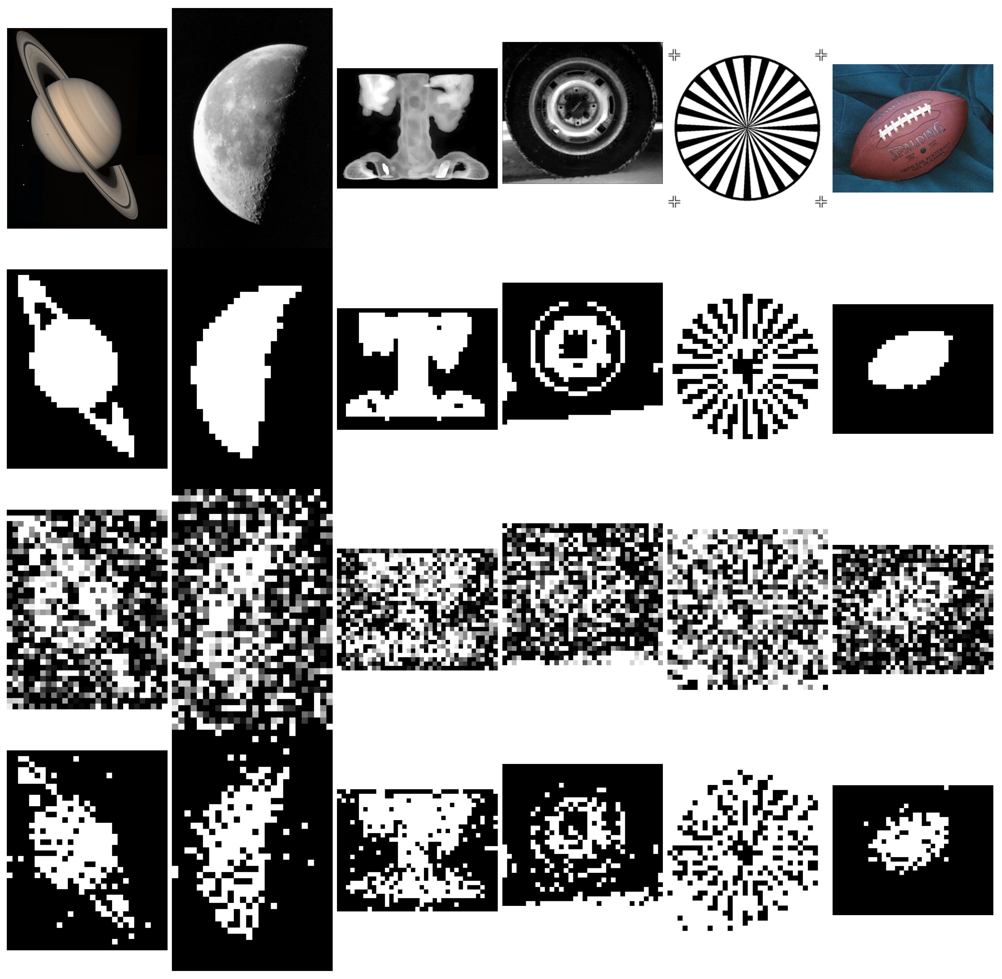
3.3. Application to Binary Image Denoising

The binary image denoising application is formulated as a binary classification problem, where the pixel intensities are either 0 or 1. We used 20 images from Matlab R2022a, as shown in Figure 6, for this task. We followed the same experimental settings as in Section 3.1 and Section 3.2, and conducted two sets of experiments.

In the first set, we downsampled the images by a factor of $\sqrt{1000/\left(AB\right)}$, where A and B are the dimensions of the images, and added Gaussian noise with variance 1 and random seeds 0–9 [48] to the binary images. We split the data into 50% training and 50% test sets, and evaluated the performance of different graph learning schemes using the binary image denoising accuracy defined as:

$$I_{\mathrm{acc}}=\frac{N_{correct}}{N_{test}},$$

(30)

where $N_{correct}$ is the number of correctly predicted pixels and $N_{test}$ is the total number of test pixels. We constructed the graphs using the pixel intensities as the three per-pixel features and Equations (1) and (2), and used the same graph-based classifier [16] as in Section 3.1 and Section 3.2.

In the second set, we focused on the runtime comparison of different graph learning schemes. We normalized the data using the same scheme as in [49].

Figure 7 illustrates some examples of binary image denoising results on six images. The images are, from top to bottom, the original image, binary image, noise-corrupted image, and denoised image.

Table 6. Binary image denoising accuracy $I_{acc}$ (%). Best results are in bold. Chol. = Cholesky. ‘baseline’ denotes the result without using any graph learning methods.

Dataset	Baseline	Chol.	PDcone	HBNB	SGML	PGML	MSGL	MSGL+
cameraman	81.70	83.61	83.73	83.14	82.56	82.54	84.00	83.91
saturn	80.08	82.28	82.28	81.42	81.36	81.51	83.26	83.24
moon	80.85	82.78	82.96	82.11	82.29	82.17	83.27	83.29
spine	73.36	71.74	72.63	73.22	70.97	72.92	74.79	74.77
tire	74.71	77.51	76.92	75.00	77.22	75.47	79.75	79.96
rice	76.56	76.46	76.52	76.56	76.52	76.56	77.03	77.07
testpat1	72.59	76.90	75.56	73.22	74.41	73.26	77.91	77.80
canoe	83.04	83.31	83.04	83.04	83.02	83.04	88.85	88.93
AT3_1m4_02	88.34	89.02	88.86	89.00	88.49	88.40	89.15	89.17
fabric	76.43	76.37	76.62	76.56	75.83	76.64	76.83	76.87
gantrycrane	69.21	69.72	69.61	68.99	68.60	69.15	70.85	70.79
eight	77.25	77.40	77.25	77.25	77.23	77.25	78.34	78.45
circuit	75.45	75.00	75.74	75.59	74.79	75.51	76.23	76.21
mri	79.82	80.55	80.68	80.63	80.35	80.55	80.68	80.68
paper1	73.03	72.87	73.07	73.28	70.92	73.65	74.12	74.10
football	82.79	85.11	84.05	82.89	82.89	83.10	90.19	90.21
glass	74.54	74.71	74.81	74.90	74.71	74.52	75.73	75.77
pears	70.97	71.66	71.48	70.91	70.99	70.83	73.04	72.88
concordaerial	79.94	80.04	80.16	80.22	80.14	79.88	80.24	80.22
autumn	87.62	88.46	87.78	87.68	85.69	88.46	87.80	87.80
best count	0	1	1	0	0	1	10	10
average	77.91	78.78	78.69	78.28	77.95	78.27	80.10	80.11

and Figure 8 present the binary image denoising accuracy and runtime (in log scale) for all 20 images, respectively. The horizontal axis of Figure 8 denotes the 20 images in Figure 6. Each point in the plots represents the average of 10 runs.

Regarding the binary image denoising performance, our proposed MSGL+ achieved the highest accuracy of 80.11% among all the methods. Cholesky, PDcone, HBNB, SGML, PGML, and MSGL obtained 78.78%, 78.69%, 78.28%, 77.95%, 78.27%, and 80.10%, respectively, which are all better than the baseline 77.91%. Similar to Section 3.1, PGML performed worse than the other schemes on average, due to the limited positive graph search space. SGML sometimes performed worse than direct binary image denoising, e.g., for fabric image, due to the constrained, balanced signed graph search space. Also, similar to Section 3.1, Cholesky sometimes converged to a bad local minimum, and thus performed worse than direct classification, e.g., for circuit image. This again demonstrates the superiority of our fast and reliable linear constraint optimization-based graph learning method MSGL+ with the polynomial coefficients $\mathit{\beta }$ as the only optimization variables and extracting the data similarity without learning the pairwise distance metric $\mathbf{M}$ directly.

Our proposed MSGL+ achieved a competitive runtime performance for binary image denoising compared to MSGL, and significantly surpassed the other methods in all experiments. This is because both PGML and SGML have a limited search space (as explained in Section 3.1 for the positive and balanced signed graph, respectively) and linear constraints, as well as the number of features, and they do not require projection operations during the iteration process. The speed gains of MSGL+ over PDcone, Cholesky, HBNB, SGML, PGML, and MSGL were 40.09×, 34.03×, 4.41×, 4.01×, 1.22×, and 0.18×, respectively.

3.4. Application to Time-Series Analysis

We used three publicly available time-series datasets for experiments, CanadaVehicle https://www.goodcarbadcar.net/2021-canada-automotive-sales/ (accessed on 17 December), CanadaVote https://www.ourcommons.ca/members/en/votes (accessed on 17 December), and USVote https://www.congress.gov/roll-call-votes (accessed on 17 December), as described in

Table 7. Time-series datasets named CanadaVehicle, CanadaVote, and USVote. For CanadaVehicle, N denotes the number of car models and J denotes the number of months with car model monthly sales. For CanadaVote, N denotes the number of constituencies and J denotes the number of elections. For USVote, N denotes the number of senators and J denotes the number of elections.

Time-Series Dataset	$(\mathit{N},\mathit{J})$
CanadaVehicle	(218, 24)
CanadaVote	(340, 3154)
USVote	(100, 1320)

. These datasets contain monthly car sales in Canada, parliamentary votes in Canada, and congressional votes in the US, respectively. We first estimated the empirical covariance matrix $\mathbf{C}$ from the data samples in each dataset, and then constructed the graph Laplacian $\mathbf{L}$ by applying graphical Lasso [15] to obtain the sparse inverse covariance matrix $\mathbf{P}$ as follows:

$$\underset{\mathbf{P}\succ 0}{min}\mathrm{Tr}\left(\mathbf{P}\mathbf{C}\right)-logdet\mathbf{P}+{\zeta \left|\right|\mathbf{P}\left|\right|}_1,$$

(31)

where $\zeta >0$ is a regularization parameter that controls the sparsity of $\mathbf{P}$. We set $\mathbf{L}=\mathbf{P}$ for all the subsequent time-series analysis tasks. Note that $\mathbf{L}$ here is not derived from Equation (2), so we did not compare our method with Cholesky, PDcone, HBNB, SGML, or PGML, which require a pairwise distance metric $\mathbf{M}$ to compute $\mathbf{L}$ in Equation (2). We then formulated the time-series analysis task as a binary classification problem, similar to Section 3.1, where the samples, observations, and classes are defined as follows for each dataset. (1) For CanadaVehicle, the samples are the number of car models, the observations are the number of months with car model monthly sales, and the classes are whether the total car sales are above or below 50,000. (2) For CanadaVote, the samples are the number of constituencies, the observations are the number of elections, and the classes are the conservative and liberal parties. (3) For USVote, the samples are the number of senators, the observations are the number of elections, and the classes are the republican and democratic parties. We evaluated the performance of three graph learning schemes: graphical Lasso alone, graphical Lasso combined with MSGL [31], and graphical Lasso combined with our proposed MSGL+ method, which learns $\mathit{\beta }$ given the graphical Lasso-learned $\mathbf{L}$. We generated 10 random splits of 10% training and 90% test data with seeds 0–9 [48] for each dataset, and measured the average binary classification accuracy and runtime of each scheme. We used the same graph-based classifier [16] as in Section 3.1–Section 3.3. We also normalized the data using the same scheme [49] as in Section 3.1 and Section 3.2.

Table 8. Time-series binary classification accuracy (%) with graphical Lasso [15] and our proposed MSGL+ graph learning method on CanadaVehicle, CanadaVote, and USVote.

Method	Lasso	Lasso + MSGL	Lasso + MSGL+
CanadaVehicle	55.74	60.12	80.43
CanadaVote	94.90	95.33	95.33
USVote	85.54	88.84	92.44
number of best	0	1	3
average	78.73	81.43	89.4

shows the results of the time-series binary classification task for the three datasets. It can be seen that our proposed MSGL+ method outperforms the other two schemes, including the Lasso alone and Lasso+MSGL, which demonstrates that our method can effectively exploit the piecewise smoothness property of the graph Laplacian learned from the inverse covariance matrix, without relying on any pairwise distance metric-based data similarity. Again, the box constraint in Equation (29) may lead to sub-optimal performance, as discussed in Section 2.3 and shown in Table 3 and Table 8. As discussed in Section 2.3 and illustrated in Table 8, the box constraint in Equation (29) for MSGL [31] is not necessary and may lead to sub-optimal results.

3.5. Statistical Significance of the Experiments in Terms of the Model Accuracy

Since the classifiers are trained and tested on the same dataset in our experiments, we conducted the mid-p-value McNemar test [50,51] that statistically assesses the accuracies of two classification models. The mid-p-value McNemar test first compares their predicted labels against the true labels, and then it detects whether the difference between the misclassification rates is statistically significant. The null hypothesis of the mid-p-value McNemar test is that Classification Model A and Classification Model B have equal classification accuracy. The alternative hypothesis is that Classification Model A is less accurate than Classification Model B in terms of the classification accuracy. The mid-p-value McNemar test decision $h=1$ indicates to reject the null hypothesis at a certain significance level, and $h=0$ indicates to not reject the null hypothesis at the same significance level. In our experiments, we set three different significance levels, i.e., 5%, 25%, and 50%, respectively.

In our experiments, we set Classification Model A as one of the competing methods (i.e., baseline, Chol., PDcone, HBNB, SGML, PGML, MSGL, Lasso, and Lasso+MSGL) and we set Classification Model B as our proposed MSGL+. For the N runs of each competing method, we obtained the total number of our proposed MSGL+ classification model being more accurate than the competing classification model, divided it by N, and multiplied by 100%, which gave us the percentage of our proposed MSGL+ classification model being more accurate than the competing classification model. Specifically, for baseline, Chol., PDcone, and MSGL, we ran binary classification tests on fifteen datasets (see Section 3.1), multi-classification tests on six datasets (see Section 3.2), and binary image denoising tests on 20 images (see Section 3.3), each of which with 10 runs, which results in $N=410$ runs for each of the aforementioned four competing methods. For HBNB, SGML, and PGML, we ran binary classification tests on 15 datasets (see Section 3.1), and binary image denoising tests on 20 images (see Section 3.3), each of which with 10 runs, which results in $N=350$ runs for each of the aforementioned three competing methods. For Lasso and Lasso + MSGL, we ran time-series analysis tests on three datasets (see Section 3.4), each of which with 10 runs, which results in $N=30$ runs for each of the aforementioned two competing methods.

As shown in

Table 9. McNemar test between competing methods and MSGL+. SL = significance level.

Experiment Type	Binary (Section 3.1)/Multi-Class Classification (Section 3.2), and Binary Image Denoising (Section 3.3)							Time-Series Classification (Section 3.4)
method	baseline	Chol.	PDcone	HBNB	SGML	PGML	MSGL	Lasso	Lasso +MSGL
5% SL	36.34%	16.59%	16.83%	28.86%	33.71%	31.43%	4.88%	53.33%	40.00%
25% SL	61.22%	38.78%	41.95%	52.86%	57.71%	52.86%	15.37%	56.67%	40.00%
50% SL	77.56%	54.63%	60.24%	69.14%	74.29%	69.14%	32.44%	56.67%	40.00%

, the mid-p-value McNemar test detects that 4.88% of the difference between the misclassification rates of our proposed MSGL+ and our previous work MSGL is statistically significant at the 5% significance level. Specifically, 4.88% of the classification experiments of our proposed MSGL+ are statistically more accurate than that of our previous work MSGL at the 5% significance level, 15.37% at the 25% significance level, and 32.44% at the 50% significance level.

4. Discussion

We discuss our main findings based on the experimental results in the previous section in terms of accuracy, runtime, and potential utility in the field of medicine as follows.

4.1. Accuracy

As discussed in Section 3, existing graph learning methods restrict the search space within specific types of graphs, e.g., PGML has a positive graph search space, where the weights within the graph that corresponds to the feature graph are positive only, i.e., the off-diagonal entries within the metric matrix $\mathbf{M}$ are negative only, and thus, it is a significantly smaller search space compared to Cholesky and PDcone; Cholesky and PDcone have a positive graph search space, where the weights within the graph that corresponds to the feature graph can be both positive and negative, i.e., the off-diagonal entries within the metric matrix $\mathbf{M}$ can be negative and positive. SGML has a balanced signed graph search space. Although SGML allows both positive and negative edge weights within the graph that corresponds to the feature graph, the linear constraints of SGML make SGML consist of a non-convex balanced signed graph search space defined by a series of convex search spaces, which may converge to a local minimum and results in sub-optimal performance compared to PDcone. Similar to SGML, HBNB also has a signed graph search space that is not necessarily balanced, but the HBNB requires the projection onto a norm ball that is defined by the first eigenvalue of the metric matrix $\mathbf{M}$, which results in an even smaller search space compared to SGML and much smaller search space compared to Cholesky and PDcone. Graphical Lasso restricts the search space within a positive definite cone with an additional sparsity regularization, which is apparently smaller than that of Cholesky and PDcone. Unlike Cholesky, PDcone, HBNB, SGML, PGML, and graphical Lasso, our proposed MSGL+ graph learning method is not limited by the signs of the off-diagonal entries within the metric matrix $\mathbf{M}$, but defined by the linear combination of the 1-to-P-hop neighborhood graphs parameterized by $\mathit{\beta }$, where the corresponding graph Laplacians can be easily constrained within a positive definite cone using a set of linear constraints without sacrificing the search space. This way, the search space of our formulation is still large enough compared to HBNB, SGML, and PGML, resulting in comparable performance in terms of binary classification accuracy and multi-class classification accuracy, and competitive performance in terms of binary image denoising accuracy and time-series analysis accuracy, shown in Section 3.1, Section 3.2, Section 3.3, and Section 3.4, respectively, while we significantly reduce the computational cost via the linearization of the cone constraint compared to Cholesky and PDcone.

4.2. Runtime

The graph learning methods Cholesky, PDcone, HBNB, SGML, and PGML aim to optimize the metric matrix $\mathbf{M}$, which has $M(M+1)/2$ variables, where M is the number of features, as Table 1 shows. This number can be much larger than the number of variables in our proposed MSGL+ graph learning method, which is the degree P of the polynomial kernel. Our MSGL+ method extracts the data similarity by optimizing the polynomial coefficients $\mathit{\beta }\in {\mathbb{R}}^P$, without directly learning the pairwise distance metric $\mathbf{M}$, as Section 3.1 and Section 3.2 demonstrate. However, the graph construction for a large data size is generally time-consuming, which makes our MSGL+ method slower than SGML and PGML in binary image denoising in Section 3.3, where the number of features is only 3 (the pixel intensity and the pixel locations in two dimensions; see Section 3.3) and the number of samples is much larger than the number of features. Nevertheless, for a small data size, our MSGL+ method becomes faster as the per-sample feature size increases. For Cholesky, PDcone, HBNB, SGML, and PGML, the number of optimization variables in $\mathbf{M}$ or $\mathbf{Q}$ increases dramatically with the per-sample feature size. Finally, as we discussed before, our MSGL+ method is faster than our preliminary work, MSGL, due to the smaller number of variables and linear constraints.

Based on the above discussion, we identify several directions for future research: (1) enhancing the scalability of the model to handle large-scale data, i.e., exploring how to aggregate the information of node batches into a smaller graph that can be efficiently processed by our proposed MSGL+ graph learning pipeline, especially when new samples are added to the existing graph, which is a common scenario in practice; (2) integrating the proposed method with the optimization of the $\mathbf{M}$-defined feature distance and the $A_{ij}$-defined sparsity structure of the graph; (3) selecting the optimal P for different applications; (4) further reducing the number of linear constraints of the objective; (5) applying the proposed method to a broader range of tasks beyond classification, such as regression, clustering, and other low-level image processing tasks besides binary image denoising; and (6) incorporating our proposed MSGL+ into graph neural networks. The interpretability of the neural networks with various loss functions is still an active research topic; the neural networks do not have explicit mathematical objective functions that can be rigorously formulated. Therefore, the comparison between MSGL+ and the neural network-based methods is beyond the scope of this paper.

4.3. Potential Utility in the Field of Medicine

As shown in Table 3 and Table 5, our proposed MSGL+ method outperforms the competing schemes in the biomedical datasets, including Diabetes with eight features, Liver-disorders with five features, and new-thyroid with five features. This indicates that our proposed MSGL+ method has potential to be applied in the field of medicine-related classification.

5. Conclusions

We presented a novel graph learning method, MSGL+, that leverages the power of GSP and model selection to learn a polynomial function $\mathcal{L}={\sum }_{i=1}^P{\beta }_i{\mathbf{L}}^i\succ 0$ that defines a graph Laplacian $\mathcal{L}$. Our method solves a convex optimization problem with a graph Laplacian regularizer and a log determinant term, and uses the Frank–Wolfe method to efficiently update the coefficients $\mathit{\beta }$ under linear constraints. Our method only needs to perform eigen decomposition of a given graph Laplacian $\mathbf{L}$ once, which reduces the computational cost. We demonstrated the superior performance of MSGL+ over existing graph learning methods in various tasks, such as binary and multi-class classification, binary image denoising, and time-series analysis. We also showed that MSGL+ can handle both positive and signed graphs, which are derived from metric matrices or graphical Lasso, respectively. This extension from MSGL greatly expands the applicability of MSGL+, as it can work with any symmetric, positive (semi-)definite matrices that correspond to a (un)signed graph. We suggest that constructing a graph with appropriate feature distance and sparsity prior to applying MSGL+ can further improve the results in practice.

References

1. Rasmussen, C.E.; Williams, C.K.I. Gaussian Processes for Machine Learning (Adaptive Computation and Machine Learning); The MIT Press: Cambridge, MA, USA, 2005. [Google Scholar]
2. Ortega, A.; Frossard, P.; Kovacevic, J.; Moura, J.M.F.; Vandergheynst, P. Graph Signal Processing: Overview, Challenges, and Applications. Proc. IEEE 2018, 106, 808–828. [Google Scholar] [CrossRef]
3. Ortega, A. Introduction to Graph Signal Processing; Cambridge University Press: Cambridge, UK, 2022. [Google Scholar]
4. Cheung, G.; Magli, E.; Tanaka, Y.; Ng, M.K. Graph Spectral Image Processing. Proc. IEEE 2018, 106, 907–930. [Google Scholar] [CrossRef]
5. Leus, G.; Marques, A.G.; Moura, J.M.; Ortega, A.; Shuman, D.I. Graph Signal Processing: History, development, impact, and outlook. IEEE Signal Process. Mag. 2023, 40, 49–60. [Google Scholar] [CrossRef]
6. Zhu, X.; Ghahramani, Z.; Lafferty, J. Semi-supervised Learning Using Gaussian Fields and Harmonic Functions. In Proceedings of the International Conference on Machine Learning, Xi’an, China, 5 November 2003; pp. 912–919. [Google Scholar]
7. Zhai, G.; Min, X. Perceptual image quality assessment: A survey. Sci. China Inf. Sci. 2020, 63, 1–52. [Google Scholar] [CrossRef]
8. Schaeffer, S.E. Survey: Graph Clustering. Comput. Sci. Rev. 2007, 1, 27–64. [Google Scholar] [CrossRef]
9. Berger, P.; Hannak, G.; Matz, G. Graph Signal Recovery via Primal-Dual Algorithms for Total Variation Minimization. IEEE J. Sel. Top. Signal Process. 2017, 11, 842–855. [Google Scholar] [CrossRef]
10. Berger, P.; Buchacher, M.; Hannak, G.; Matz, G. Graph Learning Based on Total Variation Minimization. In Proceedings of the 2018 IEEE International Conference on Acoustics, Speech and Signal Processing (ICASSP), Calgary, AB, Canada, 15–20 April 2018; pp. 6309–6313. [Google Scholar] [CrossRef]
11. Dinesh, C.; Cheung, G.; Bajić, I.V. 3D Point Cloud Super-Resolution via Graph Total Variation on Surface Normals. In Proceedings of the 2019 IEEE International Conference on Image Processing (ICIP), Taipei, Taiwan, 22–25 September 2019; pp. 4390–4394. [Google Scholar] [CrossRef]
12. Dabush, L.; Routtenberg, T. Verifying the Smoothness of Graph Signals: A Graph Signal Processing Approach. arXiv 2023, arXiv:2305.19618. [Google Scholar]
13. Belkin, M.; Matveeva, I.; Niyogi, P. Regularization and semisupervised learning on large graphs. In Proceedings of the Learning Theory, COLT, Banff, AB, Canada, 1–4 July 2004; Lecture Notes in Computer Science. Shawe-Taylor, J., Singer, Y., Eds.; Springer: Berlin/Heidelberg, Germany, 2004; Volume 3120, pp. 624–638. [Google Scholar]
14. Dong, X.; Thanou, D.; Rabbat, M.; Frossard, P. Learning Graphs From Data: A Signal Representation Perspective. IEEE Signal Process. Mag. 2019, 36, 44–63. [Google Scholar] [CrossRef]
15. Friedman, J.; Hastie, T.; Tibshirani, R. Sparse Inverse Covariance Estimation with the Graphical Lasso. Proc. Biostat. 2008, 9, 432–441. [Google Scholar] [CrossRef]
16. Yang, C.; Cheung, G.; Stankovic, V. Alternating Binary Classifier and Graph Learning from Partial Labels. In Proceedings of the Asia-Pacific Signal and Information Processing Association Annual Summit and Conference, Honolulu, HI, USA, 12–15 November 2018; pp. 1137–1140. [Google Scholar]
17. Yang, C.; Cheung, G.; Hu, W. Signed Graph Metric Learning via Gershgorin Disc Perfect Alignment. IEEE Trans. Pattern Anal. Mach. Intell. 2022, 44, 7219–7234. [Google Scholar] [CrossRef]
18. Zhi, Y.C.; Ng, Y.C.; Dong, X. Gaussian Processes on Graphs Via Spectral Kernel Learning. IEEE Trans. Signal Inf. Process. Netw. 2023, 9, 304–314. [Google Scholar] [CrossRef]
19. Zhou, X.; Belkin, M. Semi-supervised Learning by Higher Order Regularization. In Proceedings of the International Conference on Artificial Intelligence and Statistics, JMLR Workshop and Conference Proceedings, Lauderdale, FL, USA, 11–13 April 2011; pp. 892–900. [Google Scholar]
20. Yang, C.; Hu, M.; Zhai, G.; Zhang, X.P. Graph-Based Denoising for Respiration and Heart Rate Estimation During Sleep in Thermal Video. IEEE Internet Things J. 2022, 9, 15697–15713. [Google Scholar] [CrossRef]
21. Gong, X.; Li, X.; Ma, L.; Tong, W.; Shi, F.; Hu, M.; Zhang, X.P.; Yu, G.; Yang, C. Preterm infant general movements assessment via representation learning. Displays 2022, 75, 102308. [Google Scholar] [CrossRef]
22. Tong, W.; Yang, C.; Li, X.; Shi, F.; Zhai, G. Cost-Effective Video-Based Poor Repertoire Detection for Preterm Infant General Movement Analysis. In Proceedings of the 2022 5th International Conference on Image and Graphics Processing (ICIGP ’22), Beijing, China, 7–9 January 2022; Association for Computing Machinery: New York, NY, USA, 2022; pp. 51–58. [Google Scholar] [CrossRef]
23. Li, X.; Yang, C.; Tong, W.; Shi, F.; Zhai, G. Fast Graph-Based Binary Classifier Learning via Further Relaxation of Semi-Definite Relaxation. In Proceedings of the 2022 5th International Conference on Image and Graphics Processing (ICIGP ’22), Beijing, China, 7–9 January 2022; Association for Computing Machinery: New York, NY, USA, 2022; pp. 89–95. [Google Scholar] [CrossRef]
24. Yang, C.; Cheung, G.; Zhai, G. Projection-free Graph-based Classifier Learning using Gershgorin Disc Perfect Alignment. arXiv 2021, arXiv:2106.01642. [Google Scholar]
25. Yang, C.; Cheung, G.; Tan, W.t.; Zhai, G. Unfolding Projection-free SDP Relaxation of Binary Graph Classifier via GDPA Linearization. arXiv 2021, arXiv:2109.04697. [Google Scholar]
26. Fang, X.; Xu, Y.; Li, X.; Lai, Z.; Wong, W.K. Learning a Nonnegative Sparse Graph for Linear Regression. IEEE Trans. Image Process. 2015, 24, 2760–2771. [Google Scholar] [CrossRef] [PubMed]
27. Dornaika, F.; El Traboulsi, Y. Joint sparse graph and flexible embedding for graph-based semi-supervised learning. Neural Netw. 2019, 114, 91–95. [Google Scholar] [CrossRef]
28. Han, X.; Liu, P.; Wang, L.; Li, D. Unsupervised feature selection via graph matrix learning and the low-dimensional space learning for classification. Eng. Appl. Artif. Intell. 2020, 87, 103283. [Google Scholar] [CrossRef]
29. Xing, E.P.; Jordan, M.I.; Russell, S.J.; Ng, A.Y. Distance Metric Learning with Application to Clustering with Side-Information. In Proceedings of the Annual Conference on Neural Information Processing Systems, Vancouver, BC, Canada, 9–11 December 2003; pp. 521–528. [Google Scholar]
30. Wu, X.; Zhao, L.; Akoglu, L. A Quest for Structure: Jointly Learning the Graph Structure and Semi-Supervised Classification. In Proceedings of the ACM International Conference on Information and Knowledge Management, Torino, Italy, 22–26 October 2018. [Google Scholar]
31. Yang, C.; Wang, F.; Ye, M.; Zhai, G.; Zhang, X.P.; Stankovic, V.; Stankovic, L. Model Selection-inspired Coefficients Optimization for Polynomial-Kernel Graph Learning. In Proceedings of the 2021 Asia-Pacific Signal and Information Processing Association Annual Summit and Conference (APSIPA ASC), Tokyo, Japan, 14–17 December 2021; pp. 344–350. [Google Scholar]
32. Egilmez, H.; Pavez, E.; Ortega, A. Graph Learning From Data Under Laplacian and Structural Constraints. Proc. IEEE J. Sel. Top. Signal Process. 2017, 11, 825–841. [Google Scholar] [CrossRef]
33. Jaggi, M. Revisiting Frank-Wolfe: Projection-Free Sparse Convex Optimization. In Proceedings of the International Conference on Machine Learning, Atlanta, GA, USA, 16–21 June 2013; pp. 427–435. [Google Scholar]
34. Mahalanobis, P.C. On the generalized distance in statistics. Proc. Natl. Inst. Sci. India 1936, 2, 49–55. [Google Scholar]
35. Hoffmann, F.; Hosseini, B.; Oberai, A.A.; Stuart, A.M. Spectral analysis of weighted Laplacians arising in data clustering. Appl. Comput. Harmon. Anal. 2022, 56, 189–249. [Google Scholar] [CrossRef]
36. Anis, A.; El Gamal, A.; Avestimehr, A.S.; Ortega, A. A Sampling Theory Perspective of Graph-Based Semi-Supervised Learning. IEEE Trans. Inf. Theory 2019, 65, 2322–2342. [Google Scholar] [CrossRef]
37. Sakiyama, A.; Tanaka, Y.; Tanaka, T.; Ortega, A. Eigendecomposition-Free Sampling Set Selection for Graph Signals. IEEE Trans. Signal Process. 2019, 67, 2679–2692. [Google Scholar] [CrossRef]
38. Shuman, D.I.; Narang, S.K.; Frossard, P.; Ortega, A.; Vandergheynst, P. The Emerging Field of Signal Processing on Graphs: Extending High-dimensional Data Analysis to Networks and Other Irregular Domains. Proc. IEEE Signal Process. Mag. 2013, 30, 83–98. [Google Scholar] [CrossRef]
39. Romero, D.; Ma, M.; Giannakis, G.B. Kernel-Based Reconstruction of Graph Signals. IEEE Trans. Signal Process. 2017, 65, 764–778. [Google Scholar] [CrossRef]
40. Smola, A.J.; Kondor, R. Kernels and Regularization on Graphs. In Proceedings of the Learning Theory and Kernel Machines, Washington, DC, USA, 24–27August 2003; Schölkopf, B., Warmuth, M.K., Eds.; Springer: Berlin/Heidelberg, Germany, 2003; pp. 144–158. [Google Scholar]
41. Boyd, S.; Vandenberghe, L. Convex Optimization; Cambridge University Press: Cambridge, UK, 2009. [Google Scholar]
42. Papadimitriou, C.; Steiglitz, K. Combinatorial Optimization; Dover Publications, Inc.: Mineola, NY, USA, 1998. [Google Scholar]
43. Raphson, J. Analysis Aequationum Universalis; University of St Andrews: St Andrews, UK, 1690. [Google Scholar]
44. Hu, W.; Gao, X.; Cheung, G.; Guo, Z. Feature graph learning for 3D point cloud denoising. IEEE Trans. Signal Process. 2020, 68, 2841–2856. [Google Scholar] [CrossRef]
45. Yang, C.; Cheung, G.; Hu, W. Graph Metric Learning via Gershgorin Disc Alignment. In Proceedings of the IEEE International Conference on Acoustics, Speech and Signal Processing, Barcelona, Spain, 4–8 May 2020. [Google Scholar]
46. Golub, G.H.; Van Loan, C.F. Matrix Computations, 3rd ed.; The Johns Hopkins University Press: Baltimore, MD, USA, 1996. [Google Scholar]
47. Weinberger, K.Q.; Saul, L.K. Distance metric learning for large margin nearest neighbor classification. J. Mach. Learn. Res. 2009, 10, 207–244. [Google Scholar]
48. Russell, S.; Norvig, P. Artificial Intelligence: A Modern Approach, 3rd ed.; Prentice Hall Press: Hoboken, NJ, USA, 2009. [Google Scholar]
49. Dong, M.; Wang, Y.; Yang, X.; Xue, J. Learning Local Metrics and Influential Regions for Classification. IEEE Trans. Pattern Anal. Mach. Intell. 2020, 42, 1522–1529. [Google Scholar] [CrossRef]
50. Mcnemar, Q. Note on the sampling error of the difference between correlated proportions or percentages. Psychometrika 1947, 12, 153–157. [Google Scholar] [CrossRef]
51. Fagerland, M.W.; Lydersen, S.; Laake, P. The McNemar test for binary matched-pairs data: Mid-p and asymptotic are better than exact conditional. BMC Med. Res. Methodol. 2013, 13, 91. [Google Scholar] [CrossRef]
Figure 1. Illustration of the graph learning, graph classifiers, and graph signal priors in the context of graph-based classification.
Electronics 13 00044 g001
Figure 2. Illustration of the convex search space (in light orange) for β 1 and β 2 when P = 3 .
Electronics 13 00044 g002
Figure 3. Runtime (ms) on binary classification. The horizontal axis of each plot denotes the datasets in ascending order of the runtime of the problem size. Each point denotes the average of 10 runs.
Electronics 13 00044 g003
Figure 4. Runtime for binary datasets Madelon (left) and Colon−cancer (right) with various data and feature sizes, respectively.
Electronics 13 00044 g004
Figure 5. Runtime on multi-class classification. The horizontal axis of each plot denotes the datasets in ascending order of the runtime of the problem size. Each point in the plots denotes the average of 10 runs.
Electronics 13 00044 g005
Figure 6. Matlab images used for denoising. From left to right and top to bottom: cameraman, saturn, moon, spine, tire, rice, testpat1, canoe, AT3_1m4_02, fabric, gantrycrane, eight, circuit, mri, paper1, football, glass, pears, concordaerial, and autumn.
Electronics 13 00044 g006
Figure 7. Sample binary image denoising results on saturn, moon, spine, tire, testpat1, and football. From top to bottom: original, binary, noise-corrupted, and denoised image.
Electronics 13 00044 g007
Figure 8. Runtime on binary image denoising.
Electronics 13 00044 g008