A Voltage-Level Optimization Method for DC Remote Power Supply of 5G Base Station Based on Converter Behavior

Abstract

Unlike the concentrated load in urban area base stations, the strong dispersion of loads in suburban or highway base stations poses significant challenges to traditional power supply methods in terms of efficiency and cost. High-voltage direct current (HVDC) remote supply have better application potential in this scenario due to their low transmission losses, attracting much attention. However, existing research has problems such as ambiguous optimal power supply distance under different voltage levels and a lack of behavioral models for converters. Therefore, this paper starts from the behavior of underlying converters, analyzes the loss composition of different converters in HVDC long-distance supply, and establishes a refined model for converters by determining the mathematical relationship between converter losses and operating power. Considering the economic feasibility of power supply solutions throughout the lifecycle, a modeling method is proposed that optimizes the voltage level of converters considering the behavior of converters for different supply distances. The optimal voltage level for different supply distances is discussed, and the effectiveness of the model is verified through examples, providing valuable guidance for optimizing the voltage level in HVDC long-distance supply for 5G base stations.

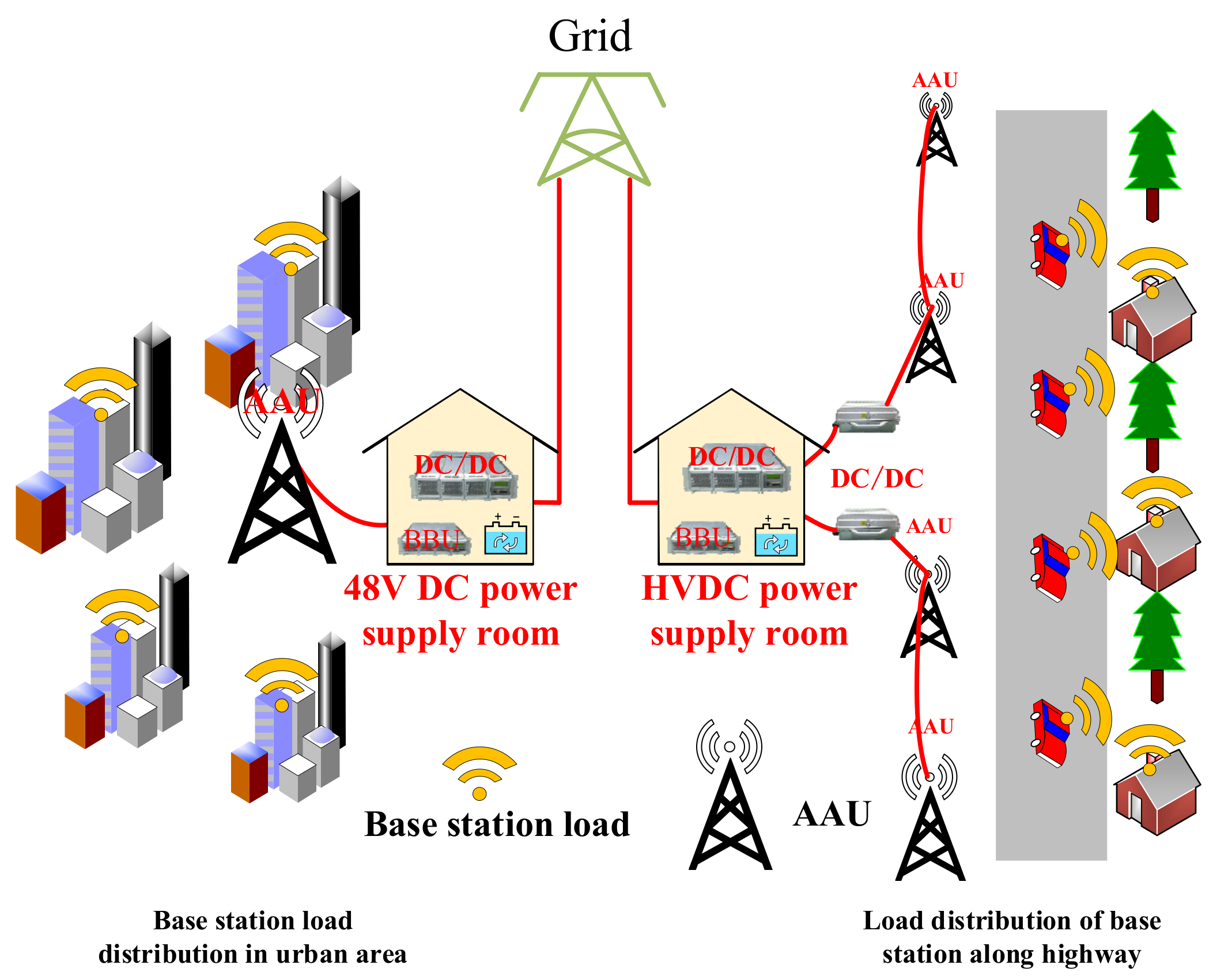
1. Introduction

The all-area laying of 5G base stations is an important foundation for realizing the 5G communication strategy [1,2]. How to lay 5G base stations in all areas according to the load distribution characteristics of base stations in differentiated scenarios is a key step to realizing the 5G communication strategy. Figure 1 shows the basic distribution structure of base station load under two typical scenarios. Figure 1 shows the load distribution of the base station in the urban area on the left, which is characterized by relatively concentrated load and high density [3,4]. The installation and power supply of the active antenna unit (AAU) and base band unit (BBU) of the main equipment of the 5G base station are usually arranged nearby [5]. Figure 1 (the right) shows the distribution of base stations in the suburbs or along the highway [6,7,8,9]. Different from the load distribution of base stations in urban areas, the load of suburban or highway is highly dispersed, which often requires a long-distance power supply for communication equipment [10,11]. As shown in Figure 2, power factor correction (PFC) and battery management (BMS) are used to improve power factor and battery utilization, respectively. The common base station power supply system is powered by a 48 V DC bus, which is connected to the DC load and backup battery [12,13]. With the increase in power supply distance, 48 V low-voltage DC power supply will not only increase the cost but also cause problems such as excessive line voltage drop, which cannot meet the basic power supply requirements of communication equipment, and have adverse effects on efficiency and economy [14,15].

The high-voltage DC remote power supply scheme, as shown in Figure 3, can effectively reduce the line power supply current by improving the power supply level of the office voltage. On the one hand, the demand for transmission cables is reduced; on the other hand, the line loss and voltage drop are reduced. Compared with high voltage alternating current (HVAC) power supply, HVDC transmission has higher transmission efficiency and longer power supply distance [16]. Therefore, this scheme has attracted more attention in recent years and has become an important choice for remote power supply of base stations [17,18,19]. The existing research mainly focuses on the basic structure, application, and scheme design of HVDC remote power supply and the comparison with other power supply schemes [20,21,22,23,24,25,26,27,28,29]. For example, the authors of [20,21] introduced the strong dispersion characteristics of some loads of 5G base stations but did not discuss the new power supply type according to the distribution characteristics of the load. Based on the above, the authors of [22,23] proposed the HVDC remote power supply type suitable for strongly distributed loads, and the authors of [23] also made a more comprehensive comparison with other power supply types. The authors of [24,25,26,27] outlined how to plan, design, and deploy HVDC remote power supply schemes, but in the design process, there is a lack of discussion and analysis of converter types and no clear definition of voltage level and power supply distance. The authors of [28,29] emphasized the voltage level and effective power supply distance of this structure but did not consider the influence of the converter behavior in the power supply structure. However, in the above research, the output voltage level range of the near terminal converter is often set wide usually between 240 and 700 V, and the matching scheme between the power supply distance and voltage level is not given. In addition, the above-mentioned literature rarely considers the converter behavior in the power supply system when optimizing various schemes; it tends to neglect the dynamic variation process of converter efficiency under different operating conditions, treating converter efficiency in practical engineering operations as a constant value. Consequently, this leads to deviations in the final optimization outcomes.

Therefore, this paper starts with the underlying converters of the DC remote power supply system. By analyzing the loss components of the near terminal and remote terminal converters, it establishes the functional relationship between converter efficiency and operating power. Based on this, the optimization results with the converter behavior considered in this paper are compared with those without considering the converter behavior, highlighting the influence of the converter behavior on the optimization results in actual operation and the optimal matching scheme of the power supply distance and voltage level in the DC power supply scheme is obtained.

2. Model Building

According to the power supply structure shown in Figure 3, the optimization of voltage level with the near terminal converter is studied. The system composition is shown in Figure 4. Due to the wide variety of converters with a high step-up ratio, this paper selects the most basic Boost and cascade Boost converters for analysis. The main reason is that these two converters have the basic characteristics of a wide step-up range, flexible design, and stable output voltage and have received extensive attention in the industry [30]. At the same time, considering that in the actual working process, the step-up ratio of the boost converter is limited by the parasitic parameters of the circuit and components [31,32,33], the step-up ratio here is set at 1–5 times. Therefore, the near-terminal converter is divided into two cases. When the output voltage of the near terminal is less than 240 V, a Boost circuit is selected. When the output voltage of the near terminal is greater than or equal to 240 V, two Boost converters are selected to work in cascade. To reduce the voltage, the more mature LLC converter in the communication power supply is selected.

2.1. Converter Loss Analysis

Based on determining the topological type, analyzing the loss distribution of the converter, and determining its calculation method are the main steps to establish the refined efficiency model of the converter. Combined literature [34,35], its main loss expression is as follows:

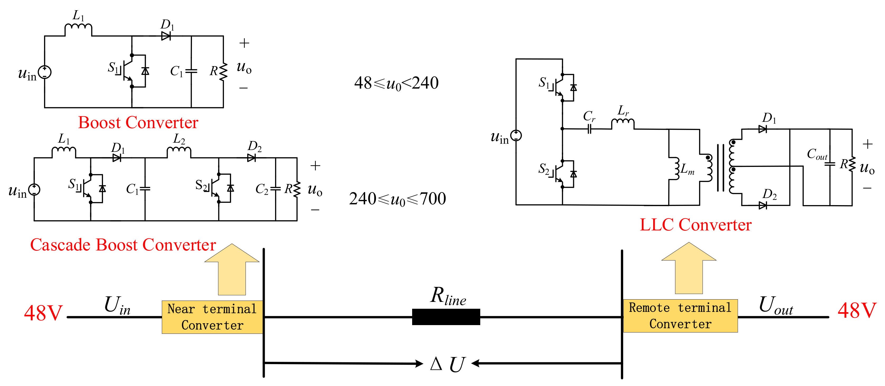
• The switching loss in Boost converter or Cascade Boost converter:

$$\left\{\begin{array}{l}{P}_{loss\_mos}=D\cdot I_{mos}^2\cdot R_{mos}+0.5 fV{I}_{mos}(t_r+t_f)\\ I_{mos}=\frac{P_{load}}{u_{in}}\end{array}\right.$$

(1)

P_{loss_mos} is the total loss in the switch; D is the duty cycle; I_mos is the current flowing through the switch; R_mos is the on-resistance of the switch; f is the switching frequency; V is the turn-off voltage of the switch; t_r and t_f are the opening and closing time of the switch, respectively; P_load indicates the running power; u_in indicates the input voltage.

2.

The diode loss in Boost converter or Cascade Boost converter:

$$\left\{\begin{array}{l}{P}_{loss\_dio}=k_1\cdot I_{Dio\_ave}+k_2\cdot I_{Dio\_rms}^2\\ I_{Dio\_ave}=\frac{P_{load}}{u_{in}}(1-D)\\ I_{Dio\_rms}=\sqrt{{(\frac{P_{load}}{u_{in}})}^2\cdot (1-D)}\end{array}\right.$$

(2)

P_{loss_dio} is diode loss; I_{Dio_ave} is the average current flowing through the diode; I_{Dio_rms} is the effective current flowing through the diode; k₁ and k₂ are loss coefficients, generally determined by the type of diode.

3.

The inductance loss in Boost converter or Cascade Boost converter:

$$\left\{\begin{array}{l}{P}_{core}=V_e{k}_3{f}^{a_1}\Delta B^{a_2}\\ P_{cu}=I_L^2\cdot R_{cu}\\ \Delta B=\frac{L\cdot \Delta i_L}{N\cdot A_e}\\ I_L=\frac{P_{load}}{u_{in}}\end{array}\right.$$

(3)

P_core and P_cu are, respectively, the iron loss and copper loss at the inductance of the converter; V_e is the core volume; k₃, a₁ and a₂ are constants, which are related to the core material; R_cu is winding resistance; ΔB is the changing magnetic induction intensity; A_e is the cross-sectional area of the magnetic core; Δi_L is inductance current ripple, generally a constant value; N is the number of turns wound; I_L is the current flowing through the inductor.

4.

The switching loss composition in LLC is shown in Formula (4):

$$\left\{\begin{array}{l}{P}_{mos\_LLC}=I_{mos\_LLC\_rms}^2\cdot R_{mos}+\frac{I_{off}^2\cdot t_f^2\cdot f_s}{48\cdot C_{zvs}}\\ I_{mos\_rms}=\frac{1}{2}\sqrt{{(\frac{\pi }{2}\cdot \frac{I_0}{n}\cdot \frac{f_r}{f_s})}^2+{[\frac{n\cdot (u_{out}+V_{fd})}{4\cdot L_m\cdot f_s}]}^2}\\ I_{off}=\frac{n\cdot u_{out}}{4\cdot L_m\cdot f_s}\\ I_0=\frac{P_{load}}{u_{out}}\end{array}\right.$$

(4)

P_{mos_LLC} is the switching tube loss in the LLC converter; f_s is the operating frequency; C_zvs is the sum of the equivalent junction capacitance and stray capacitance of the switch; f_r is the first resonant frequency; u_out is the 48 V output voltage of LLC; V_fd is the conduction voltage of diode; n is the transformer turn ratio; L_m is the transformer excitation inductance.

5.

The loss composition of the diode in the LLC converter is shown in Formula (5):

$$\left\{\begin{array}{l}{P}_{dio\_LLC}=V_{fd}\cdot I_{Dio\_ave}+Q_j\cdot u_{out}\cdot f_s\\ I_{Dio\_ave}=\frac{P_{load}}{2\cdot u_{in}}\end{array}\right.$$

(5)

P_{dio_LLC} is the loss in the diode; Q_j is the junction capacitance of the diode. It depends on the type of diode.

The resonant inductor loss and transformer loss in LLC are similar to Formula (3), and the description is not repeated.

2.2. Refined Efficiency Model of the Converter

Referring to the loss analysis of the converter in Section 2.1, it can be seen that the loss in the converter is mainly generated by switching components, magnetic components (inductors, transformers), and capacitors. In the case of constant duty cycle and switching frequency, according to the relationship between the loss and the converter operating power, it can be divided into three categories: (1) constant, such as magnetic core iron loss; (2) primary items, such as switching loss, diode conduction loss; (3) secondary items, such as copper loss in magnetic components, the turn-on loss in switches, and capacitance loss. According to the three types of relations between converter loss and operating power, the mathematical model between converter loss P_lost, and operating power P_load can be expressed as follows:

$$P_{lost}=a_0+b_0{P}_{load}+c_0{P}_{load}^2$$

(6)

The relationship between the real-time efficiency of the converter, the loss P_lost, and the operating power P_load is shown as follows:

$$\eta =1-\frac{P_{lost}}{P_{load}}$$

(7)

Combined with Formulas (6) and (7), the functional relationship between the converter efficiency η and the operating power P_load can be expressed as follows:

$$\eta =1-\frac{a_0}{P_{load}}-b_0-c_0{P}_{load}=\frac{a}{P_{load}}+b+c{P}_{load}$$

(8)

Formula (8) is the refined efficiency model of the converter, in which a₀, b₀, c₀, a, b, and c are all fitting coefficients. Based on determining the converter type, power level, and device type, the efficiency under three different loads can be calculated. Taking the efficiency under 100%, 50%, and 25% loads as an example, the calculation method is shown in Formula (9):

$$\left\{\begin{array}{l}a=\frac{2{\eta }_{25}-3{\eta }_{50}+{\eta }_{100}}{3}\\ b=-2{\eta }_{25}+5{\eta }_{50}+2{\eta }_{100}\\ c=\frac{4{\eta }_{25}-12{\eta }_{50}+8{\eta }_{100}}{3}\end{array}\right.$$

(9)

where η₁₀₀, η₅₀, and η₂₅ are the efficiency of the converter under 100%, 50%, and 25% load, respectively.

2.3. DC Remote Supply System Level Economic Model

Based on the refined efficiency models of converters with different voltage levels, the optimization of voltage levels is studied with the whole life cycle cost (LCC) as the economic evaluation index.

The cost C_LCC of the whole life cycle is shown in Equation (10).

$$C_{LCC}=C_I+C_O$$

(10)

where C_I is the initial investment cost; and C_o is the operating cost.

• Initial investment cost.

The initial investment cost is mainly the purchase cost of related equipment during the construction of the power supply structure of the base station. To calculate the net present value cost during the whole life cycle, the impact of the discount rate should be considered [36]. The initial investment cost calculation is shown in Equation (11).

$$C_I=(C_I^{trans}+C_I^{line})\times \frac{\gamma {(1+\gamma )}^{Lc}}{{(1+\gamma )}^{Lc}-1}\times L_C$$

(11)

where γ is the discount rate; L_C is the system life cycle; $C_I^{trans}$ and $C_I^{line}$ respectively represent the cost of converter and cable. The specific calculation formula is shown in Equation (12).

$$\left\{\begin{array}{l}{C}_I^{line}=Q_{line}\cdot L_{line}\\ C_I^{trans}={\displaystyle \sum _{h=1}^H(Q_{trans\_h}\cdot N_{trans\_h})}\end{array}\right.$$

(12)

where Q_line is the price of cable per unit length; L_line indicates the laying length of the cable; Q_{trans_h} is the unit price of the converter; N_{trans_h} is the number of converters used.

2.

Operating costs

The operating cost is mainly caused by the loss in converters and lines and the maintenance cost during the operation period. The calculation formula is as follows:

$$C_o=C_o^{trans}+C_o^{line}+C_M$$

(13)

where $C_o^{trans}$ is the converter loss cost; $C_o^{line}$ is line loss cost; C_M is the maintenance cost. Converter loss comes from the efficiency of the converter, and maintenance costs mainly come from the maintenance of conventional cable maintenance converter equipment. The specific expression is as follows:

$$\left\{\begin{array}{l}{C}_o^{trans}={\displaystyle \sum _{i=1}^m(\beta \cdot {\eta }_i\cdot P_{t_i}\cdot t_i)}\\ C_o^{line}={\displaystyle \sum _{i=1}^m\beta \cdot {(\frac{P_{t_i}}{U_{Distal}})}^2\cdot R_{line}\cdot t_i}\\ C_M={\displaystyle \sum _{t=1}^{L\mathrm{c}}\frac{a_t{C}_I}{{(1+\gamma )}^t}}\end{array}\right.$$

(14)

where m is the total operating time of the converter; β is the purchase price of electricity; η_i is the converter efficiency in the period; P_ti is the converter power of the period; U_Distal is the input voltage of the remote terminal LLC converter; t_i is the period length, the greater the total power consumption, resulting in higher line loss cost and operating cost; a_t is the maintenance factor of year t, denoting the numerical relationship between maintenance costs and the initial investment. A higher value of at leads to higher maintenance costs, resulting in higher operating cost; L_C represents the full life cycle based on the year.

3. Near Terminal Converter Voltage Level Optimization

3.1. Objective Function

$$\min C_j{}_{LCC}=\min (C_j{}_I+C_j{}_O)$$

(15)

where j is the voltage level; C_jI, C_jO, and C_jLCC are the initial investment cost, operating cost, and life cycle cost under the determined voltage level, respectively.

3.2. Constraints

• Constraints on line power balance

$$P_{Distal\_in}={\eta }_1{P}_{Local\_in}-P_{loss\_line}$$

(16)

η₁ is the efficiency of the current-terminal converter; P_{Local_in} is the input power of the converter at the near terminal; P_{loss_line} indicates the power loss in the line; P_{Distal_in} indicates the input power of the remote terminal LLC converter.

2.

Power balance constraints of 5G base station

To meet the normal operation of the base station, the design of each part of the scheme should meet the following requirements:

$$P_{5G}={\eta }_2{P}_{Distal\_in}$$

(17)

P_5G is the load power of the 5G base station; η₂ is the efficiency of the remote terminal LLC converter.

3.

Constraints on wire diameter selection

$$I_N\ge 1.5I_l$$

(18)

I_N the rated current of the inductor or cable; I_l is the maximum current flowing through a wire or cable.

4.

Window coefficient constraint

$$a_m\le 0.35$$

(19)

m is the magnetic core type; a_m is the window coefficient of the current magnetic core. The window coefficient is less than 0.35 to ensure that the selected magnetic core can be wound to produce the required inductance value.

5.

components selection constraints

The voltage variation in different schemes is too large, so the component selection should meet the stress constraints of the voltage and current of the components.

$$\left\{\begin{array}{l}{V}_{N\_r}\ge 1.5V_{ds\_r}\\ I_{N\_r}\ge 1.5I_{ds\_r}\end{array}\right.$$

(20)

V_{N_r} and I_{N_r} are the rated voltage and rated current of the components. V_{ds_r} and I_{ds_r} are the voltage and current stresses on the components, the magnitude of which is determined by the topology type, and r is the type of components.

6.

Line loss constraints

$$P_{loss\_line}\le 0.1{\eta }_1{P}_{Local\_in}$$

(21)

The line loss power shall not exceed 10% of the output power of the converter at the near terminal.

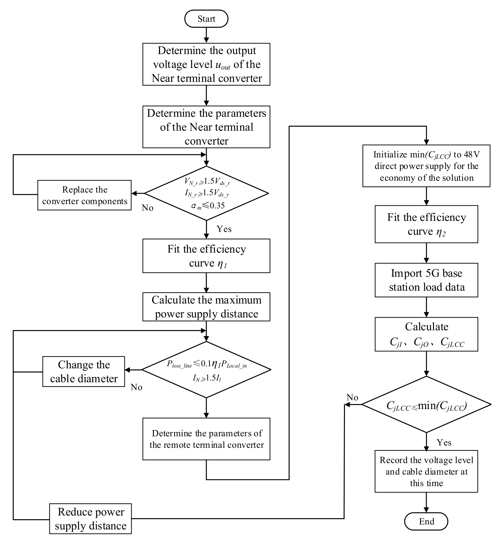
3.3. Flowchart Description

The optimization problem is solved using the traversal algorithm. Its basic solution process is shown in Figure 5. Firstly, determining the output voltage of the near terminal converter to determine the type of the near terminal converter. In order to ensure the normal operation of the converter, all components in the converter must work normally under the current voltage level. Therefore, if constraint conditions (19) and (20) are not met, the converter component type needs to be replaced. Secondly, the efficiency curve η₁ of the near terminal converter is fitted according to Formulas (6)–(10) for the subsequent calculation of converter losses, and the maximum power supply distance is calculated under the current voltage level. Thirdly, we determined whether the cable diameter meets constraint conditions (18) and (21) at this time; if not, the cable diameter needs to be replaced. This step is to ensure that the electrical energy can be normally transmitted to the electrical equipment of the base station. Fourthly, min_(CjLCC) is initialized as the economy of the 48 V direct power supply scheme, and the efficiency curve η₂ of the remote terminal converter is fitted for the subsequent calculation of the loss in the remote terminal converter. Finally, C_jLCC at this time is calculated to determine the size relationship between C_jLCC and min_(CjLCC). If the C_jLCC is smaller, the voltage level and supply distance at this time are recorded, and the optimal matching scheme between voltage level and power supply distance can be obtained.

4. Simulations

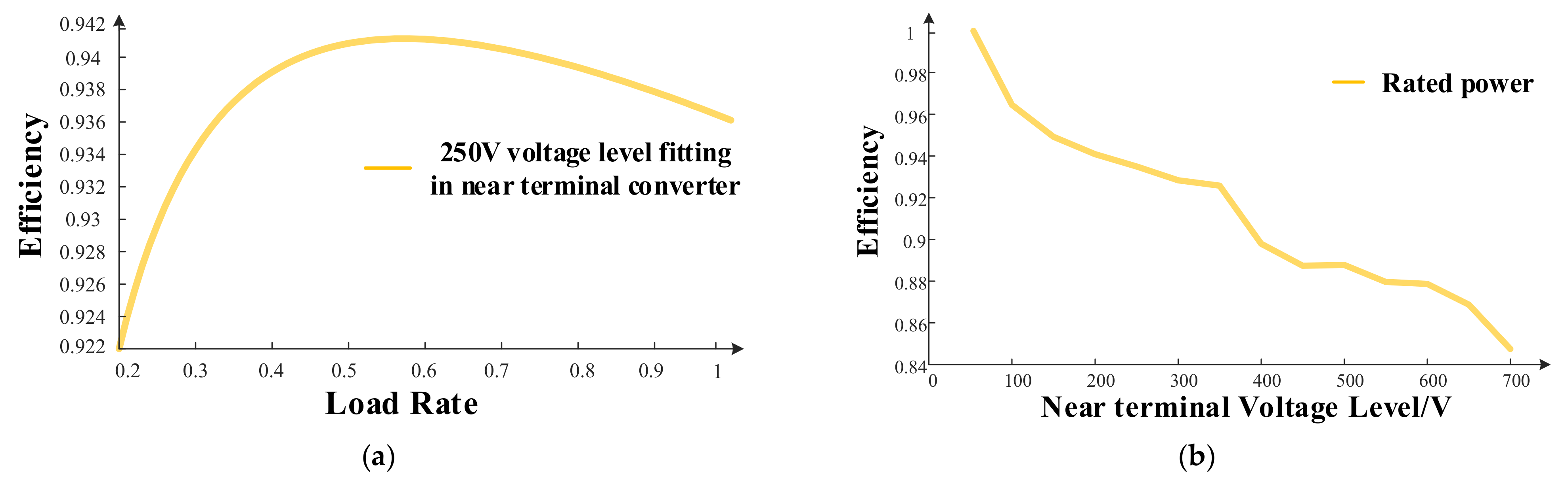
4.1. Converter Efficiency Curve Fitting

In this paper, the 5G load of a highway in Guangxi Province is selected as the basic reference. To ensure the normal operation of the topology, this paper takes 50 V as the step to optimize the voltage level. Among them, 48 V voltage levels are used for direct power supply, and 100–700 V voltage levels are obtained by DC/DC converters. The cables and other parameters are shown in

Table 1. Cable and other parameters.

Parameters	Value
Power purchase price/CNY	0.667
1 mm2 cable/CNY/m	2.52
1.5 mm2 cable/CNY/m	3.26
2.5 mm2 cable/CNY/m	5.06
4 mm2 cable/CNY/m	7.49
6 mm2 cable/CNY/m	10.73
10 mm2 cable/CNY/m	17.06
16 mm2 cable/CNY/m	24.59
25 mm2 cable/CNY/m	38.92
35 mm2 cable/CNY/m	53.87
50 mm2 cable/CNY/m	72.44

, and the CNY represents the Chinese Yuan.

In order to match the power level of the current mainstream AAU equipment, the power of a single near terminal and remote terminal converter is set to 1500 W in this paper. On this basis, aiming at the voltage range of 48–700 V, this paper compares the schemes under 14 voltage levels with a 50 V step length. Based on considering the refined model of the converter, Figure 6a–d shows the fitting results and specific analysis of converter efficiency curves at different voltage levels and all converters operate at rated power.

The efficiency of near-terminal and remote terminal converters at the 250 V voltage level was selected for curve fitting. Figure 6b,d shows the variation trend between the efficiency and voltage levels of the converter at the rated power level. As shown in Figure 6b, the near-terminal converter uses Boost or Cascade Boost as an example. The efficiency of the converter gradually decreases as the voltage level increases. In particular, the increase in voltage level is accompanied by the decrease in the current of the switch, thus reducing the conduction loss. However, the increase in voltage level increases the voltage stress of the switch. The high-stress switch is accompanied by large on-resistance and long turn-on and turn-off time, which increases the switching loss. Therefore, the overall loss in the converter shows an increasing trend, and the overall efficiency shows a downward trend with the increase in voltage level.

The remote terminal LLC converter operates between the first resonant frequency and the second resonant frequency to enable the primary switch to operate in the zero voltage switch (ZVS) state and the secondary switch to operate in the zero current switch (ZCS) state [37]. Referring to Figure 6d, compared with the 48 V direct power supply, when the voltage class gets to 100–700 V, the power supply scheme has converter loss, so the overall efficiency is reduced. With the increase in voltage level, the current flowing through the switch on the primary side of the LLC converter gradually decreases, and the conduction loss decreases. Since the primary switch has no turn-on loss and the secondary diode has no turn-off loss, the overall efficiency curve increases gradually with the increase in voltage level. The voltage level continues to increase, and the turn-off loss in the switch and the turn-off loss in the secondary switch are the main losses, and the overall efficiency decreases slightly.

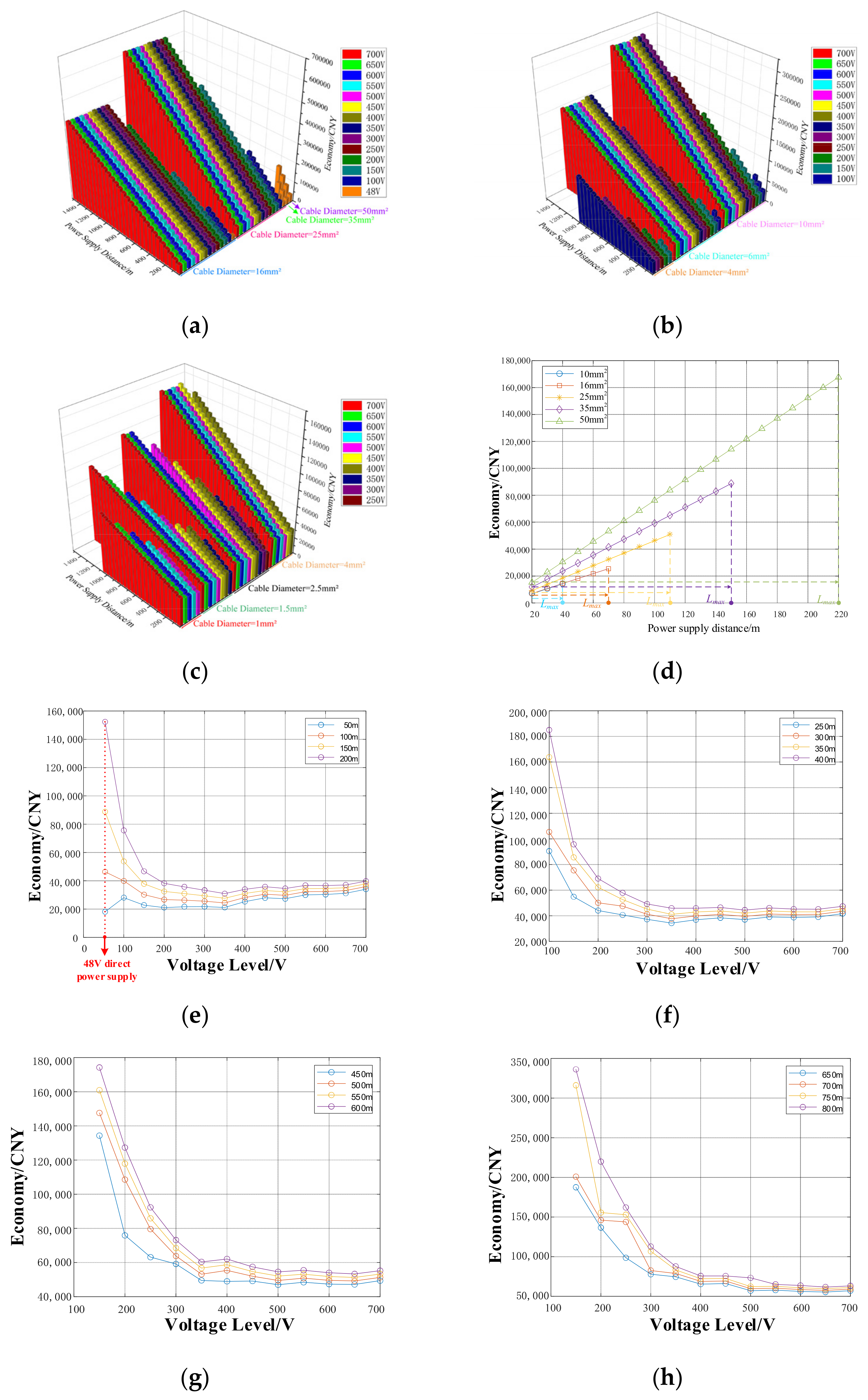
4.2. Analysis of Optimization Results

Figure 7a–c is an economic comparison of power supply schemes under different cable diameters. It can be seen from this figure that with the increase in voltage level, the available types of cables are expanded, and the power supply schemes tend to be diversified. Figure 7d shows the economic comparison of different cable types at different power supply distances under the 48 V direct power supply scenario. To obtain the optimal matching scheme between voltage level and power supply distance, the optimal economic curves corresponding to different voltage levels at the same supply distance are required, and the results are shown in Figure 7e–j.

As shown in Figure 7e, the 48 V direct power supply mode has the optimal economy when the power supply distance is about 50 m during the whole life cycle. However, as the power supply distance increases to more than 100 m, the cost of changing the diameter of the line while meeting the constraint of line loss is gradually higher than the cost of increasing the voltage level. Therefore, the 48 V direct power supply scheme is unnecessary to consider as the power supply distance continues to increase. Similarly, the 100 V solution is also abandoned in Figure 7f,g. With the increase in the power supply distance, the required cable cost gradually rises, and the advantages of high voltage levels gradually appear. According to the installation distance of 5G base stations on different occasions, the station spacing in the central urban area is 240–300 m, the new urban area is 300–350 m, the township is 400–500 m, and other remote areas are 1000–1200 m. Combined with the optimization results from Figure 7e–j, the optimal power supply distance and corresponding cost components under different voltage levels can be obtained, as shown in

Table 2. The optimal economic solution for different voltage levels.

Voltage Level/V	Power Supply Distance/m	Cable Diameter/mm2	Economy/CNY
48	50	10	17,882
350	100	1.5	24,367
350	150	1.5	27,611
350	200	1.5	30,906
350	250	1.5	34,254
350	300	1.5	37,657
350	350	1.5	41,117
500	400	1.5	44,492
500	450	1.5	46,995
650	500	1	49,222
650	550	1	51,279
650	600	1	53,347
650	650	1	55,427
650	700	1	57,518
650	750	1	59,621
650	800	1	61,736
650	850	1	63,863
650	900	1	66,002
650	1100	1.5	76,299
650	1150	1.5	78,495
650	1200	1.5	80,696
700	950	1	69,210
700	1000	1	71,244
700	1050	1	73,288

.

Table 2 shows that when the base station is installed in the central city and the new city, the optimal voltage level is 350 V, and the cable diameter is 1.5 mm². When installed in towns and villages, the optimal voltage level is 500 V when the power supply distance is 400–450 m, and the cable diameter is 1.5 mm². When the power supply distance is 500 m, the optimal voltage level is 650 V, and the cable diameter is 1 mm². When installed in other remote areas, the optimal voltage level is 700 V when the power supply distance is 1000–1100 m, and the cable diameter is 1 mm². When the power supply distance is 1100–1200 m, the optimal voltage level is 650 V, and the cable diameter is 1.5 mm².

4.3. Comparative Analysis

In the traditional power supply scheme, the converter efficiency is usually fixed. This traditional converter model ignores the coupling relationship between the converter efficiency, voltage level, and load rate in the actual operation process, resulting in inaccurate economic calculation results. Therefore, a refined converter model considering the above coupling relationship is proposed in this paper. With the power supply distance of 50–200 m as the application background, it is compared with the traditional converter model with constant efficiency. The results are shown in Figure 8a–d.

When the converter efficiency is 100% (Figure 8b), the total cost of the scheme is mainly composed of line loss cost and cable cost. At the same power supply distance, the higher the voltage level, the smaller the current flowing on the cable, and the lower the demand for the cable, so the total cost of the scheme decreases with the increase in the voltage level. When the converter efficiency is not 100% (Figure 8c,d), the 48 V direct power supply scheme has a lower cost because it has no converter loss when the power supply distance is relatively close. However, with the increase in the power supply distance, the lower the voltage level, the higher the demand for cables, and the cost required for the 48 V direct power supply scheme rises sharply. At this time, the advantages of the HVDC power supply scheme are gradually reflected, but its effect is still that the higher the voltage level, the lower the cost of the scheme. The main reason is that the traditional converter model ignores the loss cost accumulated by the dynamic change in converter efficiency under different voltage levels in actual operation, amplifies the positive benefit of voltage level to line loss, resulting in a large deviation in economic calculation results, and the optimal matching relationship between voltage level and power supply distance is fuzzy.

Therefore, the refined model of the converter proposed in this paper establishes the functional relationship between the converter efficiency and the load rate based on the determined voltage level and obtains the multi-dimensional matching relationship between the voltage level and the power supply distance by taking the economy as the objective function (as shown in Figure 8e). The final optimization results are more close to reality, and the reliability of the optimization results is higher.

5. Conclusions

Aiming at the problems in the current design of the HVDC remote supply scheme for 5G base stations, such as the large voltage step-up range of the converter at the near terminal and the ambiguity of the optimal voltage level at different power supply distances, this paper proposes a voltage level optimization method for DC remote power supply based on converter behavior and draws the following conclusions for different power supply distances:

• The output efficiency of the converter is constantly changing in the actual operation, and if it is assumed to be constant in the design of the scheme, the final optimization result will be seriously affected.
• A 48 V direct power supply is recommended when the power supply distance is less than 100 m, and an HVDC remote power supply should be considered when the distance is greater than 100 m.
• In the central city (240–300 m), the new city (300–350 m), the township (400–500 m), and other remote areas (1000–1200 m), the optimal voltage level is mainly concentrated in 350 V, 500 V, 650 V, and 700 V.

In the field of high-voltage direct current remote power supply for 5G base stations, the future research direction of this paper mainly includes three aspects:

• Enhancing Energy Efficiency: Research methods to improve the energy utilization efficiency of high-voltage direct current power supply systems, reducing energy losses, and optimizing energy conversion and transmission efficiency.
• Improve the System reliability and stability: Based on the converter behavior mentioned in this paper, the method of improving system reliability and reducing equipment failure rate is studied, and advanced monitoring technology and predictive maintenance are used to ensure the stable operation of the system.
• Integration of New Technologies: Exploring the integration of emerging technologies like smart grids, energy storage techniques, etc., to enhance the overall effectiveness of power supply systems and seek more sustainable and intelligent solutions.

These research directions could guide future research and development in continually improving and advancing the technology of high-voltage direct current remote power supply for 5G base stations.

References

- Agiwal, M.; Kwon, H.; Park, S.; Jin, H. A survey on 4G–5G dual connectivity: Road to 5G implementation. IEEE Access 2021, 9, 16193–16210. [Google Scholar] [CrossRef]
- Ahmed Osman, R.; Zaki, A.I. Energy-efficient and reliable internet of things for 5G: A framework for interference control. Electronics 2020, 9, 2165. [Google Scholar] [CrossRef]
- Qasim, M.; Haroon, M.S.; Imran, M.; Muhammad, F.; Kim, S. 5G cellular networks: Coverage analysis in the presence of inter-cell interference and intentional jammers. Electronics 2020, 9, 1538. [Google Scholar] [CrossRef]
- Chang, K.C.; Chu, K.C.; Wang, H.C.; Lin, Y.C.; Pan, J.S. Energy saving technology of 5G base station based on internet of things collaborative control. IEEE Access 2020, 8, 32935–32946. [Google Scholar] [CrossRef]
- Andrews, J.G.; Buzzi, S.; Choi, W.; Hanly, S.V.; Lozano, A.; Soong, A.C.; Zhang, J.C. What will 5G be? IEEE J. Sel. Areas Commun. 2014, 32, 1065–1082. [Google Scholar] [CrossRef]
- Tao, J.; Umair, M.; Ali, M.; Zhou, J. The impact of Internet of Things supported by emerging 5G in power systems: A review. CSEE J. Power Energy Syst. 2019, 6, 344–352. [Google Scholar]
- Parvez, I.; Rahmati, A.; Guvenc, I.; Sarwat, A.I.; Dai, H. A survey on low latency towards 5G: RAN, core network and caching solutions. IEEE Commun. Surv. Tutor. 2018, 20, 3098–3130. [Google Scholar] [CrossRef]
- Ni, Y.; Liang, J.; Shi, X.; Ban, D. Research on key technology in 5G mobile communication network. In Proceedings of the 2019 International Conference on Intelligent Transportation, Big Data & Smart City, Changsha, China, 12–13 January 2019; pp. 199–201. [Google Scholar]
- Li, J.; Feng, Y.; Hu, Y. Load Forecasting of 5G Base Station in Urban Distribution Network. In Proceedings of the 2021 IEEE 5th Conference on Energy Internet and Energy System Integration, Taiyuan, China, 22–24 October 2021; pp. 1308–1313. [Google Scholar]
- Yaacoub, E.; Alouini, M.S. A key 6G challenge and opportunity—Connecting the base of the pyramid: A survey on rural connectivity. Proc. IEEE 2020, 108, 533–582. [Google Scholar] [CrossRef]
- Wang, Z.; Huang, J. Research of power supply and monitoring mode for small sites under 5G network architecture. In Proceedings of the 2018 IEEE International Telecommunications Energy Conference, Turino, Italy, 7–11 October 2018; pp. 1–4. [Google Scholar]
- Ci, S.; He, H.; Kang, C.; Yang, Y. Building digital battery system via energy digitization for sustainable 5G power feeding. IEEE Wirel. Commun. 2020, 27, 148–154. [Google Scholar] [CrossRef]
- Liu, J.; Wang, S.; Yang, Q.; Li, H.; Deng, F.; Zhao, W. Feasibility study of power demand response for 5G base station. In Proceedings of the 2021 IEEE International Conference on Power Electronics, Computer Applications, Shenyang, China, 22–24 January 2021; pp. 1038–1041. [Google Scholar]
- Li, Z.; Ma, T.; Wang, L.; Yang, J. Design and Application of Highway DC Power Supply System. In Proceedings of the 2022 2nd International Conference on Electronic Information Technology and Smart Agriculture, Huaihua, China, 9–11 December 2022; pp. 1–6. [Google Scholar]
- Agiwal, M.; Roy, A.; Saxena, N. Next generation 5G wireless networks: A comprehensive survey. IEEE Commun. Surv. Tutor. 2016, 18, 1617–1655. [Google Scholar] [CrossRef]
- Watson, N.R.; Watson, J.D. An overview of HVDC technology. Energies 2020, 13, 4342. [Google Scholar] [CrossRef]
- Zhang, H.; Guo, H.; Xie, W. Research on performance of power saving technology for 5G base station. In Proceedings of the 2021 International Wireless Communications and Mobile Computing, Harbin, China, 28 June–2 July 2021; pp. 194–198. [Google Scholar]
- Foucault, O.; Marquet, D.; Le Masson, S. 400VDC Remote Powering as an alternative for power needs in new fixed and radio access networks. In Proceedings of the 2016 IEEE International Telecommunications Energy Conference, Austin, TX, USA, 23–27 October 2016; pp. 1–9. [Google Scholar]
- Qi, S.; Gong, X.; Li, S. Study on power feeding system for 5G network. In Proceedings of the 2018 IEEE International Telecommunications Energy Conference, Turino, Italy, 7–11 October 2018; pp. 1–4. [Google Scholar]
- Ge, X.; Tu, S.; Mao, G.; Wang, C.-X.; Han, T. 5G ultra-dense cellular networks. IEEE Wirel. Commun. 2016, 23, 72–79. [Google Scholar] [CrossRef]
- Buzzi, S.; D’Andrea, C.; Zappone, A.; D’Elia, C. User-centric 5G cellular networks: Resource allocation and comparison with the cell-free massive MIMO approach. IEEE Trans. Wirel. Commun. 2019, 19, 1250–1264. [Google Scholar] [CrossRef]
- Qi, S.; Sun, W.; Wu, Y. Comparative analysis on different architectures of power supply system for data center and telecom center. In Proceedings of the 2017 IEEE International Telecommunications Energy Conference, Broadbeach, Australia, 22–26 October 2017; pp. 26–29. [Google Scholar]
- Liu, M.; Hu, X.; Liu, L.; Wang, Z. Power supply solutions and trends analysis for Small Cell mobile communication base station. In Proceedings of the 2018 IEEE International Telecommunications Energy Conference, Turino, Italy, 7–11 October 2018; pp. 1–6. [Google Scholar]
- Borders, K.; Clark, G.; Hariharan, S.; Wilson, T. Best practices guide for remote line power. In Proceedings of the 2017 IEEE International Telecommunications Energy Conference, Broadbeach, Australia, 22–26 October 2017; pp. 177–182. [Google Scholar]
- Hariharan, S.; Borders, K.; McCrea, B. A case study of a remote line powered small cell network. In Proceedings of the 2018 IEEE International Telecommunications Energy Conference, Turino, Italy, 7–11 October 2018; pp. 1–4. [Google Scholar]
- Huang, H.; Xiao, Y.H.; Yu, S.; Mao, X.; Li, B.; Liu, L.; Du, H. research on lightning protection and grounding safety evaluation of base station shared power tower. In Proceedings of the 2022 IEEE 5th International Electrical and Energy Conference, Nanjing, China, 27–29 May 2022; pp. 843–848. [Google Scholar]
- Hariharan, S.; Loeffelholz, T.; Lumanog, G. Powering outdoor small cells over twisted pair or coax cables. In Proceedings of the 2018 IEEE International Telecommunications Energy Conference, Turino, Italy, 7–11 October 2018; pp. 1–6. [Google Scholar]
- Zhao, L.; Yao, G.; Zhou, L.; Liu, S. A Review of 5G Technology Application in Digital Smart Grid. In Proceedings of the 2023 8th International Conference on Intelligent Computing and Signal Processing, Xi’an, China, 21–23 April 2023; pp. 1695–1701. [Google Scholar]
- Ma, Z.; Li, Y.; Sun, Y.; Sun, K. Low Voltage Direct Current Supply and Utilization System: Definition, Key Technologies and Development. CSEE J. Power Energy Syst. 2022, 9, 331–350. [Google Scholar]
- Rezaie, M.; Abbasi, V. Effective combination of quadratic boost converter with voltage multiplier cell to increase voltage gain. IET Power Electron. 2020, 13, 2322–2333. [Google Scholar] [CrossRef]
- Zhu, B.; Yang, Y.; Wang, K.; Liu, J.; Vilathgamuwa, D.M. High Transformer Utilization Ratio and High Voltage Conversion Gain Flyback Converter for Photovoltaic Application. IEEE Trans. Ind. Appl. 2023, 1–13. [Google Scholar] [CrossRef]
- Zhu, B.; Liu, Y.; Zhi, S.; Wang, K.; Liu, J. A Family of Bipolar High Step-Up Zeta–Buck–Boost Converter Based on “Coat Circuit”. IEEE Trans. Power Electron. 2022, 38, 3328–3339. [Google Scholar] [CrossRef]
- Zhu, B.; Liu, J.; Liu, Y.; Wang, K. Fault-tolerance wide voltage conversion gain DC/DC converter for more electric aircraft. Chin. J. Aeronaut. 2023, 36, 420–429. [Google Scholar] [CrossRef]
- Li, M.; Ouyang, Z.; Andersen, M.A.E. High-frequency LLC resonant converter with magnetic shunt integrated planar transformer. IEEE Trans. Power Electron. 2018, 34, 2405–2415. [Google Scholar] [CrossRef]
- Zhu, B.; Ren, L.; Wu, X.; Song, K. ZVT high step-up DC/DC converter with a novel passive snubber cell. IET Power Electron. 2017, 10, 599–605. [Google Scholar] [CrossRef]
- Gabr, A.Z.; Helal, A.A.; Abbasy, N.H. Multiobjective optimization of photo voltaic battery system sizing for grid-connected residential prosumers under time-of-use tariff structures. IEEE Access 2021, 9, 74977–74988. [Google Scholar] [CrossRef]
- Shafiei, N.; Saket, M.A.; Ordonez, M. Time domain analysis of LLC resonant converters in the boost mode for battery charger applications. In Proceedings of the 2017 IEEE Energy Conversion Congress and Exposition, Cincinnati, OH, USA, 1–5 October 2017; pp. 4157–4162. [Google Scholar]