Abstract
Cyber–physical systems (CPSs) serve as the pivotal core of Internet of Things (IoT) infrastructures, such as smart grids and intelligent transportation, deploying interconnected sensing devices to monitor operating status. With increasing decentralization, the surge in sensor devices expands the potential vulnerability to cyber attacks. It is imperative to conduct anomaly detection research on the multivariate time series data that these sensors produce to bolster the security of distributed CPSs. However, the high dimensionality, absence of anomaly labels in real-world datasets, and intricate non-linear relationships among sensors present considerable challenges in formulating effective anomaly detection algorithms. Recent deep-learning methods have achieved progress in the field of anomaly detection. Yet, many methods either rely on statistical models that struggle to capture non-linear relationships or use conventional deep learning models like CNN and LSTM, which do not explicitly learn inter-variable correlations. In this study, we propose a novel unsupervised anomaly detection method that integrates Sparse Autoencoder with Graph Transformer network (SGTrans). SGTrans leverages Sparse Autoencoder for the dimensionality reduction and reconstruction of high-dimensional time series, thus extracting meaningful hidden representations. Then, the multivariate time series are mapped into a graph structure. We introduce a multi-head attention mechanism from Transformer into graph structure learning, constructing a Graph Transformer network forecasting module. This module performs attentive information propagation between long-distance sensor nodes and explicitly models the complex temporal dependencies among them to enhance the prediction of future behaviors. Extensive experiments and evaluations on three publicly available real-world datasets demonstrate the effectiveness of our approach.
1. Introduction
In the digital era, CPSs are pivotal to Industry 4.0, underpinning various industrial systems. Sensors are indispensable in these complex and large distributed systems, constantly capturing data on the operation of industrial equipment. This results in an immense amount of multivariate time series (MTS) data [], such as the pressure, temperature, and fluid levels from chemical production machines, and the load, voltage, and current from sensors in power plants. However, the large scale and intricate structures of these MTS data, coupled with their dynamic nature, significantly heighten the risks of cyber–physical attacks. Such threats not only disrupt system operations but also pose severe economic risks and security challenges []. Moreover, the increasing interconnectivity and smart automation of industrial systems make them more vulnerable to sophisticated cyber threats, which are becoming more frequent and complex. Hence, it is crucial and imperative to employ efficient anomaly detection methods for closely monitoring the systems’ event behaviors.
Anomaly detection for multivariate time series methods mainly includes rule-based, statistical-based, and machine learning-based methods. Rule-based methods detect anomalies by establishing specific rules, which can be obtained either through expert manual input or automatic extraction using sophisticated algorithms. Although this approach can precisely identify anomaly patterns that comply with predefined rules, it is constrained by the limited range of expertise and may require frequent updates to encompass newly emerging anomalies. Moreover, comparing observed behaviors with an extensive rule database can be very time-consuming, especially when dealing with large datasets. In contrast, statistical-based approaches require assumptions about specific data distributions and parameter estimation to identify anomalies, such as the Vector Auto Regression (VAR) model []. Although statistical-based methods perform well and provide robustness in low-dimensional data environments, their heavy reliance on assumptions makes them less effective at capturing complex, non-linear, and dynamic relationships in actual scenarios. Machine learning-based methods are subdivided into supervised learning, unsupervised learning, and weakly supervised learning. Unsupervised learning is commonly used in the real world because time series data often have an imbalanced distribution, in which normal samples significantly outnumber anomalous ones. Researchers have explored various unsupervised methods, including distance-based approaches like K-nearest neighbors (KNNs) [] and density-based techniques such as local outlier factor (LOF) []. Nevertheless, these conventional approaches might not adequately consider the inherent attributes of time series data with high dimensions and have restrictions in capturing the temporal correlation among variables in intricate scenarios.
In recent years, thanks to the advancement of deep learning techniques and their powerful data representation capabilities, unsupervised anomaly detection that relies on deep learning techniques has demonstrated significant advantages over traditional methods. These methods can effectively capture complex hidden features and temporal dependencies, enhancing their predictive and analytic capabilities. In the multivariate time series anomaly detection field, there are also many methods for anomaly detection with neural networks. For instance, Autoencoders (AEs) [] and Generative Adversarial Networks (GANs) [] are extensively employed in reconstruction-based anomaly detection. These methods reconstruct normal data patterns and utilize reconstruction errors as anomaly scores. Forecasting-based methods utilizing Long Short-Term Memory (LSTM) [,] or Gated Recurrent Units (GRUs) are commonly used to mine temporal dependencies. However, these methods face challenges when dealing with high-dimensional sensor data, as they fail to explicitly capture the topological structure between sensors.
Graph Neural Networks (GNNs), like Graph Convolutional Networks (GCNs) [,] and Graph Attention Networks (GATs) [], have shown strong discriminative power in modeling graph data with complex topological relationships due to their superb topological learning capabilities. Each graph node aggregates information from its neighboring nodes through message passing. Recent research [,] has integrated temporal modeling methods with Graph Neural Networks (GNNs), significantly enhancing the ability to capture complex topological relationships among sensors. This integration potentially provides breakthroughs in detecting anomalous events in CPSs. However, these existing GNNs and their variant models face issues related to the limited length of message passing paths, which hinders their ability to address long-distance information interaction between nodes effectively.
To tackle the aforementioned issues, we propose a novel anomaly detection framework for industrial domains, which integrates a Sparse Autoencoder with a Graph Transformer network (SGTrans) for Multivariate Time Series Anomaly Detection. This framework aims to jointly optimize a Sparse Autoencoder-based reconstruction module and a Graph Neural Network variant-based forecasting module to integrate their advantages. On the one hand, the data generated by sensors in CPSs are high-dimensional, and operating conditions exhibit high variability, making the graph representation learning process vulnerable to noise. Therefore, Sparse Autoencoder is utilized to reconstruct and reduce input high-dimensional data to obtain more meaningful sparse hidden representations through sparsity constraints. On the other hand, to learn more effective global features, a multi-head attention mechanism from the Transformer is introduced into graph structure learning, which we refer to as the Graph Transformer network. Sensor embeddings and sparse potential representations are used as inputs to perform attentive propagation between nodes through a multi-layer Graph Transformer network, explicitly learning the varying relationships within sensor time series to forecast future behaviors. Finally, reconstruction and forecasting errors are combined to compute the anomaly score. The main contributions of our study are as follows.
- (1)
- We propose SGTrans, an unsupervised anomaly detection method, which jointly optimizes a reconstruction module based on Sparse Autoencoder and a forecasting module based on a multi-layer Graph Transformer network. The module that focuses on reconstruction learns significant hidden representations of time series, whereas the module that focuses on prediction is specifically designed to model temporal dependencies in order to forecast the next time step. By integrating the strengths of both methods, the industrial multivariate time series is afforded superior representations, enhancing the effectiveness of anomaly detection.
- (2)
- We attempt to apply the fusion of GNN and Transformer models for multivariate time series anomaly detection. An innovative multi-layer Graph Transformer network is presented, aiming to extract long-range spatiotemporal correlations across varied time series. By introducing a multi-head attention mechanism, we more comprehensively model the dependencies between sensor nodes within the graph structure.
- (3)
- We evaluate the SGTrans method on three real multivariate time series datasets and compare its performance with the baseline method to validate the effectiveness of the proposed method.
2. Related Work
In this section, we briefly summarize the primary work on time series anomaly detection and present the techniques incorporated in our proposed framework, including Transformer and Graph Neural Networks.
2.1. Time Series Anomaly Detection
Time series anomaly detection involves identifying data points or patterns in time series data that deviate significantly from the normal or anticipated patterns. The popular deep learning-based anomaly detection methods are generally categorized into reconstruction-based methods and forecasting-based methods.
Reconstruction-based methods typically first acquire the hidden representation of the initial input data and assess the presence of anomalies by analyzing reconstruction errors. Representative reconstruction methods include those based on deep Autoencoders and Generative Adversarial Networks (GANs). For instance, the Long Short-Term Variational Autoencoder (LSTM-VAE) [] framework integrated the features of LSTM and Variational Autoencoder (VAE), employing an LSTM-based encoder–decoder to reconstruct the expected distribution of variable values. It captured the normal patterns within the data to identify anomalies that deviated from them. Given the development in GANs, Li et al. [] proposed a GAN-based multivariate time series anomaly detection method (MAD-GAN). Instead of independently processing each individual time series, MAD-GAN considered the interactions among all the variables and integrated LSTM within the GAN to capture complex dependencies within the data.
Forecasting-based methods predominantly predict future time steps or data points based on observed historical data. Anomalies are identified by comparing the discrepancies between actual observations and forecasts. Hundman et al. [] employed LSTM to identify anomalies in spacecraft telemetry data. An unsupervised and non-parametric dynamic threshold approach was presented to explain the forecasting error generated by LSTM. Recognizing the superiority of Temporal Convolutional Networks (TCNs) in handling time series, Deldari et al. [] used TCNs as feature extraction networks with contrastive predictive coding for time series anomaly detection. The recent Graph Deviation Network (GDN) [] established the relationship graph among multivariate time series data based on the Graph Attention Networks and obtained the anomaly scores through the predictive and deviation scoring of the attention mechanism.
Existing studies indicate that reconstruction-based and forecasting-based methods boast distinctive advantages and can be mutually complementary []. Considering a combination of the two approaches may be beneficial, which would effectively represent the complete data distribution and also use the learned temporal information for subsequent forecasting, enhancing anomaly detection performance.
2.2. Transformer
Owing to self-attention mechanism, Transformer [] enables direct interactions among data units at any position within a series. This capability allows for efficient GPU parallelization, enabling faster capture of long-term dependencies in time series data compared to traditional models such as RNNs and LSTMs. Consequently, Transformer-based models and their variants, such as Dsformer [], SageFormer [], have been widely adopted for time series modeling, demonstrating superior performance. Furthermore, methods that combine Transformers and other neural networks for time series anomaly detection have emerged. For instance, the Adversarial Sparse Transformer (AST) [] integrated GANs, employing the Sparse Transformer as the generator to learn sparse attention for forecast time series and using additional discriminators to enhance forecasting performance. TranAD [] used an attention-based serial encoder to capture trends in time series data and expedite inference. Existing Transformer-based methods mainly aim to reduce the complexity of modeling temporal dependencies but often ignore the correlations between time series. In sensor network scenarios, there are complex physical or logical relationships between sensors. Often, multiple sensors may exhibit similar time series patterns due to analogous external conditions. Hence, it is crucial to fully consider inter-series dependencies for anomaly detection.
2.3. Graph Neural Networks
Graph-based approaches provide a framework to explicitly capture the interrelations among sensors. The core idea is to view each univariate time series as a node in the graph with edges representing their mutual dependencies. Recent graph-based studies have adopted data-driven techniques, known as graph learning strategies, to discern the relationships among different time series. Graph learning methods do not depend on predefined domain knowledge; instead, they capture the correlation between time series from the given data. For instance, GDN [] mapped sensor time series data to a graph structure, employing GNNs to encode the constructed graph to assist predictive tasks. Zhang et al. [] utilized a Graph Neural Network and stochastic graph relational learning strategy to capture dependencies between sensors, and then established anomaly detection scores based on the explicit dependencies learned by the model.
3. Methodology
This section mainly introduces the SGTrans model. SGTrans employs a joint framework based on a Sparse Autoencoder module and a multi-layer Graph Transformer network forecasting module to learn the temporal dependencies between multivariate time series.
3.1. Problem Statement
Let represent a training dataset of multivariate time series with timestamps produced by N sensors. At each time point , it represents the values of N sensors obtained at time t . To account for the unique nature of anomaly detection in industrial scenarios, which is the high imbalance between normal data and anomalies, we exclusively utilize a training set containing only normal data (without anomalies) to model the behavior of the sensor under normal working conditions. We then apply the constructed model to a test set containing anomalous data to detect abnormal sensor data.
Within the time series S, there exists a temporal correlation among distinct time points. Detecting anomalies using historical observations is more efficacious. For the observed value at time t, we construct a time window sequence with a length of w, which contains the w historical values of each time series:
Hence, for the anomaly detection of the observed value at the current time, it is not only to focus on itself but to use to calculate the anomaly score of . Anomaly detection aims to assign an anomaly score to the window sequence at each time in the test set given a test sample, and then threshold it to binary labels, classifying the window at time t as normal (‘0’) or anomalous (‘1’).
3.2. Overall Architecture
As shown in Figure 1, the overall framework of the SGTrans model involves three parts.
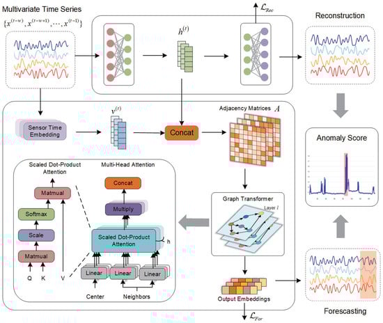
Figure 1.
Overall framework of SGTrans. The overall framework of the SGTrans model involves three parts: Sparse Autoencoder module, Graph Transformer Forecasting Module, Joint Optimization, and Anomaly Score.
- (1)
- Sparse Autoencoder Module. It aims to reduce and reconstruct the high-dimensional sensor time series data, and obtain more meaningful hidden representations.
- (2)
- Graph Transformer Forecasting Module. It models the global temporal dependencies of time series, in which the Sensor Time Embedding layer, Graph Structure Learning, Graph Transformer Feature Extractor, and Output Layer, respectively, are designed to make the proposed framework explicitly learn more comprehensive dependencies between sensors.
- (3)
- Joint Optimization and Anomaly Score. SGTrans combines the reconstruction error and forecasting error to calculate the abnormal score to determine the occurrence of abnormal events.
3.3. Sparse Autoencoder Module
In real-world industrial IoT environments, sensor-generated data typically exhibit high dimensionality and include noise and irrelevant information due to the high variability in operating conditions. These characteristics are detrimental to subsequent data analysis and modeling. In this study, a Sparse Autoencoder (SAE) reconstruction module is employed to process multivariate time series data produced by sensors. This module can learn sparse representations from high-dimensional time series to capture the most informative key features and suppress less correlated noise features. These sparse latent features are input into the SAE decoder for reconstruction, and are used as inputs for a subsequent Graph Transformer network to predict future behaviors.
SAE primarily utilizes an encoder–decoder network to learn efficient representations of input data. The input datum is compressed by the encoder into a sparse latent representation h in the hidden layer, which is subsequently reconstructed into the output datum by the decoder. To control the sparsity of the learned latent features, the SAE incorporates a sparsity constraint that limits the number of active neurons in the hidden layer (a neuron output close to 1 indicates that it is active, and close to 0, inactive). This constraint is primarily achieved by introducing a sparsity parameter, , which satisfies the following properties:
where denotes the activation value of m-th neuron in the hidden layer for input x, and denotes the actual average activation value of the m-th neuron in the hidden layer. To induce sparsity in the latent features obtained by the hidden layer, it is desirable for the average activation value to be close to 0. This constraint aims to force the majority of hidden neurons to remain inactive, allowing only a few neurons to be active. These active neurons can then capture the most representative features. Such sparsity constraints ensure that the sparse latent features obtained by the hidden layer can automatically learn important features while filtering out noise and unimportant information in the data.
The objective of SAE is to ensure that the reconstructed output closely approximates its input, while limiting the activation to a few neurons that are tasked with learning the most representative sparse latent representations, that is, to simultaneously minimize the reconstruction error and the difference between and . Therefore, the loss function of the SAE reconstruction module comprises the reconstruction error and a sparsity constraint, enforced through a penalty based on Kullback–Leibler (KL) divergence as follows:
where is the reconstruction error term, denoting the mean square error (MSE) between the original data x and the reconstructed data , represents the penalty coefficient, and M represents the size of the neurons in the hidden layer. The KL divergence penalty is used for quantifying the disparity between and , controlling the sparsity of hidden features.
3.4. Graph Transformer Forecasting Module
3.4.1. Sensor Time Embedding
CPS sensors are commonly classified and grouped according to their respective functionalities. Using a water treatment facility as an example, the water treatment process includes several stages, such as raw water storage and chemical pretreatment. There exists a correlation between sensors in different treatment processes. Furthermore, sensors within the same process also display strong internal associations. To gain a deeper comprehension of this sensor data, we assign a randomly generated embedding vector to every individual sensor node. Then, is input into the Transformer network to capture the time-dependent relationships among sensors within the same process p, defined as follows:
where denotes the process of Transformer processing for all sensors in the process p. Transformer is chosen primarily because of its capability for parallel processing and efficiency.
3.4.2. Graph Structure Learning
Each sensor in CPS usually exhibits different characteristics, with complex topological associations between them. Therefore, we tend to use graph structure learning to capture the potential dependencies between each sensor. Considering N sensors, and that the dependency patterns among them are not necessarily symmetric, we use a directed graph , where node represents the timing embedding of each sensor, and denotes the relationship between different sensors. Specifically, we define an adjacency matrix . If there is a connection between node i and node j, then is marked as 1 and otherwise as 0. Assuming we have no prior information about the graph structure, the candidate relationship set that each node i depends on is , which is a set of sensor numbers that may have a dependency relationship with sensor i. Considering the large number of sensors, to prevent the generated graph from being too dense and thus causing high computational costs, we use the closest previous number of neighbors associated with each sensor i, controlling the sparsity of through the parameter k. The adjacency matrix can be constructed as follows:
where denotes the indicator function, and TopK denotes the k sensor indexes selected from the candidate relation set that are most similar to sensor i. denotes the normalized dot product between the sensor embedding of node i, and the candidate neighbor nodes j. Next, we introduce the feature extraction module based on Graph Transformer, which will use the aforementioned learned adjacency matrix A.
3.4.3. Graph Transformer Feature Extractor
Transformer originally made its mark in the NLP field and has achieved significant success in many NLP tasks. Similarly, Transformer-based models have demonstrated strong performance in multivariate time series anomaly detection, but these methods lack consideration for inter-series correlations. Recently, methods based on graph structure learning, such as GAT, have been proposed that explicitly capture the correlations between time series. However, these graph structure learning methods focus only on the features of nodes and their immediate neighbors, neglecting the utilization of edge features, which may result in insufficient capture of global dependencies. Therefore, we have designed a feature extraction module based on a multi-layer Graph Transformer network, incorporating Transformer’s multi-head attention mechanism into graph structure learning and integrating edge features. Each attention head focuses on different aspects, enabling a more comprehensive modeling of the relationships between nodes in the graph.
Assume denotes the node features of Graph Transformer at time t for layer l. To mitigate the noise impact on Graph Neural Networks and to imbue each node feature with richer temporal information, we use the sparse hidden feature generated by Sparse Autoencoder concatenated with the sensor time embedding as the initial input, denoted as , where denotes the trainable weight parameter matrix of the input. Simultaneously, the inherent correlation between node i and node j is integrated, serving as the edge feature representation. We calculate the multi-head attention from node j and node i, as follows:
where denotes exponential scale dot-product function, d represents the hidden size of each attention head, the neighbor set of node i. In each attention head, trainable parameters are employed to map node feature to query vector , and are used to map to key vector . The edge feature acts as additional information to enhance the association between two nodes, which is encoded by and added to the key vector. These feature vectors collectively contribute to calculating multi-head attention coefficients between node i and node j at every layer.
After obtaining the graph multi-head attention, we aggregate information from all neighboring nodes j to node i. This yields the comprehensive aggregated feature, , for node i, as follows:
where is a trainable parameter that transforms the features of node j into . denotes the concatenation operation of C head attention. Compared with GAT, which uses a normalized adjacency matrix as the transition matrix for message passing, Equation (13) substitutes this with a multi-head attention matrix. This multi-head attention matrix enables us to weigh and aggregate information according to the relationship between nodes and additional edge features, obtaining a richer representation of each node feature.
3.4.4. Output Layer
The features extracted by the Graph Transformer layer, denoted as , are scaled by the sensor time embedding and then passed into a linear layer for final prediction. The sensor prediction value of time step t is obtained:
where ∘ denotes element-wise multiplication. Lastly, we utilize the Mean Squared Error (MSE) between the predicted sensor behavior data and the actual observed data as the loss function for our forecasting model:
3.5. Joint Optimization and Anomaly Score
3.5.1. Joint Optimization
Our SGTrans model combines the advantages of both the reconstruction and forecasting modules. The reconstruction module captures the data distribution of the original input, obtaining superior sparse hidden representations, while the forecasting module forecasts the observations for the next timestamp. During the training process, the SAE-based reconstruction task and the Graph Transformer-based forecasting task are jointly optimized. The loss function contains two optimization objectives, namely, the reconstruction loss and the forecasting loss, defined as follows:
where denotes a hyper-parameter ranging between 0 and 1, used to balance the reconstruction and forecasting model.
3.5.2. Anomaly Score
The anomaly score for sensor node i at time t is calculated as follows:
where denotes the mean square error of the predicted time series value for the sensor node i at time t, and denotes the mean square error of the reconstructed time series value. To mitigate potential inaccuracies caused by either the reconstruction or forecasting model, we employ the Weighted Harmonic Mean (WHM) to balance the influence of errors from both models. Specifically, we calculate the weighted harmonic mean of reconstruction and forecasting errors using the weight factor defined in Equation (16), which serves as the final anomaly score for each sensor time series. If exceeds the set anomaly threshold, we label the time series window at timestamp t as an anomaly. We use extreme value theory [] to determine the anomaly threshold in this context.
4. Experiments
4.1. Datasets
We adopt three real-world benchmark datasets to evaluate our time series anomaly detection method. These datasets include SWaT [], WADI [], and SMAP [], with detailed statistics presented in Table 1. The SWaT and WADI are datasets published by the Trust Center, primarily used for cybersecurity and industrial control system security research. The SMAP dataset originates from NASA’s satellite missions and contains time series data on soil moisture and the Mars Science Laboratory experiments. Each dataset consists of a set of normal data samples for training and an independent test set containing both normal and abnormal samples, serving to assess the performance of our anomaly detection methods. We downsample the raw data from the SWaT and WADI datasets to capture measurements every 10 s, and we normalize the data during preprocessing to enhance consistency and comparability.

Table 1.
Statistical summary of real-world datasets.
4.2. Baselines and Evaluation Metrics
We use eight benchmark methods for the comparison and evaluation of multivariate time series anomaly detection, including PCA, AE, DAGMM [], LSTM-VAE [], MAD-GAN [], USAD [], GDN [], and TranAD []. PCA, AE, and DAGMM are three simple traditional baseline methods, while the others are more advanced algorithms proposed in recent years. The details are as follows:
DAGMM: Deep autoencoding and Gaussian mixture model are combined to generate low-dimensional feature representations of the data, with the reconstruction error serving as the metric for anomaly evaluation.
LSTM-VAE: LSTM-VAE adopts LSTM to capture temporal dependencies and integrates with variational autoencoder to generate hidden space representations of data for anomaly detection.
MAD-GAN: GAN and LSTM-RNN are used as the generator and the discriminator, respectively, training both to capture the differences between normal and anomalous data.
USAD: Unsupervised anomaly detection trains with an autoencoder to learn low-dimensional representation of data, and adversarial training is used to improve anomaly detection performance.
GDN: A graph attention mechanism is used to learn the structural relationship between high-dimensional time series data, and the attention weight is used to explain the detected anomalies.
TranAD: Transformer Networks for Anomaly Detection is a forecasting-based anomaly detection method and uses attention-based sequence encoders for fast reasoning. Adaptive and adversarial training based on focus scores are used to improve the stability of anomaly detection.
In order to evaluate the performance of our method and baseline model, we select precision (P), recall (R), and F1-score (F1) as metrics. Precision is defined as the ratio of correctly detected anomalies to the number of samples labeled as anomalies. Recall measures the ratio of correctly detected anomalies to the total number of actual anomalies. The F1-score, which comprehensively considers both precision and recall, is defined as follows:
where , , and denote the true positive, false positive, and false negative, respectively.
4.3. Experimental Setup
Our proposed method is implemented using PyTorch 1.7.1 and is trained on a server equipped with an Intel(R) Core(TM) i9-11900K CPU @ 3.50 GHz and an NVIDIA RTX 3090 GPU. We use Adam optimizer for training with a learning rate of 0.0005, trained for 30 epochs. For SWaT, WADI, and SMAP, the dimensions of the sensor time embedding and the hidden layer size of the graph-based forecasting model are set to 16, 32, and 64, respectively; the number of nodes k in the adjacency matrix are set to 10, 20, and 15, respectively; and the weight factors are set to 0.5, 0.3, and 0.5, respectively. The sparsity constraint in SAE is set to 0.0001, the weight of the KL-divergence term is set to 1.0, the time window w is set to 16, and the batch size is set to 64.
4.4. Results and Analysis
Table 2 presents the comparison results for the precision, recall, and F1-scores of our model and all baseline models. It can be observed that our proposed SGTrans outperforms all baseline methods in terms of the F1-score metric on three public real CPS datasets: SWaT, WADI, and SMAP. Upon comparison, it is evident that most baseline methods show a lower F1-score on SWaT and WADI datasets. This is likely because these datasets contain data from more complex processes and abnormal situations. However, SGTrans still achieves the best results in F1-score, which are 1.61% and 5.32% higher than the best baselines, respectively, and also outperforms all baselines regarding recall. Furthermore, most baseline methods perform well on the SMAP dataset because they have relatively simple anomaly patterns, and SGTrans manages to exceed the best baseline in the F1-score by 1.34% on this dataset. Hence, by integrating the strengths of the Graph Neural Network and Transformer, and introducing the multi-head attention mechanism into graph structure learning for node information propagation, SGTrans effectively models the complex relationships and global temporal dependencies between sensor nodes, which is significant for anomaly detection.
Table 2.
Comparison with baseline methods in terms of precision, recall, and F1-score on SWaT, WADI, and SMAP. The best performances are highlighted in bold.
From the analysis of the results from various baseline methods, it is evident that traditional foundational algorithms like PCA and DAGMM underperform. This is primarily because they struggle to encode the comprehensive information within time series and lack a thorough consideration of global temporal dependencies. In addition, GDN and TranAD proposed in the past two years have also achieved better performance than other baselines. Despite this, GDN struggles to extract temporal features from time series, whereas TranAD ignores the spatial topological relationship between sensor data, which can be problematic in intricate sensor networks. Our proposed SGTrans outperforms both GDN, which solely employs the Graph Neural Network, and TranAD, which exclusively utilizes Transformer. This indicates the efficacy of integrating Graph Neural Networks with Transformers in multivariate time series anomaly detection.
4.5. Ablation Studies
To evaluate the impact of each component within our model, we conducted ablation experiments on the SWaT dataset. We tested four scenarios:
- (1)
- w/o SAE: SGTrans without Sparse Autoencoder. We remove the SAE reconstruction module.
- (2)
- w/o STE: SGTrans without Sensor Time Embedding. We remove the sensor timing embedding layer, and each sensor is substituted with a randomly initialized embedding vector.
- (3)
- w/o Transformer: SGTrans without Transformer. We remove the multi-head attention mechanism in the Transformer and replace it with the same weight assigned to each neighbor to aggregate information.
The results of the ablation study are summarized in Table 3. We can observe the following: (1) Removing the Sparse Autoencoder reconstruction module results in decreased detection performance. This suggests that dimensionality reduction and reconstruction processing for high-dimensional sensor time series data aid in obtaining more meaningful hidden representations of sensor nodes, subsequently enhancing the performance of anomaly detection to a certain extent. (2) Compared to the SGTrans model processed with the Sensor Time Embedding layer, the variant without this layer exhibits slightly inferior performance. This underscores the importance of embedding temporal information in the initial representations of sensor nodes. (3) The variant without the multi-head attention mechanism from the Transformer demonstrates the poorest performance. This is attributed to each univariate time series possessing distinctly different characteristics. Assigning equal weights to each neighboring node may introduce additional noise, rendering the model unable to effectively capture the intricate relationships and global temporal dependencies present in sensor time series data. In summary, the removal of any component leads to a performance decline, validating the rationale behind each component in SGTrans.
Table 3.
Performance comparison in terms of precision, recall, and F1-score of SGTrans and its ablated versions on SWaT. The best performances are highlighted in bold.
4.6. Effect of Hyper-Parameters
In this section, we explore the impact of three key hyper-parameters on our proposed SGTrans model: the number of nodes considered for the adjacency matrices k, the length of the time window w, and the weight factor balancing the reconstruction model and the prediction model. We conduct a sensitivity analysis on the SWaT dataset as shown in Figure 2.
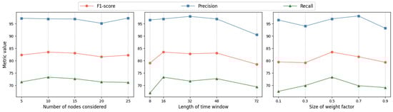
Figure 2.
Evaluation of hyper-parameter impact.
- (1)
- Number of nodes considered: The model’s performance is generally consistent across the set values, achieving optimal results when set to 10. To optimize computational efficiency, we set it to 10.
- (2)
- Length of time window: Performance degrades when the window is either too small or too large. A small window fails to adequately represent local contextual information. However, if the window is too large, short-term anomalies may be obscured among a large number of data points. The F1-score is better when the window size is set to 16, which is used in our experiments.
- (3)
- Size of weight factor: When set at 0.5, the performance is almost the best, with nearly equal contributions from the prediction-based and reconstruction-based models, resulting in a balanced final anomaly score.
4.7. Scalability and Efficiency Analysis
Experiments were conducted using the SWaT dataset to assess model training time and GPU memory usage across varying dataset sizes. Random continuous subsamples of 20%, 40%, 60%, 80%, and 100% of the dataset were used as training sets for experiments. The results, as shown in Figure 3, display the average training time per epoch, GPU memory usage, and F1-score trends with varying proportions of training data. It was observed that an increase in dataset proportion resulted in elevated training times and resource consumption per epoch, while the F1-score demonstrated an initial increase followed by a stabilization. These observations suggest that our model effectively balances dataset scale and performance. Practical applications can benefit from optimized training strategies to reduce runtime and resource consumption.
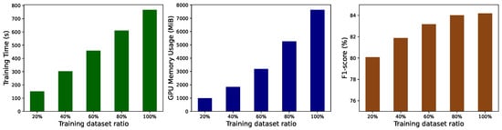
Figure 3.
Average training time per epoch, GPU memory usage and F1-score with dataset size.
4.8. Case Study
To further evaluate the effectiveness of our proposed model in real-world scenarios, we conducted a case study using the WADI dataset derived from a water distribution system, which includes actual attack scenarios. According to the attack description document in the WADI dataset, we selected the first documented anomalous period with a known cause for detailed analysis. This period was subjected to a persistent attack for up to 25 min, where the malicious behavior involved opening the motorized valve 1_MV_001_STATUS, leading to an overflow of the main water tank. Furthermore, the attacker skillfully manipulated the status of the motorized valve 1_MV_001_STATUS, ensuring it remained within normal range, making it challenging for human operators to detect the anomaly in time.
The dataset WADI simulates three subprocesses of the water distribution system: P1, P2, and P3. These subprocesses involve water inflow, taking water from P1 for distribution to users, and returning excess water to P1. Moreover, the system contains 127 sensors spread across the three subprocesses. The first number of each sensor name is used to identify the sub-process where the sensor is located. For example, the sensor 1_MV_001_STATUS is in P1. Within each subprocess, the sensors are intricately linked. If one subprocess experiences an attack or failure, it can trigger a chain reaction that impacts the operation of the entire system. Concerning the malicious act of opening the motorized valve 1_MV_001_STATUS, when the motorized valve 1_MV_001 that controls the water tank’s level is maliciously opened, it results in increased water flow and rising liquid levels in the tank. The change was detected by 1_FIT_001_PV, which measures the water flow, and 1_LT_001_PV, which monitors the water tank’s liquid level, so their readings correspondingly increased. However, this attack will not only affect the sub-process (P1) but also further affect the sub-process P2. Since the raw water from P1 is transferred to P2 through the transfer pump, the flow indicator transmitter 2_FIT_001_PV also showed an increase, and without doubt, the outlet pressure measured by 2_PIT_001_PV also changed. The anomaly scores of the attacked sensor and other sensors are affected by the attack as shown in Figure 4, which is consistent with ground truth operation logs. The comparison of sensor values predicted by our methods with the actual observations reveals that when one sensor is compromised, related sensors are affected, even if they are not directly attacked.
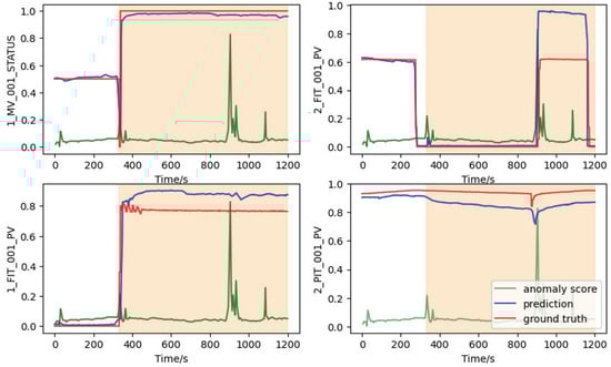
Figure 4.
The abnormalities of four related sensors during the attack period. The yellow area is the attack period.
The above case study analysis demonstrates that the SGTrans model can more fully capture sensor-dependent dependencies and effectively predict anomalies. This suggests that our model can promptly detect potential irregularities, providing crucial insights and guidance for daily operations.
5. Conclusions
In this work, we propose a novel anomaly detection framework SGTrans for the industrial field. The framework jointly trains a reconstruction module based on Sparse Autoencoder and a forecasting module based on the Graph Transformer network. Each module plays its distinctive role: the SAE effectively improves the high-dimensional and highly variable characteristics of sensor multivariate time series data. At the same time, the Graph Transformer network more comprehensively and explicitly models the temporal dependencies between sensor nodes in the graph structure to predict future behavior. Experimental results on multiple real-world datasets demonstrate that the SGTrans approach is superior to all baseline methods. Furthermore, we use a case study to illustrate this method’s application in real industrial scenarios. In the future, this method will be integrated with online learning to achieve dynamic anomaly detection. This will enable the method to handle ever-evolving data and environments to enhance practicality.
Author Contributions
Conceptualization, Q.Y., J.Z. (Jiaming Zhang) and S.L.; validation, Q.Y., J.Z. (Junjie Zhang) and C.S.; writing—original draft preparation, Q.Y.; writing—review and editing, Q.Y., Y.J. and S.X.; supervision, S.L. All authors have read and agreed to the published version of the manuscript.
Funding
This work was funded by the National Key R&D Program of China (2023YFB2904000, 2023YFB2904004), Jiangsu Key Development Planning Project (BE2023004-2), Natural Science Foundation of Jiangsu Province (Higher Education Institutions) (20KJA520001), The 14th Five-Year Plan project of Equipment Development Department (315107402), Jiangsu Hongxin Information Technology Co., Ltd. Project (JSSGS2301022EGN00), Future Network Scientific Research Fund Project (No. FNSRFP-2021-YB-15). Electric Power Research Institute of Electrical Guangdong Power Grid Co., Ltd. Project, Postgraduate Research Practice Innovation Program of Jiangsu Province (KYCX23_1084).
Data Availability Statement
This article makes use of public research datasets that are available from their respective authors using the links provided in the References section of this article.
Conflicts of Interest
Author Shanyi Xie was employed by the company Electric Power Research Institute of Electrical Guangdong Power Grid Co., Ltd. The remaining authors declare that the research was conducted in the absence of any commercial or financial relationships that could be construed as a potential conflict of interest.
References
- Wang, B.; Mao, Z. Detecting outliers in industrial systems using a hybrid ensemble scheme. Neural Comput. Appl. 2020, 32, 8047–8063. [Google Scholar] [CrossRef]
- Jeffrey, N.; Tan, Q.; Villar, J.R. Using Ensemble Learning for Anomaly Detection in Cyber–Physical Systems. Electronics 2024, 13, 1391. [Google Scholar] [CrossRef]
- Chang, C.C.; Lin, C.J. LIBSVM: A library for support vector machines. ACM Trans. Intell. Syst. Technol. TIST 2011, 2, 27. [Google Scholar] [CrossRef]
- Ramaswamy, S.; Rastogi, R.; Shim, K. Efficient algorithms for mining outliers from large data sets. In Proceedings of the 2000 ACM SIGMOD International Conference on Management of Data, Dallas, TX, USA, 15–18 May 2000; pp. 427–438. [Google Scholar]
- Jiang, L.; Xu, H.; Liu, J.; Shen, X.; Lu, S.; Shi, Z. Anomaly detection of industrial multi-sensor signals based on enhanced spatiotemporal features. Neural Comput. Appl. 2022, 34, 8465–8477. [Google Scholar] [CrossRef]
- Zong, B.; Song, Q.; Min, M.R.; Cheng, W.; Lumezanu, C.; Cho, D.; Chen, H. Deep autoencoding gaussian mixture model for unsupervised anomaly detection. In Proceedings of the International Conference on Learning Representations, Vancouver, BC, Canada, 30 April–3 May 2018. [Google Scholar]
- Li, D.; Chen, D.; Jin, B.; Shi, L.; Goh, J.; Ng, S.K. MAD-GAN: Multivariate anomaly detection for time series data with generative adversarial networks. In Proceedings of the International Conference on Artificial Neural Networks, Munich, Germany, 17–19 September 2019; Springer: Berlin/Heidelberg, Germany, 2019; pp. 703–716. [Google Scholar]
- Lin, S.; Clark, R.; Birke, R.; Schönborn, S.; Trigoni, N.; Roberts, S. Anomaly detection for time series using vae-lstm hybrid model. In Proceedings of the ICASSP 2020–2020 IEEE International Conference on Acoustics, Speech and Signal Processing (ICASSP), Barcelona, Spain, 4–8 May 2020; IEEE: Piscataway, NJ, USA, 2020; pp. 4322–4326. [Google Scholar]
- Liu, X.; Guo, J.; Qiao, P. A Context Awareness Hierarchical Attention Network for Next POI Recommendation in IoT Environment. Electronics 2022, 11, 3977. [Google Scholar] [CrossRef]
- Wu, F.; Souza, A.; Zhang, T.; Fifty, C.; Yu, T.; Weinberger, K. Simplifying graph convolutional networks. In Proceedings of the International Conference on Machine Learning, Long Beach, CA, USA, 9–15 June 2019; pp. 6861–6871. [Google Scholar]
- Wang, Y.; Sun, Y.; Liu, Z.; Sarma, S.E.; Bronstein, M.M.; Solomon, J.M. Dynamic graph cnn for learning on point clouds. ACM Trans. Graph. Tog 2019, 38, 146. [Google Scholar] [CrossRef]
- Ding, C.; Sun, S.; Zhao, J. MST-GAT: A multimodal spatial–temporal graph attention network for time series anomaly detection. Inf. Fusion 2023, 89, 527–536. [Google Scholar] [CrossRef]
- Deng, A.; Hooi, B. Graph neural network-based anomaly detection in multivariate time series. In Proceedings of the AAAI Conference on Artificial Intelligence, Virtual, 2–9 February 2021; Volume 35, pp. 4027–4035. [Google Scholar]
- Zhang, W.; Zhang, C.; Tsung, F. GRELEN: Multivariate Time Series Anomaly Detection from the Perspective of Graph Relational Learning. In Proceedings of the IJCAI, Vienna, Austria, 23–29 July 2022; pp. 2390–2397. [Google Scholar]
- Park, D.; Hoshi, Y.; Kemp, C.C. A multimodal anomaly detector for robot-assisted feeding using an lstm-based variational autoencoder. IEEE Robot. Autom. Lett. 2018, 3, 1544–1551. [Google Scholar] [CrossRef]
- Hundman, K.; Constantinou, V.; Laporte, C.; Colwell, I.; Soderstrom, T. Detecting spacecraft anomalies using lstms and nonparametric dynamic thresholding. In Proceedings of the 24th ACM SIGKDD International Conference on Knowledge Discovery & Data Mining, London, UK, 19–23 August 2018; pp. 387–395. [Google Scholar]
- Deldari, S.; Smith, D.V.; Xue, H.; Salim, F.D. Time series change point detection with self-supervised contrastive predictive coding. In Proceedings of the Web Conference 2021, Ljubljana, Slovenia, 19–23 April 2021; pp. 3124–3135. [Google Scholar]
- Devlin, J.; Chang, M.W.; Lee, K.; Toutanova, K. Bert: Pre-training of deep bidirectional transformers for language understanding. arXiv 2018, arXiv:1810.04805. [Google Scholar]
- Yu, C.; Wang, F.; Shao, Z.; Sun, T.; Wu, L.; Xu, Y. Dsformer: A double sampling transformer for multivariate time series long-term prediction. In Proceedings of the 32nd ACM International Conference on Information and Knowledge Management, Birmingham, UK, 21–25 October 2023; pp. 3062–3072. [Google Scholar]
- Zhang, Z.; Wang, X.; Gu, Y. Sageformer: Series-aware graph-enhanced transformers for multivariate time series forecasting. arXiv 2023, arXiv:2307.01616. [Google Scholar]
- Wu, S.; Xiao, X.; Ding, Q.; Zhao, P.; Wei, Y.; Huang, J. Adversarial sparse transformer for time series forecasting. Adv. Neural Inf. Process. Syst. 2020, 33, 17105–17115. [Google Scholar]
- Tuli, S.; Casale, G.; Jennings, N.R. Tranad: Deep transformer networks for anomaly detection in multivariate time series data. arXiv 2022, arXiv:2201.07284. [Google Scholar]
- Siffer, A.; Fouque, P.A.; Termier, A.; Largouet, C. Anomaly detection in streams with extreme value theory. In Proceedings of the 23rd ACM SIGKDD International Conference on Knowledge Discovery and Data Mining, Halifax, NS, Canada, 13–17 August 2017; pp. 1067–1075. [Google Scholar]
- Mathur, A.P.; Tippenhauer, N.O. SWaT: A water treatment testbed for research and training on ICS security. In Proceedings of the 2016 International Workshop on Cyber-Physical Systems for Smart Water Networks (CySWater), Vienna, Austria, 11 April 2016; IEEE: Piscataway, NJ, USA, 2016; pp. 31–36. [Google Scholar]
- Ahmed, C.M.; Palleti, V.R.; Mathur, A.P. WADI: A water distribution testbed for research in the design of secure cyber physical systems. In Proceedings of the 3rd International Workshop on Cyber-Physical Systems for Smart Water Networks, Pittsburgh, PA, USA, 21 April 2017; pp. 25–28. [Google Scholar]
- Audibert, J.; Michiardi, P.; Guyard, F.; Marti, S.; Zuluaga, M.A. Usad: Unsupervised anomaly detection on multivariate time series. In Proceedings of the 26th ACM SIGKDD International Conference on Knowledge Discovery & Data Mining, Virtual Event, CA, USA, 6–10 July 2020; pp. 3395–3404. [Google Scholar]
Disclaimer/Publisher’s Note: The statements, opinions and data contained in all publications are solely those of the individual author(s) and contributor(s) and not of MDPI and/or the editor(s). MDPI and/or the editor(s) disclaim responsibility for any injury to people or property resulting from any ideas, methods, instructions or products referred to in the content. |
© 2024 by the authors. Licensee MDPI, Basel, Switzerland. This article is an open access article distributed under the terms and conditions of the Creative Commons Attribution (CC BY) license (https://creativecommons.org/licenses/by/4.0/).