Abstract
We present SolarFlux Predictor, a novel deep-learning model designed to revolutionize photovoltaic (PV) power forecasting in South Korea. This model uses a self-attention-based temporal convolutional network (TCN) to process and predict PV outputs with high precision. We perform meticulous data preprocessing to ensure accurate data normalization and outlier rectification, which are vital for reliable PV power data analysis. The TCN layers are crucial for capturing temporal patterns in PV energy data; we complement them with the teacher forcing technique during the training phase to significantly enhance the sequence prediction accuracy. By optimizing hyperparameters with Optuna, we further improve the model’s performance. Our model incorporates multi-head self-attention mechanisms to focus on the most impactful temporal features, thereby improving forecasting accuracy. In validations against datasets from nine regions in South Korea, SolarFlux outperformed conventional methods. The results indicate that SolarFlux is a robust tool for optimizing PV systems’ management and operational efficiency and can contribute to South Korea’s pursuit of sustainable energy solutions.
1. Introduction
Solar energy is recognized as a renewable energy source with significant environmental benefits [1]. However, its role in a cost-effective energy strategy is limited by several factors. These challenges include its low power density and the large land area required for photovoltaic (PV) installations, which limits its capacity [2]. While PV installations continue to expand, underscoring the role of solar energy in the energy mix, it is important to consider the substantial and stable contributions of nuclear power, which is likely to remain a dominant energy source [3,4]. Furthermore, although PV panels are advertised to have a lifespan of approximately 25 years, practical experience often demonstrates a shorter lifespan, underscoring the necessity for a realistic assessment of the long-term viability of solar energy [5,6]. This context underscores the necessity for a diversified energy strategy that includes not only renewable sources such as solar but also the reliable capacity of nuclear power. In order to ensure a sustainable energy future, it is critical to improve the reliability and accuracy of solar PV power forecasting [7]. This forecasting will facilitate the integration of solar power into power grids, complementing stable sources such as nuclear power. Improved predictability enables the optimal integration of solar energy into the global energy mix, ensuring minimal environmental impact while meeting global demand.
Given the complex dynamics of integrating and increasing the penetration of solar power into electric grids, the inconsistent nature and periodic behavior of solar PV power prediction have become a critical issue [8]. Moreover, the accuracy of solar PV power prediction is strongly impacted by the meteorological and climatic variables of a given area, making predictions challenging [9]. In this light, very-short-term energy prediction can lead to improved operational scheduling of PV modules and enable proactive grid management, including safeguards against power fluctuations and emergency protocols for grid stability [10]. Yet, most standard solar energy forecasting methods have limited ability to discover correlations between small amounts of data; furthermore, they cannot explore such correlations and uncover implicit and relevant information about the solar energy system [11]. Therefore, many studies have investigated prediction methods for solar radiation, PV power generation, and other renewable energy sources [12]. To this end, researchers have used various modeling techniques to create an accurate model by combining various data [13]. However, some modeling approaches, such as linear or nonlinear regression models, may not be suitable for complex forecast tasks because of their processing costs [14]. Additionally, mathematical models cannot provide accurate results because they require many coefficients and sophisticated computations [15]. As a result, traditional methodologies cannot provide precise forecasts when dealing with the enormous volume of data generated by new power grids [16].
In light of these challenges related to solar power prediction, many recent studies have applied traditional machine learning (ML) models such as linear, nonlinear, and artificial intelligence models to renewable energy [17,18,19]. Qazi et al. [9] studied the application of artificial neural networks (ANNs) to perform modeling by using many weather features as inputs, resulting in a more accurate, dependable, and flexible network compared with that of other empirical models. Voyant et al. [20] applied ML algorithms to predict solar irradiation. They found that ML techniques such as nearest neighbor and bootstrap aggregation enhanced performance and accuracy. Almonacid et al. [21] investigated ANNs used to forecast the major parameters affecting the performance of high- and low-voltage solar PV systems. Wang et al. [22] used support vector machines (SVMs) and nonlinear time series to estimate the solar intensity. The SVM-based method achieved a low error rate, with kernel selection mainly based on experience. Tang et al. [23] used the least absolute shrinkage and selection operator (LASSO) and the single index model (SIM) to forecast solar intensity. However, simple ML approaches such as SVM, ANN, LASSO, and Ridge cannot provide high accuracy and are insufficient in scenarios with large amounts of data or the need to model the process of trends [1,8].
To overcome the limitations of traditional ML methods, some unique approaches, including deep learning (DL) algorithms, have been proposed [24]. DL algorithms are ANNs with a deep architecture that are capable of processing enormous amounts of data; they have outperformed state-of-the-art results in a variety of classification and regression tasks [25,26,27]. DL algorithms are expected to overcome the challenges posed by large-scale data [28]. Moreover, they can learn and discriminate features in a hierarchical way [19]. DL approaches have been applied to various domains of renewable energy and have provided higher forecast accuracy for wind and other renewable energies than traditional methods [19,28]. Recent studies have demonstrated the use of DL techniques and good ML tools for complex pattern detection, regression analysis, and forecasting [29]. DL techniques are becoming increasingly popular owing to their ability to identify relationships in time series data and easy applicability [30]. To further enhance performance, extra layers are added to the neural network (NN) architecture; this is called layering. Subsequently, numerous DL models have been developed, including Boltzmann machines, deep belief networks, and recurrent neural networks (RNNs) [31]. Boltzmann machines are a type of system that learns by making predictions about the future [32].
RNNs can be used to model time-dependent data, and they provide great results when applied to time-series data [33]. Long short-term memory (LSTM) is an advanced type of RNN that can retain information for significantly longer durations [34]. Therefore, it is extensively used for time series data forecasting, and it is particularly well adapted to solar PV power output forecasting. Studies have shown that DL-based NNs provide improved performance for time series prediction problems. For instance, LSTM NN and stacked autoencoders (SAEs) show superior performance when compared to some commonly used traditional prediction models [35]. Li et al. [36] applied both LSTM NN and SAEs to a prediction problem and found that the former had superior performance. By contrast, Patel [37] applied LSTM and a convolutional neural network (CNN) to solar radiation prediction and found that the model does not converge and does not provide satisfactory accuracy, with a high root mean square error (RMSE) value.
Prediction models must have high accuracy for renewable energy management, particularly for solar power generation. Hybrid DL models have emerged as a significant advancement in this field; they combine various DL approaches to enhance prediction accuracy [38,39,40]. This innovation addresses the limitations of existing sequential learning models, which struggle with incomplete data and fail to capture both spatial and temporal patterns effectively. An atrous convolutional layer (ACL) that extracts crucial features from data has been combined with a residual gated recurrent unit (RGRU) that learns spatial patterns within sequences to develop the ACL-RGRU model [41]. This model contributes toward optimizing renewable energy management systems by providing a comprehensive understanding of the spatiotemporal dynamics of data. Similarly, the GRU-CNN model adopts a two-step approach of initially analyzing temporal features using a GRU before incorporating spatial features through a CNN [42]. This model is adept at nonlinear mapping and extracting the intricate time series dynamics of PV power generation, and it offers insights into the complex atmospheric and meteorological conditions affecting solar power output. An echo state network (ESN) that offers nonlinear mapping ability has been combined with a CNN that offers spatial information modeling ability to develop the ESN-CNN model [43]. This model shows good efficiency and accuracy in renewable energy prediction, and it provides high performance on various evaluation metrics. The CNN-DeepESN structure excels at processing multidimensional data [44]. In this structure, CNN layers are used to extract spatial features, following which DeepESN layers are used to extract temporal features. It provides high-quality energy prediction, thus enhancing the reliability and efficiency of power systems and contributing to the integration of renewable energy sources into power grids.
Hybrid DL models, such as ACL-RGRU, GRU-CNN, ESN-CNN, and CNN-DeepESN, have significantly advanced the prediction of solar power generation. However, they exhibit considerable limitations in adapting to rapid, complex changes in solar energy data, often requiring extensive retraining when introduced to new geographic or climatic conditions. To overcome these challenges, we introduce the SolarFlux deep NN learning model, which not only enhances the accuracy of time series data forecasting for solar energy but also introduces innovative methodologies to the field. SolarFlux is based on temporal convolutional networks (TCNs) that excel at processing temporal information, and it incorporates dilated convolution and residual connections to expand the model’s receptive field. This approach effectively reduces the information loss and gradient decay issues commonly encountered in deep networks. Importantly, the utilization of Optuna for hyperparameter optimization is critical, as it systematically fine-tunes the model to optimize performance across diverse operational environments—a capability that markedly distinguishes SolarFlux from earlier models.
The main contribution of this paper are as follows:
- The empirical validation of SolarFlux at nine different PV sites in South Korea demonstrates its robustness and adaptability under a range of geographic and climatic conditions. This broad applicability is in stark contrast to previous models, which often underperform outside of their initial calibration settings.
- SolarFlux’s use of TCNs with advanced features such as dilated convolution and residual connections significantly improves the processing of temporal information. This methodological advance addresses and overcomes the long-term dependency challenges faced by models such as GRU-CNN and ESN-CNN, setting a new standard for DL in solar energy forecasting.
- By incorporating a self-attention mechanism and a temporal fusion transformer, SolarFlux achieves a dynamic and nuanced understanding of the interactions within the data. This capability is a significant leap forward from previous models that lacked the ability to dynamically adapt to the evolving patterns within complex sequence data.
- The strategic application of the teacher forcing technique and hyperparameter optimization using Optuna represents a pioneering approach in this field. These techniques not only enhance prediction accuracy but also significantly enhance the overall performance of SolarFlux, thereby establishing new benchmarks for efficiency and reliability in solar power forecasting.
The rest of this paper is organized as follows. Section 2 discusses the methodology and data used in the SolarFlux model. Section 3 presents the findings obtained by applying the model. Section 4 discusses the implications of these results, compares them with those of previous studies, and discusses potential limitations and areas for future research. Finally, Section 5 summarizes the main findings and contributions of this study and discusses future research directions.
2. Materials and Methods
2.1. Dataset Configuration
The decision to limit our investigation to South Korea is not merely a matter of convenience; it is a strategic choice based on the country’s distinctive geographical and climatic diversity. South Korea encompasses a diverse array of environments, including rugged inland terrains (e.g., Gwangju, Hadong, and Jinju), expansive coastal lines (e.g., Busan, Gangneung, Incheon, and Mokpo), isolated islands (e.g., Jeju), and other unique locations (e.g., Sejong). Each of these environments offers distinct data on solar energy dynamics. Moreover, the well-defined seasonal variations, ranging from cold, snowy winters to hot, humid summers, provide an invaluable framework for analyzing the efficacy and resilience of PV systems under varying meteorological conditions. These characteristics make South Korea an exemplary setting for studying solar energy dynamics, with findings that are relevant both locally and in similar climates worldwide [45]. Our methodology leverages South Korea’s geographical and climatic heterogeneity to explore essential questions about solar PV power generation efficiency and its environmental susceptibility. Through this approach, we aim to deliver original insights into optimizing PV systems for diverse global environments, significantly enriching the field of renewable energy research.
The experiments were conducted using publicly available PV performance data obtained from the Korean Open Data Portal (KODP) [46]. These data included measurements from multiple PV installations in different geographical locations, from inland to coastal and island areas within South Korea, collected at hourly resolution over a three-year period (2017–2019) [47]. The datasets included key meteorological factors known to affect PV performance, such as cloud cover, humidity, and solar irradiance. Temporal data, which are critical for the analysis of potential solar exposure, were represented by indicators such as month, day, and hour. This extensive dataset not only serves as the foundation for assessing PV power generation variability but also facilitates a detailed analysis of environmental impacts on energy production efficiency. Using this data, we demonstrate the effectiveness of our proposed forecasting model, focusing specifically on how solar radiation and other weather conditions influence PV power output. The meteorological data were sourced from the Korea Meteorological Administration (KMA) [48], providing detailed hourly records of weather conditions pertinent to solar power generation, including temperature, precipitation, humidity, sunshine duration, and solar irradiance.
Figure 1 presents a heatmap of the Pearson correlation coefficients, which assess linear relationships between variables across the datasets studied. This analysis helps quantify linear relationships specific to different regions, offering valuable insights into the dynamics of PV power generation and its influencing factors.
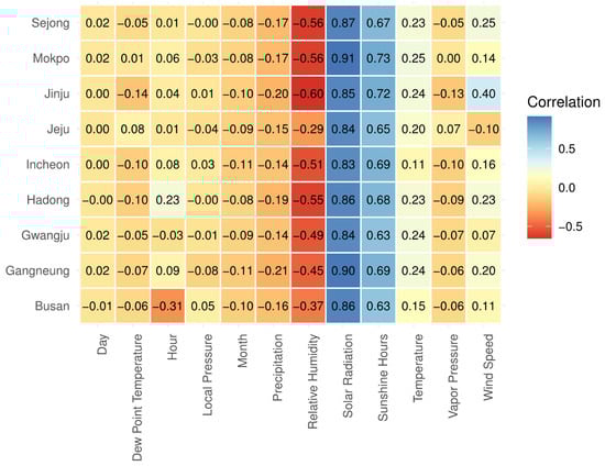
Figure 1.
Pearson correlation coefficient heatmap for nine regions in South Korea.
This analysis underscores that the significant relationships observed, such as the correlation between solar radiation and PV generation, are linear. However, it should be noted that other types of nonlinear correlations were not assessed in this study. Solar radiation exhibits a robust positive correlation with PV generation, with coefficients frequently exceeding 0.80. This suggests that PV generation is highly contingent on solar radiation. Similarly, sunshine hours and PV generation exhibit a positive correlation, with coefficients typically exceeding 0.60, indicating that PV generation is enhanced by clear weather conditions. In contrast, the correlation between temperature and PV generation is low, with coefficients ranging from 0.11 to 0.25. This indicates that temperature has a minimal effect on PV generation. In contrast, relative humidity has a strong negative correlation with PV generation, indicating that higher humidity levels lead to lower PV generation efficiency. The coefficients for this relationship range from −0.29 to −0.60. The observed variations in correlation coefficients across regions underscore the substantial impact of geographic and climatic conditions on solar power generation.
2.2. Model Construction
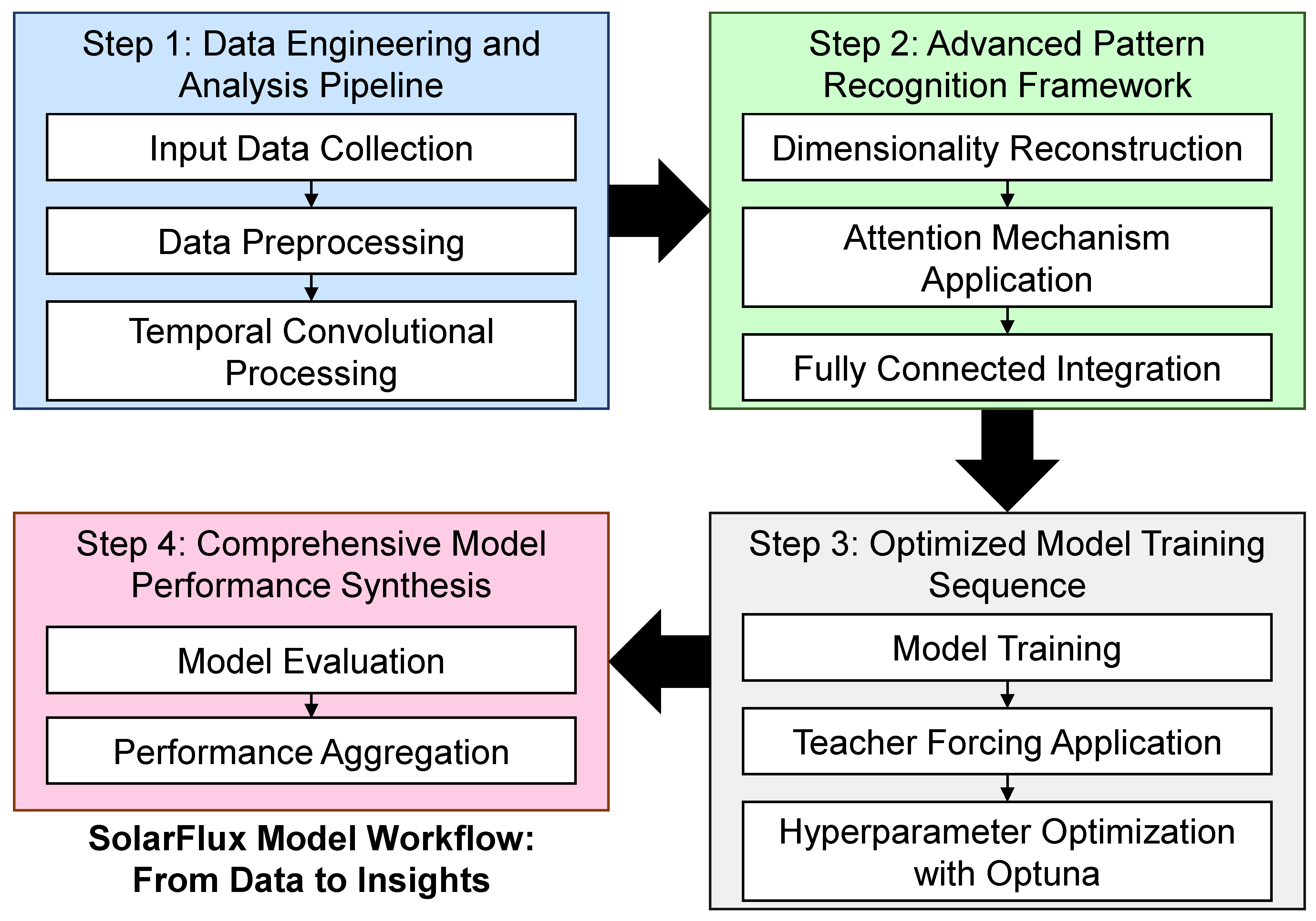
In this study, we proposed SolarFlux, a deep NN model designed to improve the prediction accuracy of time series data. SolarFlux utilizes TCNs, which efficiently process temporal information. The model incorporates dilated convolutions and residual connections to expand its receptive field, thereby reducing information loss and preventing gradient decay in deep networks. In addition, SolarFlux incorporates a self-attention mechanism that dynamically understands data interactions, allowing it to effectively handle complex sequence patterns through a temporal fusion transformer. Teacher forcing and hyperparameter optimization with Optuna are implemented to improve prediction accuracy and maximize the model’s performance. The overall structure of the SolarFlux model is illustrated in Figure 2.
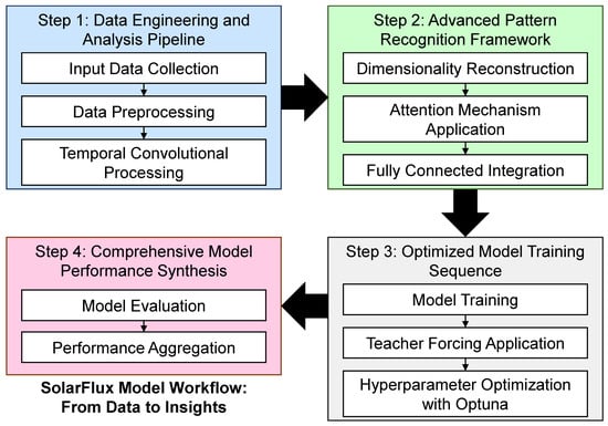
Figure 2.
Architecture of the SolarFlux model for multistep-ahead PV generation forecasting.
2.2.1. Temporal Convolutional Networks
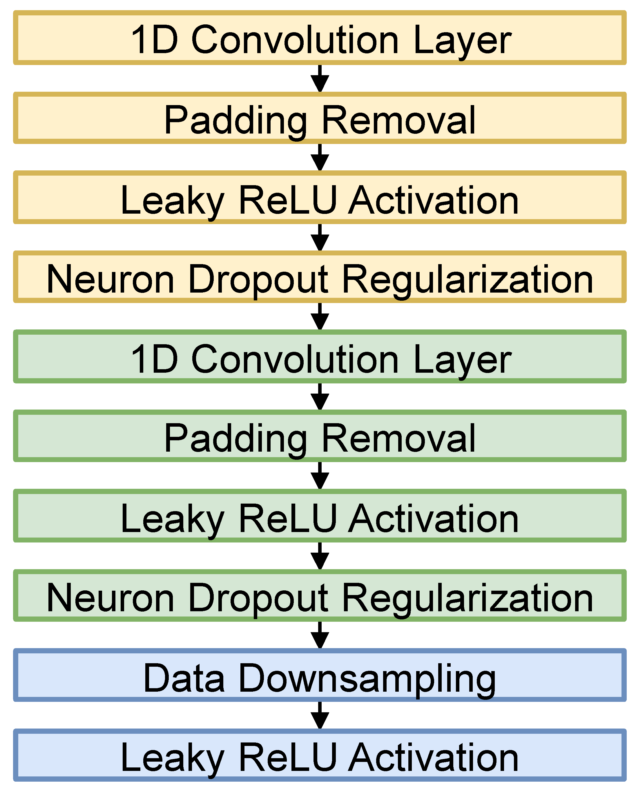
SolarFlux uses TCNs to capture the temporal characteristics of time series data and to efficiently model long-term dependencies. TCNs are characterized by their robust ability to process temporal information using a multilayer convolutional structure [49]. One of the distinctive features of TCNs is the use of dilated convolution, which introduces a fixed interval of dilation into the traditional convolutional operation, allowing the filter to sample the input data over a wider range [50]. This expands the receptive field of the model, allowing it to effectively learn from a longer range of information in the input sequence. In addition, the TCN structure includes residual connections, which add the input of each convolutional block directly to its output, preserving the input information as it passes through the network and enhancing the model’s learning ability [51]. The TCN model is constructed using the TemporalBlock as the basic unit, as shown in Figure 3.
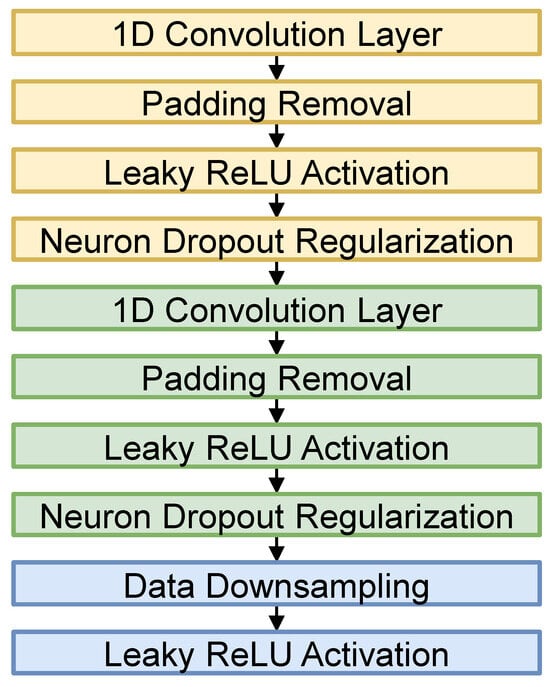
Figure 3.
Architecture of a temporal block.
Figure 3 illustrates the detailed setup of a TemporalBlock, where the first convolutional layer performs a dilated convolution and introduces nonlinearity through an activation function (LeakyReLU) and dropout to prevent overfitting. The second convolutional layer follows the same process, and the outputs of these two layers are combined with the input via residual concatenation. We integrate Equation (1) for the output of a dilated convolution operation as follows:
where y(t) is the output at time t; x(t) is the input signal; w(i) is the weight of the convolution filter at position i; N is the size of the convolution filter; and d is the dilation factor. This equation demonstrates how dilated convolutions allow the network to aggregate information over larger intervals without increasing computational complexity, thereby improving the model’s ability to capture long-term dependencies.
y(t) = sum (from i = 0 to N − 1) of [x(t − i × d) × w(i)],
2.2.2. Self-Attention Mechanism and Temporal Fusion Transformer
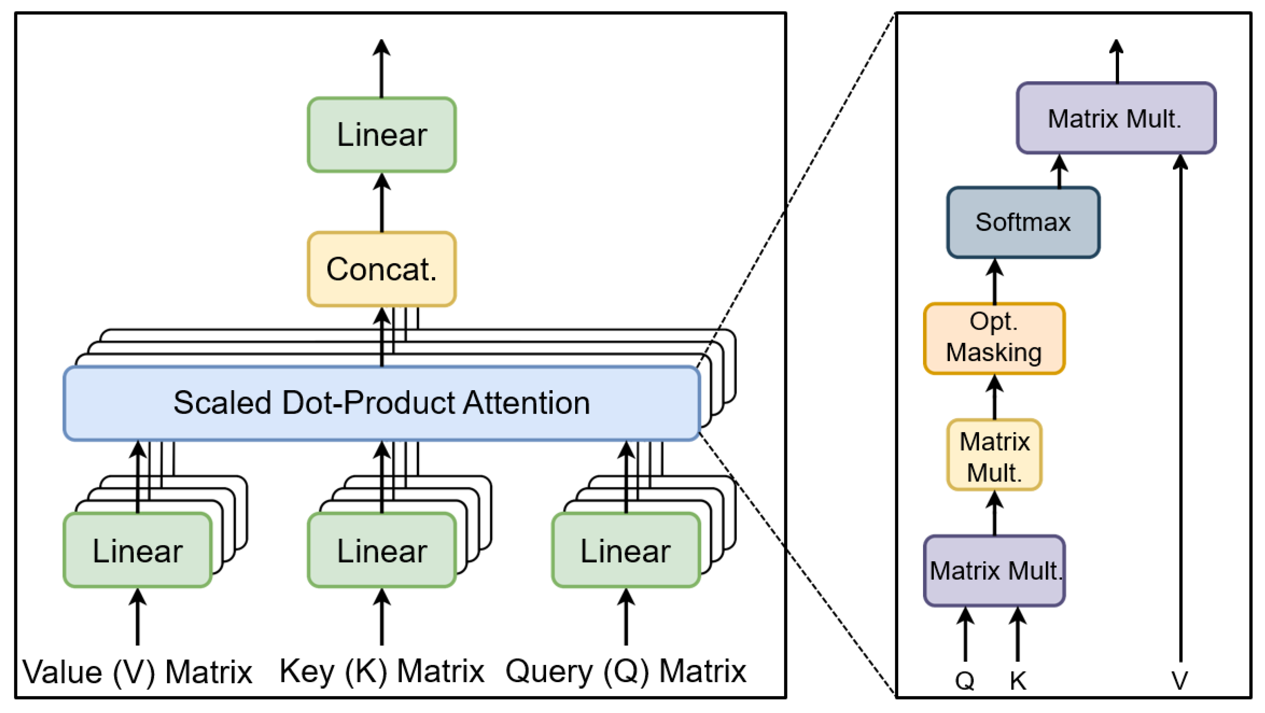
In this section, we introduce enhancements to SolarFlux through the integration of a self-attention mechanism and a temporal fusion transformer. These enhancements allow for a more precise analysis of features and interactions within sequence data. The self-attention mechanism dynamically determines the relevance of each data element, allowing the model to effectively focus on critical information. Building on this, the temporal fusion transformer optimizes the model’s handling of complex sequence patterns. Figure 4 depicts the architectural framework of a multi-head self-attention mechanism.
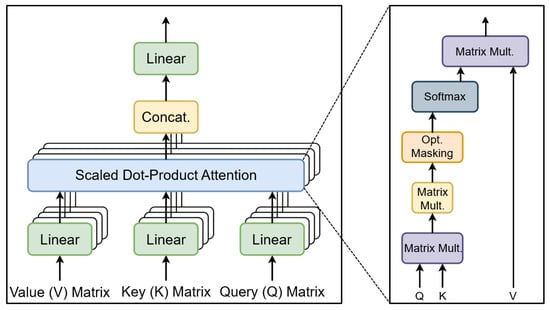
Figure 4.
Architecture of a multi-head self-attention mechanism.
The self-attention mechanism generates three distinct representations of each element within the input sequence: Query, key, and value [52]. These are used to compute the attention scores as follows: Each “Query” matrix Q is multiplied by the transpose of each “Key” matrix K and scaled by the inverse square root of dk, the dimension of the key vector. This process is crucial for comprehending the interaction depicted in Figure 4. The resulting matrix is then normalized using the softmax function, which computes the final attention scores. These scores reflect the significance of each element’s influence over others in the sequence. This calculation, as outlined in Equation (2), serves as the foundation for the weighted aggregation performed using the “Value” matrix V, resulting in the output that represents the attended features of the input sequence.
where Query, Key, and Value are matrices representing the query, key, and value vectors, respectively, for each element in the sequence. dk is the dimension of the key vector used for scaling. The softmax function is applied to normalize the scores, ensuring they sum up to 1, which allows them to be used as weights for the values.
Attention Score = softmax((Query × KeyT)/sqrt(dk)),
The self-attention component in SolarFlux is designed with multiple heads, allowing parallel processing across different data subspaces. This structure extends the model’s ability to analyze data from multiple perspectives simultaneously. The temporal fusion transformer combines a self-attention layer with a position-wise feed-forward network (FFN) [53]. In this setup, the self-attention layer examines the interactions between sequence elements, and the FFN applies nonlinear transformations independently at each position. These elements are integrated with layer normalization and residual connection to ensure that the learning process remains stable and effective, even in deep network architectures.
This architectural design incorporates sequential layers of TCNs and self-attention, where each layer processes the output of its predecessor, thereby enhancing the model’s ability to handle complex and diverse temporal patterns in sequence data. By integrating the self-attention mechanism and the temporal fusion transformer, we aim to significantly improve the performance of the model, specifically for solar PV power generation forecasting. This strategic enhancement allows the model to focus on important data elements and interpret complex dependencies with greater accuracy.
2.2.3. Enhanced Training Techniques for Accurate Time Series Prediction
We implemented three main strategies to improve the prediction accuracy and optimize the training process of the model. First, the multi-time step prediction method was used to enable the model to better recognize and interpret the evolving data patterns over time. Second, we used the teacher forcing technique to improve both the efficiency and accuracy of the learning process. Finally, learning rate scheduling was applied to accelerate learning initially and allow for precise fine-tuning in later stages, enabling both rapid learning in the early phases and meticulous adjustment during the subsequent phases. These integrated strategies significantly improve the learning capabilities and prediction performance of the model, especially in capturing the temporal dependencies and complex inherent patterns of time series data.
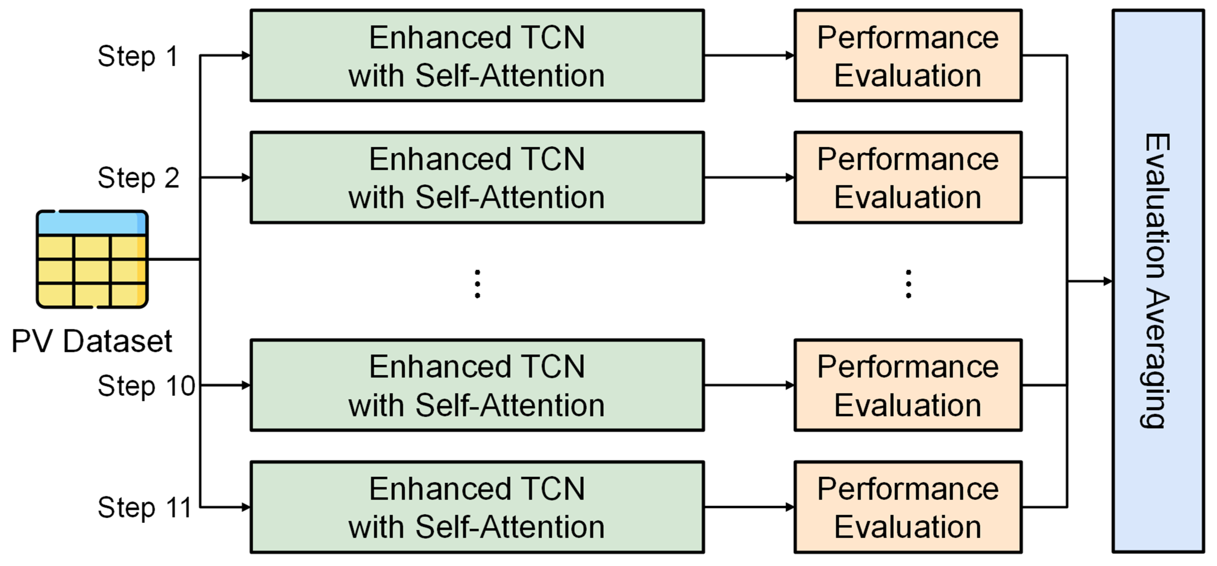
The multi-time step prediction method is critical in time series data analysis because it allows models to predict successive data points over multiple time points [54,55]. This method helps to effectively capture the continuity and complex dependencies of time series data. By predicting over multiple time steps, the model gains a deeper understanding of the dynamic changes and patterns, such as fluctuations in solar PV power generation, over time. In this study, forecasts were made for multiple time points from 8 a.m. to 6 p.m., tailored to the operational needs of the solar power industry, as depicted in Figure 5.
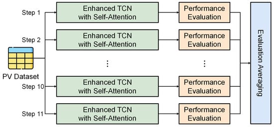
Figure 5.
Multistep-ahead PV generation forecasting process.
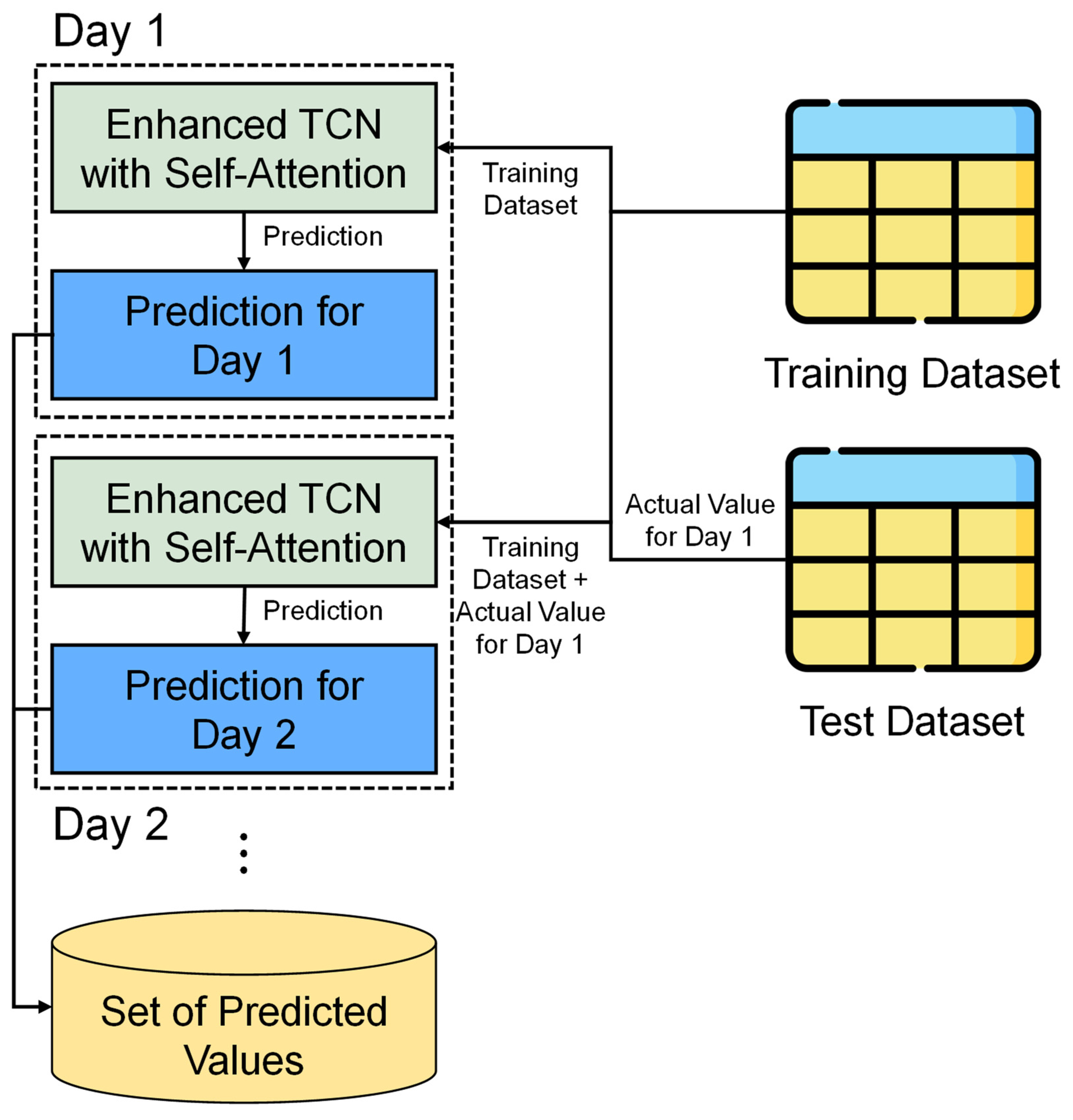
In addition, the teacher forcing technique, a validated approach for improving learning in neural network models dealing with sequential data, was implemented. This technique involves using the actual future output as a subsequent input during training, rather than the model’s own predictions. This technique aligns the model’s learning process more closely with real data distributions and prevents the propagation of errors throughout the learning process. This technique is demonstrated in Figure 6.

Figure 6.
Teacher forcing-enhanced prediction sequence process.
Finally, learning rate scheduling plays a pivotal role in the efficiency of training [56]. This technique involves initiating training with a higher learning rate to rapidly assimilate essential patterns and subsequently reducing it to refine and optimize the model’s performance. This adaptive approach benefits the model by stabilizing and refining learning, which is particularly advantageous when dealing with complex time series or high-dimensional datasets. This method provides a stable optimization path and enhances overall prediction accuracy.
2.2.4. Optuna for Hyperparameter Optimization
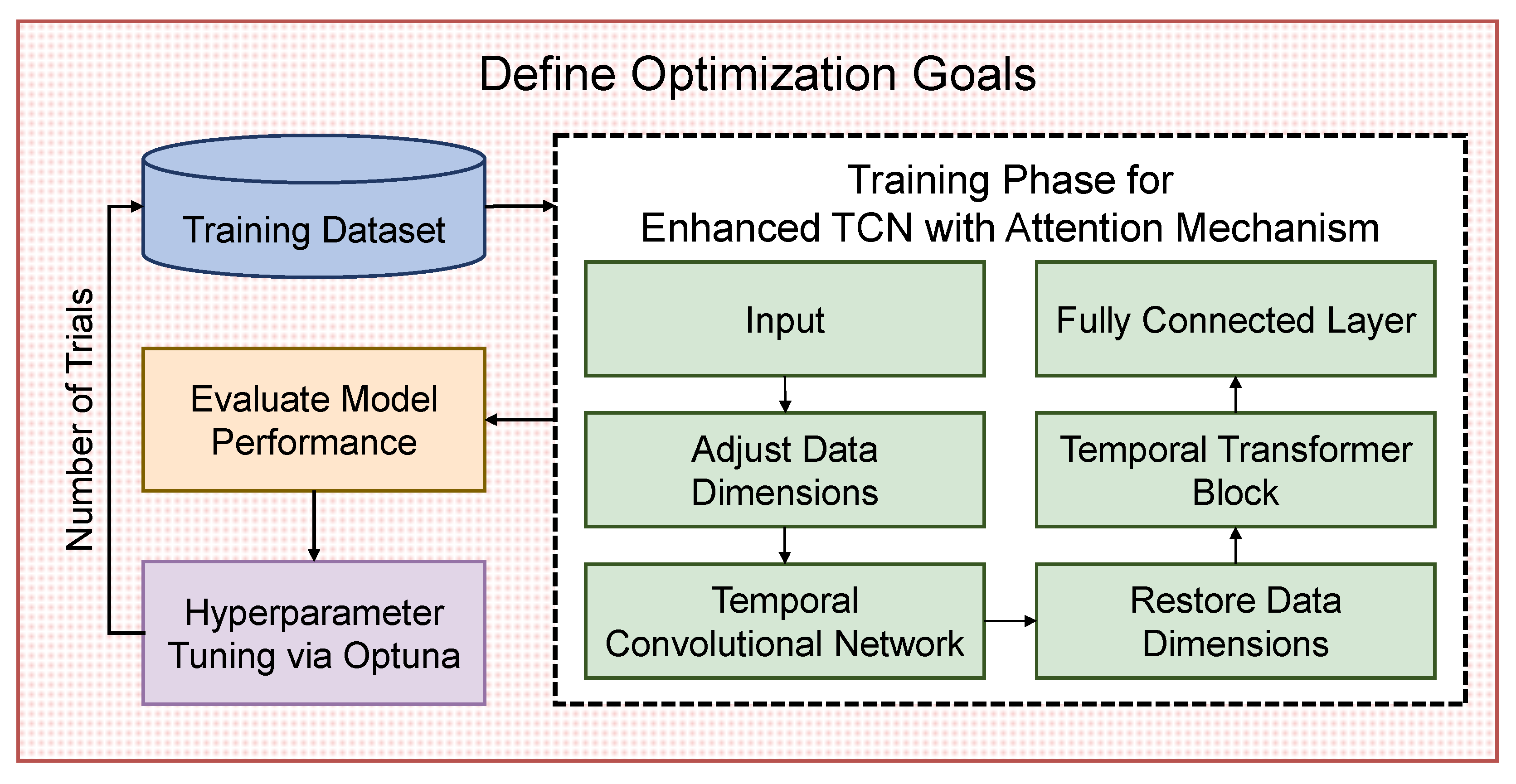
In order to enhance model performance in an efficient manner, this study employs the Optuna framework, which relies on Bayesian optimization principles. This approach helps identify the optimal combinations of the model’s crucial hyperparameters, streamlining the entire optimization process [57,58]. The hyperparameter optimization using Optuna is structured into four main steps.
In the first step, Optuna’s trial object is used to define the exploration domain for key hyperparameters that significantly affect model learning, such as the number of channels in the convolutional layer, learning rate, batch size, number of transformer layers, and forward expansion size. In the second step, the Optuna framework is used to construct the proposed model based on these hyperparameter combinations and train it using the training dataset. We then assess the effectiveness of each hyperparameter combination by evaluating the model’s performance on the validation dataset.
In the third step, the mean squared error (MSE) is used as the performance evaluation metric, with the goal of minimizing the MSE on the validation dataset. Optuna explores the hyperparameter space over a predefined number of trials, systematically refining the model settings. In the final step, the optimal set of hyperparameters determined by Optuna is used to reconstruct the TCN model and perform a final training on the full dataset to evaluate the generalization ability of the model. This optimization process is illustrated in Figure 7.
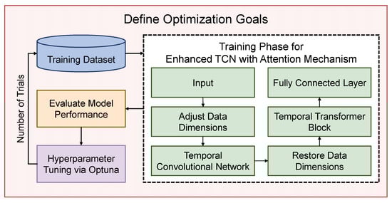
Figure 7.
Optuna-driven hyperparameter optimization process.
During the optimization process, the objective function O(H) that Optuna aims to minimize is defined, where H represents a set of hyperparameters, and it can be simplified as follows:
where MSEvalidation denotes the MSE on the validation dataset, and Model(H) signifies the model trained with the set of hyperparameters H. The ultimate goal is to identify the hyperparameter set H* that minimizes O(H), formulated as:
Objective function O(H) = MSEvalidation(Model(H)),
H* = arg min H O(H).
This approach ensures a systematic exploration and optimization of hyperparameters with the objective of achieving the best possible model performance on the validation dataset. This is subsequently verified on the complete dataset to assess the model’s generalization ability.
3. Results
We utilized data from nine regions in South Korea—Busan, Gangneung, Gwangju, Hadong, Incheon, Jeju, Jinju, Mokpo, and Sejong—to evaluate the performance of the proposed model. The training data span from 1 January 2017, at 08:00 to 31 December 2018, at 18:00. Predictions were subsequently performed for the year 2019, leveraging the insights gained from the training period. To ensure complete transparency and replicability of our research, comprehensive details of the hyperparameter settings employed across our models are meticulously documented in Appendix A.
3.1. Performance Evaluation Metrics
In this study, min-max normalization was adopted for preprocessing the data to evaluate the performance of the prediction model. It adjusts all data to a range between 0 and 1 and is used to ensure a consistent scale between model input data. Data normalization plays an important role in the selection of model performance evaluation metrics. In this study, we used the normalized root mean square error (NRMSE) and normalized mean absolute error (NMAE) as the main evaluation metrics. In addition, the coefficient of determination was used to evaluate the explanatory power of the model.
The NRMSE metric (Equation (5)) is normalized by squaring the difference between the predicted and actual values, averaging the squared and rooted values, and applying a ratio to the entire data range. It provides a measure of the magnitude of a model’s prediction error relative to the data range, thus providing a fair basis for comparing model performance on datasets of different scales.
The NMAE (Equation (6)) is a normalized metric that averages the absolute difference between the predicted and actual values. It represents the average prediction error of a model that is not affected by outliers. Applying the NMAE to data normalized by min–max normalization enables a consistent evaluation of the model’s performance.
where sqrt is the square root; sum, the summation symbol; yi, the actual values; yhati, the predicted values; n, the number of observations; mean(y), the mean of the actual values; and | |, the absolute value.
NRMSE = sqrt((1/n) × sum((yi − yhati)2))/mean(y) × 100,
NMAE = (1/n) × sum(|yi − yhati|)/mean(y) × 100,
In this study, min-max normalization is adopted as the preprocessing method. Therefore, the use of NRMSE and NMAE as the main performance evaluation metrics is reasonable for fairly and accurately evaluating the performance of the prediction model.
3.2. Comprehensive Ablation Study and Performance Analysis
The passage outlines the development of the SolarFlux model, designed to outperform traditional TCN frameworks as mentioned in [59,60,61]. It utilizes various TCNs, including standard, self-attention-based (SA-TCN), and multi-head self-attention (MHSA-TCN) models, to improve temporal pattern recognition. These TCNs process data more efficiently than RNNs and LSTMs, with enhancements such as self-attention mechanisms in SA-TCN and multiple attention heads in MHSA-TCN to capture complex data dependencies. Hyperparameters were optimized using the Optuna framework, as detailed in Appendix A. The model’s performance is quantitatively assessed in Table 1, which compares average NRMSE and NMAE across different regions.

Table 1.
Comparative analysis of average normalized root mean square error (NRMSE) and normalized mean absolute error (NMAE) for multistep-ahead predictions in each region, with mean values (left) and standard deviations (right, in parentheses).
This table covers one-step-ahead to 11-step-ahead predictions, clearly illustrating SolarFlux’s advanced capabilities in handling complex temporal data across diverse environmental conditions. Despite these enhancements, the data indicates that SolarFlux, with its distinctive integration of an MHSA-TCN, consistently outperforms both SA-TCN and MHSA-TCN across multiple regions. For instance, in Busan, SolarFlux exhibits a significantly lower average NRMSE of 40.85% and NMAE of 29.51%, in comparison to SA-TCN with an NRMSE of 83.12% and NMAE of 73.73%, and MHSA-TCN with an NRMSE of 81.66% and NMAE of 73.33%.
This superiority is in part attributable to the specialized workflow of SolarFlux, which includes advanced steps such as dimensionality reconstruction and attention mechanism application in its pattern recognition framework, followed by a comprehensive model training sequence involving teacher forcing and hyperparameter optimization with Optuna. SolarFlux is able to demonstrate its superiority by effectively incorporating advanced features that enhance both precision and reliability in predictions across diverse environmental conditions. This distinctive workflow not only enhances the accuracy of the predictions but also ensures that SolarFlux is adept at managing the complex variability typical of solar output in different geographic regions.
The Wilcoxon signed-rank test is a non-parametric statistical test employed to evaluate the discrepancy between two models and to ascertain whether that discrepancy is attributable to chance or is statistically significant [62]. This test considers both the magnitude and the sign of the observed difference in order to determine whether the difference between two models is statistically significant. In this instance, the significance level was set to 0.05. Table 2 presents the p-values of the Wilcoxon signed-rank test between SolarFlux and the other TCN models, based on the values of NRMSE and NMAE for one-step-ahead to 11-step-ahead forecasts for each model.
Table 2.
Results of the Wilcoxon signed-rank test between SolarFlux and other temporal convolutional network (TCN) models.
The difference in prediction performance between the SolarFlux model and other TCN models is not insignificant, but significant. The p-values obtained from the statistical validation results clearly show that SolarFlux is significantly better than other TCN models at the 0.05 significance level. For example, the p-values for NRMSE and NMAE between SolarFlux and other TCN models in different regions range from 0.00098 to 0.00293, indicating that SolarFlux outperforms other TCN models. These results clearly demonstrate the potential of SolarFlux as a powerful forecasting tool in the field of solar PV power generation forecasting.
3.3. Model Performance: Comparison with State-of-the-Art
The goal of this study is to compare the proposed model with a set of benchmark models, including LSTM, GRU, ACL-RGRU, GRU-CNN, ESN-CNN, and CNN-DeepESN, that have shown excellent performance in solar PV power generation forecasting. To create a comparable environment for multi-time step solar PV power generation forecasting, a multi-time step approach is used to organize the time steps from 1 to 11. The core structural framework of the benchmark models was followed as described in the research paper to design the models, and all benchmark models were tuned using Optuna to adjust hyperparameters to ensure optimal performance under the same experimental conditions.
LSTM is a type of RNN that specializes in learning the long-term dependence of time-varying data. It performs particularly well at predicting time series data, retaining important information, and eliminating unnecessary information through a gating mechanism that regulates the flow of information. LSTMs are used in a variety of fields, including electricity and solar energy forecasting, where they effectively learn patterns in complex time series data to provide high forecast accuracy. A gated recurrent unit (GRU) is a type of RNN designed to efficiently handle long-term dependencies in time series data. They offer similar performance to LSTMs despite their simple structure, and they use update gates and reset gates to regulate the flow of information. This model has been used in a variety of fields, including energy forecasting, natural language processing, and speech recognition, and it is widely used owing to its high learning speed and ability to effectively learn long-term dependencies.
ACL-RGRU [41] is a hybrid DL model for renewable energy forecasting that maximizes the efficiency of energy management through data preprocessing and accurate forecasting. The model extracts important features from data and learns temporal patterns to cope with the volatility of renewable energy, and it shows reliability. It also shows excellent performance in electricity and solar energy forecasting and application to smart grids. The GRU-CNN [42] model is a hybrid DL approach for solar power forecasting. It was developed by combining a GRU and a CNN. By simultaneously analyzing and predicting the temporal and spatial characteristics of solar power generation, the model significantly improves the accuracy of variable and intermittent solar power data. It can accurately model complex atmospheric conditions and meteorological variables, which is considered important for the efficient operation and management of energy systems.
The ESN-CNN [43] model provides a hybrid DL approach to improve the accuracy of renewable energy forecasting. By simultaneously analyzing the temporal variability and spatial characteristics of renewable energy, the model solves complex problems in energy forecasting, reducing computational complexity and reducing error rates. It plays an important role in power grid management and smart grid optimization, and its superiority has been demonstrated through various evaluation metrics. The CNN-DeepESN [44] model effectively learns complex temporal and spatial data patterns by extracting the spatial characteristics of solar power data with a CNN and processing the temporal dynamics with a DeepESN. It offers advantages such as improved prediction accuracy, reduced training complexity, and increased energy efficiency compared to those of traditional models, and it is useful not only for solar energy forecasting but also for a variety of time series and spatial data analysis tasks.
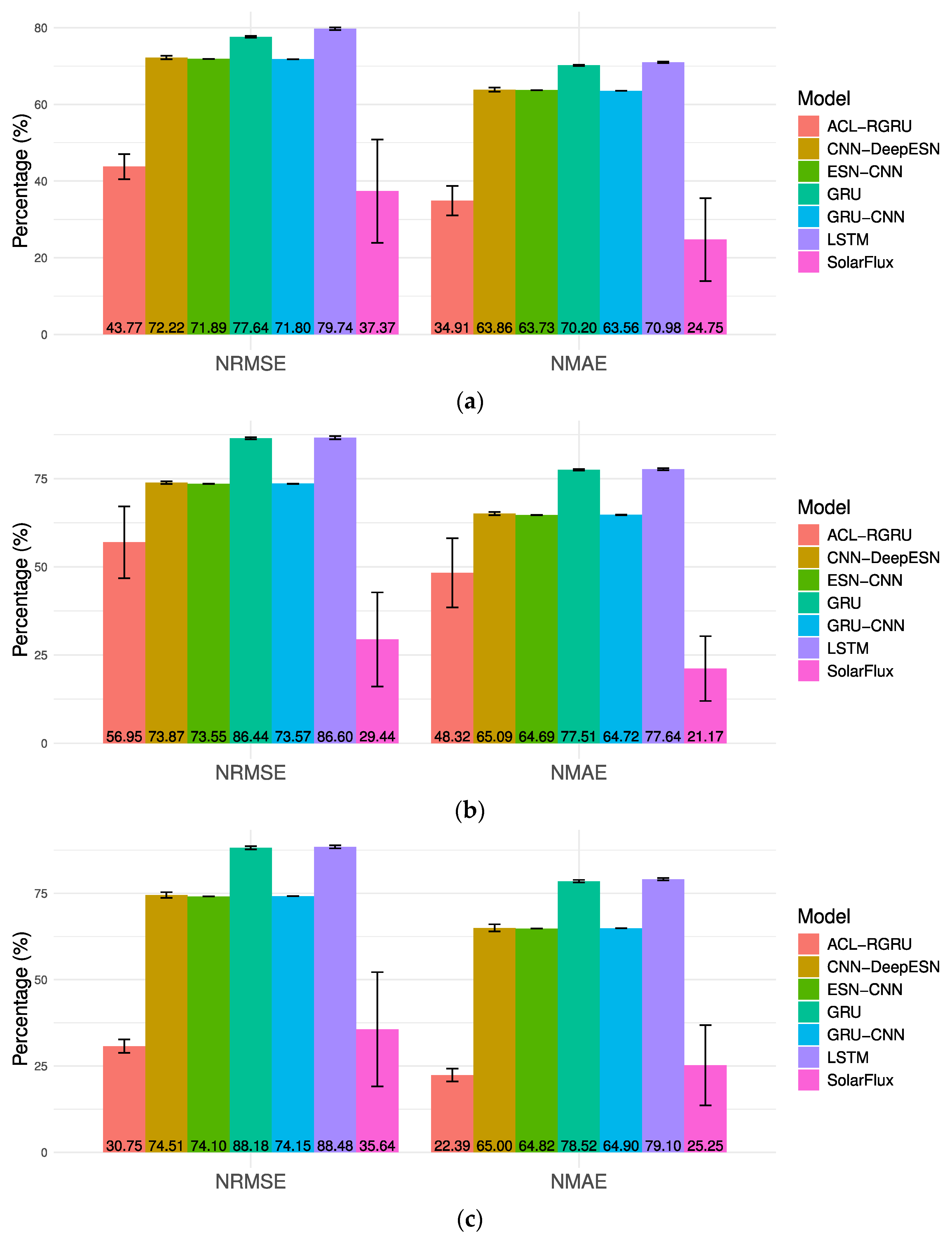
The analysis of the experimental results for the SolarFlux model, presented in Figure 8, Figure 9 and Figure 10, showcases the model’s predictive proficiency across various regions in South Korea. These results demonstrate the effectiveness of the SolarFlux model in forecasting PV power outputs and prove its robustness and accuracy over a range of conditions. SolarFlux shows a lower NRMSE and NMAE compared to those of other models. These metrics are crucial as they represent the difference between the predicted and actual values, with lower scores indicating higher accuracy.
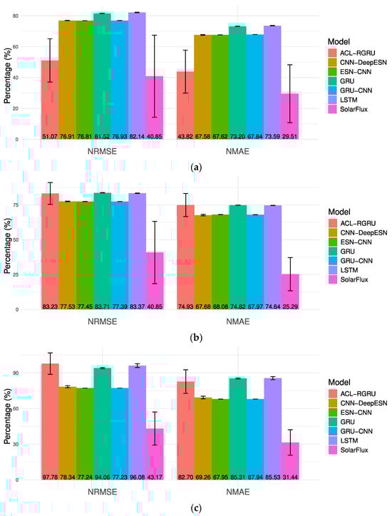
Figure 8.
Model performance over 1 to 11 steps with mean and standard deviation for normalized root mean square error (NRMSE) and normalized mean absolute error (NMAE). (a) Busan; (b) Gangneung; (c) Gwangju.
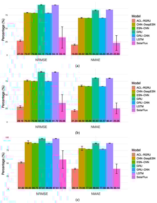
Figure 9.
Model performance over 1 to 11 steps with mean and standard deviation for NRMSE and NMAE. (a) Hadong; (b) Incheon; (c) Jeju.
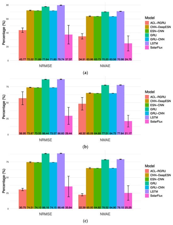
Figure 10.
Model performance over 1 to 11 steps with mean and standard deviation for NRMSE and NMAE. (a) Jinju; (b) Mokpo; (c) Sejong.
As illustrated in Figure 8, SolarFlux demonstrated superior performance in Busan, Gangneung, and Gwangju, consistently achieving the lowest NRMSE and NMAE values among all tested models. For example, in Busan, SolarFlux exhibited an average NRMSE of 40.85% and NMAE of 29.51%, which was considerably lower than that of the other models, including ACL-RGRU, which exhibited higher error rates of 52.79% NRMSE and 43.82% NMAE. This evidence demonstrates the efficacy of SolarFlux in effectively addressing the distinctive solar output variability characteristic of these regions’ environmental conditions.
As illustrated in Figure 9, SolarFlux exhibited commendable performance in the cities of Hadong and Incheon, although it was slightly outperformed by ACL-RGRU. For instance, in Incheon, SolarFlux exhibited an average NRMSE of 35.06% and NMAE of 25.05%, which were comparable to ACL-RGRU’s 28.21% NRMSE and 21.24% NMAE. This demonstrated a robust performance in a challenging environment with complex weather patterns. In Jeju, SolarFlux also demonstrated robust results, with an average NRMSE of 57.16% and NMAE of 39.90%. These figures were just behind those of ACL-RGRU, which had slightly better figures.
As illustrated in Figure 10, the SolarFlux model demonstrated superior performance in Jinju and Mokpo, outperforming all other models. In Jinju, the SolarFlux model achieved an average NRMSE of 37.37% and NMAE of 24.75%. In Mokpo, it led with an NRMSE of 29.44% and an NMAE of 21.17%. In Sejong, although not the leader, SolarFlux demonstrated competitive performance with an NRMSE of 35.64% and an NMAE of 25.25%. This was closely followed by ACL-RGRU, which recorded an NRMSE of 30.81% and an NMAE of 22.39%.
Across the nine datasets, SolarFlux demonstrated the highest performance in five regions, indicating its robustness and the effectiveness of its modeling approach. Notably, SolarFlux consistently achieved lower NRMSE and NMAE, demonstrating its capability to provide stable and reliable predictions across varied environmental and climatic conditions. These results underscore SolarFlux’s adaptability and precision in solar power generation forecasting, highlighting its potential as a valuable tool for optimizing solar energy utilization.
Table 3 provides a comprehensive illustration of the performance metrics of SolarFlux and other models, with averages and standard deviations calculated over nine distinct regions. This table offers a clear overview of the mean and standard deviations of NRMSE and NMAE for each model, emphasizing the superior stability and accuracy of SolarFlux. This results in an NRMSE of 39.18 with a standard deviation of 7.98, and an NMAE of 27.24 with a standard deviation of 5.68. This represents a significantly more stable prediction performance compared to ACL-RGRU, which has an NRMSE of 52.68 and an NMAE of 43.01. These figures demonstrate the robustness and versatility of SolarFlux across varied geographic and climatic conditions.
Table 3.
Average NRMSE and NMAE comparison across nine regions, with mean values (left) and standard deviations (right, in parentheses).
SolarFlux employs a self-attention-based TCN that enables it to efficiently discern patterns over time. This is particularly advantageous for time series forecasting of PV power outputs, where patterns can be complex and multifaceted. The utilization of multi-head self-attention mechanisms allows the model to prioritize critical temporal features and enhance prediction accuracy by focusing on the most significant data points. The application of the Optuna framework for hyperparameter optimization ensures that SolarFlux operates with an optimal configuration that significantly impacts its learning efficacy and generalization capabilities. SolarFlux could thus serve as a pivotal tool in the energy sector, particularly for regions transitioning to more sustainable energy sources.
4. Discussion
The proposed SolarFlux model is designed to improve the accuracy of time series data forecasting. SolarFlux is based on TCNs that are used to efficiently process temporal information and model long-term dependencies. The model uses dilated convolution and residual connections to reduce information loss and gradient vanishing problems that may occur in deep networks, and it introduces a self-attention mechanism and temporal fusion transformer to effectively handle complex patterns in sequence data. To improve the efficiency and prediction accuracy of the model, various strategies are applied, including multi-time step prediction, teacher forcing technique, and learning rate scheduling. In particular, hyperparameter optimization using Optuna plays an important role in maximizing the model’s performance. The performance of the SolarFlux model is validated by comparing it with several existing time series data prediction models.
The experimental results show that SolarFlux significantly outperforms various models such as LSTM, GRU, CNN-DeepESN, and ESN-CNN. In particular, the NRMSE and NMAE metrics of SolarFlux are significantly lower than those of other models. Compared with traditional NN models such as LSTM and GRU, SolarFlux showed lower errors, especially in terms of NRMSE and NMAE. This means that SolarFlux can better learn the complex patterns and dependencies of time series data and make more accurate predictions based on them. For example, the LSTM model showed NRMSE values that were approximately 2–3 times higher than those of SolarFlux, indicating that SolarFlux effectively captures the long-term dependence and temporal variability of the time series data. Compared to GRU, SolarFlux also outperformed on all metrics, suggesting that SolarFlux’s self-attention mechanism and temporal fusion transformer can overcome the shortcomings of GRU and better extract important information from sequence data.
Compared to CNN-DeepESN and ESN-CNN, SolarFlux achieved lower NRMSE and NMAE values. This shows that SolarFlux has a structure that can effectively handle the different characteristics of complex time-series data. In particular, the combination of temporal convolution and transformer-based structures enables excellent prediction performance. While the ACL-RGRU model performs well on datasets with certain conditions, its applicability and consistency are limited. ACL-RGRU primarily outperformed on datasets with scenarios in which short-term dependencies are more important. This suggests that ACL-RGRU specializes in capturing short-term patterns and volatility. By contrast, it often performed relatively poorly on datasets that contained long-term dependencies and complex sequence patterns, indicating that its structural limitations make it difficult to effectively model long-term dependencies. In comparison, SolarFlux maintains consistently high performance even on datasets where ACL-RGRU performs relatively poorly. This indicates that SolarFlux can comprehensively understand and handle a wide range of characteristics and dependencies in time series data.
5. Conclusions
In this study, we proposed SolarFlux, a sophisticated deep-learning model for PV power forecasting. Through experiments, we demonstrated its superior performance across various regions in South Korea. The experimental results demonstrated that SolarFlux exhibited a remarkable capacity to accurately predict PV outputs with robustness across different geographical and climatic conditions. For instance, in Busan, SolarFlux achieved an average NRMSE of 40.85% and NMAE of 29.51%, significantly outperforming other models such as ACL-RGRU, which recorded 52.79% NRMSE and 43.82% NMAE. Similarly, in regions such as Jinju and Mokpo, SolarFlux demonstrated superior performance, with an NRMSE of 37.37% and 29.44%, respectively. SolarFlux represents a significant advancement in the field of renewable energy management. It is a highly accurate tool for PV power forecasting that can contribute to the optimization of solar energy resources. Its development aligns with global sustainability goals and can significantly impact the operational efficiency of PV systems.
Notably, the robustness of SolarFlux was confirmed across nine distinct datasets, where it consistently demonstrated lower error rates in comparison to other models. This reinforces the effectiveness and validity of its modeling approach. Its development aligns with global sustainability goals and can significantly impact the operational efficiency of PV systems, promoting more reliable and effective energy solutions. As we continue to refine SolarFlux, it is poised to become an even more integral component in the advancement of renewable energy technologies. The application of SolarFlux to different countries with varying climatic profiles could enhance its generalizability and further confirm its effectiveness across diverse environments.
While SolarFlux has proven effective in our current studies, it has some limitations. The most significant of these is the extended training time due to the use of Optuna for hyperparameter optimization. While this process is beneficial for achieving high performance, it requires considerable computational resources and time, especially when searching for optimal configurations. Furthermore, the model’s reliance on historical data means that significant anomalies in the training data could impact its predictive accuracy. Moreover, the model’s complexity, while beneficial in handling diverse and complex data patterns, may limit its accessibility for some applications due to the high computational demands associated with its use.
Future research should concentrate on optimizing the hyperparameter tuning process in order to reduce training times without compromising performance. Furthermore, enhancing the model’s robustness against anomalous weather conditions could further improve its predictive accuracy, which is of crucial importance in the context of climate variability. The incorporation of real-time data assimilation could enable the model to adjust to unforeseen changes in weather patterns, potentially increasing its utility in dynamic environmental conditions. Moreover, the application of transfer learning techniques may permit SolarFlux to adapt more expeditiously to novel regions without the necessity for extensive retraining, thereby enhancing its scalability and generalizability. We anticipate that the augmented functionality will render SolarFlux a more versatile instrument in the global pursuit of efficient and sustainable energy solutions.
Author Contributions
Conceptualization, H.M.; methodology, H.M.; software, H.M., S.H. and J.S.; validation, S.H. and J.S.; formal analysis, H.M. and J.M.; investigation, B.S.; resources, H.M. and B.N.; data curation, J.M.; writing—original draft preparation, H.M.; writing—review and editing, B.N. and J.M.; visualization, H.M. and J.M.; supervision, B.N. and J.M.; project administration, B.N. and J.M.; funding acquisition, J.M. All authors have read and agreed to the published version of the manuscript.
Funding
This study was supported by the MSIT (Ministry of Science, ICT), Korea, under the National Program for Excellence in SW, supervised by the IITP (Institute of Information & communications Technology Planning & Evaluation) in 2021 (2021-0-01399) and the Soonchunhyang University Research Fund.
Data Availability Statement
Data supporting the results reported in this study are openly available at the Korea Open Data Portal (https://www.data.go.kr/en/index.do) (accessed on 25 May 2024) and the Korea Meteorological Administration Data Portal (https://data.kma.go.kr/resources/html/en/aowdp.html) (accessed on 25 May 2024).
Acknowledgments
The author wishes to thank Hwimyeong Ha of LG Energy Solution, Ltd., for his expert insights. His contributions were invaluable to the development and potential application of the technology discussed in this paper. We would also like to express our sincere gratitude to the four reviewers and editors for their insightful and valuable feedback, which has helped us improve our work.
Conflicts of Interest
The authors declare no conflict of interest.
Appendix A
In this study, we employed the Optuna framework for systematic hyperparameter tuning to optimize our LSTM/GRU and TCN models, focusing on minimizing the MSE across various trials. Below, we provide specific details regarding the hyperparameter ranges and critical aspects of the optimization process.
The LSTM/GRU model optimization involved tuning several key hyperparameters within predefined ranges:
- Hidden Size: We explored hidden sizes ranging from 16 to 128. This parameter is crucial as it determines the model’s ability to learn and represent complex data patterns.
- Number of Layers: We tested models with 1 to 3 layers. Adding layers can enhance the model’s ability to capture more abstract representations of the input data.
- Learning Rate: We used a logarithmic scale for the learning rate, from 1 × 10⁻⁵ to 1 × 10⁻¹. This range allows for fine-tuning the model’s learning process over epochs.
- Batch Size: We experimented with batch sizes from 32 to 256, which influences both training stability and computational load.
- Dropout was set at a fixed rate of 0.3 to mitigate overfitting, especially vital in complex models or smaller datasets.
For TCNs, the hyperparameter tuning was crucial for adapting the model to the temporal dynamics of the datasets:
- 6.
- Number of Layers: Configurations varied from 1 to 4 layers, allowing the network to learn complex temporal patterns at multiple scales.
- 7.
- Number of Channels: Channels per layer were set between 16 and 128, impacting the network’s depth and capacity.
- 8.
- Kernel Size: We chose kernel sizes from 2 to 8. This choice affects how the model aggregates information over time, crucial for capturing temporal dependencies.
- 9.
- Dropout Rate: We varied dropout between 0.1 and 0.5 to effectively manage overfitting across different model complexities.
- 10.
- Learning Rate: The learning rate was also tuned on a logarithmic scale from 1 × 10⁻⁵ to 1 × 10⁻¹, optimizing the speed and quality of model training.
Each trial within the Optuna framework involved:
- 11.
- Configuring the model with the trial’s suggested parameters.
- 12.
- Training the model on a designated training dataset.
- 13.
- Evaluating the model using MSE loss on a validation dataset.
The use of device-specific adaptations (e.g., ‘to(device)’) ensures that the models are compatible with different computational resources, such as GPUs or CPUs, enhancing the execution efficiency. This consideration is pivotal in reproducing the models under different hardware setups.
By presenting these details, we aim to provide a comprehensive guide that allows other researchers to replicate our models accurately. The explicit mention of hyperparameter ranges and model settings ensures that the experiments can be faithfully recreated, thereby contributing to the robustness and reliability of our research findings.
References
- Zameer, A.; Jaffar, F.; Shahid, F.; Muneeb, M.; Khan, R.; Nasir, R. Short-term solar energy forecasting: Integrated computational intelligence of LSTMs and GRU. PLoS ONE 2023, 18, e0285410. [Google Scholar] [CrossRef] [PubMed]
- Al-Shahri, O.A.; Ismail, F.B.; Hannan, M.A.; Lipu, M.S.H.; Al-Shetwi, A.Q.; Begum, R.A.; Al-Muhsen, N.F.O.; Soujeri, E. Solar photovoltaic energy optimization methods, challenges and issues: A comprehensive review. J. Clean. Prod. 2021, 284, 125465. [Google Scholar] [CrossRef]
- Arent, D.J.; Green, P.; Abdullah, Z.; Barnes, T.; Bauer, S.; Bernstein, A.; Berry, D.; Berry, J.; Burrell, T.; Carpenter, B.; et al. Challenges and opportunities in decarbonizing the US energy system. Renew. Sustain. Energy Rev. 2022, 169, 112939. [Google Scholar] [CrossRef]
- Nowrot, A.; Manowska, A. Supercapacitors as Key Enablers of Decarbonization and Renewable Energy Expansion in Poland. Sustainability 2023, 16, 216. [Google Scholar] [CrossRef]
- Sharma, V.; Chandel, S.S. Performance and degradation analysis for long term reliability of solar photovoltaic systems: A review. Renew. Sustain. Energy Rev. 2013, 27, 753–767. [Google Scholar] [CrossRef]
- Kwiatkowska, E.; Joniec, J.; Kwiatkowski, C.A.; Kowalczyk, K.; Nowak, M.; Leśniowska-Nowak, J. Assessment of the impact of spent mushroom substrate on biodiversity and activity of soil bacterial and fungal populations based on classical and modern soil condition indicators. Int. Agrophys. 2024, 38, 139–154. [Google Scholar] [CrossRef]
- Iheanetu, K.J. Solar photovoltaic power forecasting: A review. Sustainability 2022, 14, 17005. [Google Scholar] [CrossRef]
- So, D.; Oh, J.; Leem, S.; Ha, H.; Moon, J. A Hybrid Ensemble Model for Solar Irradiance Forecasting: Advancing Digital Models for Smart Island Realization. Electronics 2023, 12, 2607. [Google Scholar] [CrossRef]
- Qazi, A.; Muneer, T.; Sivakumar, V. The artificial neural network for solar radiation prediction and designing solar systems: A systematic literature review. J. Clean. Prod. 2015, 104, 1–12. [Google Scholar] [CrossRef]
- Wan, C.; Zhao, J.; Song, Y.; Xu, Z.; Lin, J.; Hu, Z. Photovoltaic and solar power forecasting for smart grid energy management. CSEE J. Power Energy Syst. 2015, 1, 38–46. [Google Scholar] [CrossRef]
- Sengupta, M.; Habte, A.; Gueymard, C.; Wilbert, S.; Renné, D.; Stoffel, T. (Eds.) Best Practices Handbook for the Collection and Use of Solar Resource Data for Solar Energy Applications, 2nd ed.; Technical Report NREL/TP-5D00-68886; National Renewable Energy Laboratory: Golden, CO, USA, 2017. Available online: https://www.nrel.gov/docs/fy18osti/68886.pdf (accessed on 1 April 2024).
- Mystakidis, A.; Koukaras, P.; Tsalikidis, N.; Ioannidis, D.; Tjortjis, C. Energy Forecasting: A Comprehensive Review of Techniques and Technologies. Energies 2024, 17, 1662. [Google Scholar] [CrossRef]
- Shamshirband, S.; Rabczuk, T.; Chau, K.-W. A survey of deep learning techniques: Application in wind and solar energy resources. IEEE Access 2019, 7, 164650–164666. [Google Scholar] [CrossRef]
- Najafi, B.; Ardabili, S.F. Application of ANFIS, ANN, and logistic methods in estimating biogas production from spent mushroom compost (SMC). Resour. Conserv. Recycl. 2018, 133, 169–178. [Google Scholar] [CrossRef]
- Faizollahzadeh Ardabili, S.; Firouzi, S.; Nejad, A.E.; Gandomi, A.H.; Mollahasani, A.; Quilty, J. Computational intelligence approach for modeling hydrogen production: A review. Eng. Appl. Comput. Fluid Mech. 2018, 12, 438–458. [Google Scholar] [CrossRef]
- Krechowicz, M.; Krechowicz, A.; Lichołai, L.; Pawelec, A.; Piotrowski, J.Z.; Stępień, A. Reduction of the Risk of Inaccurate Prediction of Electricity Generation from PV Farms Using Machine Learning. Energies 2022, 15, 4006. [Google Scholar] [CrossRef]
- Khatib, T.; Mohamed, A.; Sopian, K. A review of solar energy modeling techniques. Renew. Sustain. Energy Rev. 2012, 16, 2864–2869. [Google Scholar] [CrossRef]
- Gaboitaolelwe, J.; Zungeru, A.M.; Yahya, A.; Lebekwe, C.K.; Vinod, D.N.; Salau, A.O. Machine learning based solar photovoltaic power forecasting: A review and comparison. IEEE Access 2023, 11, 40820–40845. [Google Scholar] [CrossRef]
- Benti, N.E.; Chaka, M.D.; Semie, A.G. Forecasting renewable energy generation with machine learning and deep learning: Current advances and future prospects. Sustainability 2023, 15, 7087. [Google Scholar] [CrossRef]
- Voyant, C.; Notton, G.; Kalogirou, S.; Nivet, M.L.; Paoli, C.; Motte, F.; Fouilloy, A. Machine learning methods for solar radiation forecasting: A review. Renew. Energy 2017, 105, 569–582. [Google Scholar] [CrossRef]
- Almonacid, F.; Rus, C.; Pérez-Higueras, P.J.; Hontoria, L. Review of techniques based on artificial neural networks for the electrical characterization of concentrator photovoltaic technology. Renew. Sustain. Energy Rev. 2017, 75, 938–953. [Google Scholar] [CrossRef]
- Wang, Y.; Chen, Q.; Hong, T.; Kang, C. Analysis of solar generation and weather data in smart grid with simultaneous inference of nonlinear time series. In Proceedings of the 2015 IEEE Conference on Computer Communications Workshops (INFOCOM WKSHPS), Hong Kong, China, 26 April–1 May 2015. [Google Scholar]
- Tang, N.; Mao, S.; Wang, Y.; Nelms, R.M. Solar power generation forecasting with a LASSO-based approach. IEEE Internet Things J. 2018, 5, 1090–1099. [Google Scholar] [CrossRef]
- Hussain, T.; Ullah, F.U.M.; Muhammad, K.; Rho, S.; Ullah, A.; Hwang, E.; Moon, J.; Baik, S.W. Smart and intelligent energy monitoring systems: A comprehensive literature survey and future research guidelines. Int. J. Energy Res. 2021, 45, 3590–3614. [Google Scholar] [CrossRef]
- Villano, F.; Mauro, G.M.; Pedace, A. A Review on Machine/Deep Learning Techniques Applied to Building Energy Simulation, Optimization and Management. Thermo 2024, 4, 100–139. [Google Scholar] [CrossRef]
- Moon, J.; Park, S.; Rho, S.; Hwang, E. A comparative analysis of artificial neural network architectures for building energy consumption forecasting. Int. J. Distrib. Sensor Netw. 2019, 15. [Google Scholar] [CrossRef]
- Moon, J.; Jung, S.; Rew, J.; Rho, S.; Hwang, E. Combination of short-term load forecasting models based on a stacking ensemble approach. Energy Build. 2020, 216, 109921. [Google Scholar] [CrossRef]
- Fan, Z.; Yan, Z.; Wen, S. Deep learning and artificial intelligence in sustainability: A review of SDGs, renewable energy, and environmental health. Sustainability 2023, 15, 13493. [Google Scholar] [CrossRef]
- Zhang, L.; Zhang, L.; Du, B. Deep learning for remote sensing data: A technical tutorial on the state of the art. IEEE Geosci. Remote Sens. Mag. 2016, 4, 22–40. [Google Scholar] [CrossRef]
- Jung, S.; Moon, J.; Park, S.; Hwang, E. An Attention-Based Multilayer GRU Model for Multistep-Ahead Short-Term Load Forecasting. Sensors 2021, 21, 1639. [Google Scholar] [CrossRef] [PubMed]
- Forootan, M.M.; Larki, I.; Zahedi, R.; Ahmadi, A. Machine learning and deep learning in energy systems: A review. Sustainability 2022, 14, 4832. [Google Scholar] [CrossRef]
- Hinton, G.E.; Sejnowski, T.J. Learning and relearning in Boltzmann machines. In Parallel Distributed Processing: Explorations in the Microstructure of Cognition; MIT Press: Cambridge, MA, USA, 1986; Volume 1, pp. 282–317, 2. [Google Scholar]
- Hewamalage, H.; Bergmeir, C.; Bandara, K. Recurrent neural networks for time series forecasting: Current status and future directions. Int. J. Forecast. 2021, 37, 388–427. [Google Scholar] [CrossRef]
- Hochreiter, S.; Schmidhuber, J. Long short-term memory. Neural Comput. 1997, 9, 1735–1780. [Google Scholar] [CrossRef] [PubMed]
- Jaseena, K.U.; Kovoor, B.C. A hybrid wind speed forecasting model using stacked autoencoder and LSTM. J. Renew. Sustain. Energy 2020, 12, 023302. [Google Scholar] [CrossRef]
- Li, Z.; Li, J.; Wang, Y.; Wang, K. A deep learning approach for anomaly detection based on SAE and LSTM in mechanical equipment. Int. J. Adv. Manuf. Technol. 2019, 103, 499–510. [Google Scholar] [CrossRef]
- Patel, H.K. Solar Radiation Prediction Using LSTM and CNN. Doctoral Dissertation, California State University, Sacramento, CA, USA, 2021. [Google Scholar]
- Kim, J.; Moon, J.; Hwang, E.; Kang, P. Recurrent inception convolution neural network for multi short-term load forecasting. Energy Build. 2019, 194, 328–341. [Google Scholar] [CrossRef]
- Oh, J.; So, D.; Jo, J.; Kang, N.; Hwang, E.; Moon, J. Two-Stage Neural Network Optimization for Robust Solar Photovoltaic Forecasting. Electronics 2024, 13, 1659. [Google Scholar] [CrossRef]
- So, D.; Oh, J.; Jeon, I.; Moon, J.; Lee, M.; Rho, S. BiGTA-Net: A Hybrid Deep Learning-Based Electrical Energy Forecasting Model for Building Energy Management Systems. Systems 2023, 11, 456. [Google Scholar] [CrossRef]
- Khan, S.U.; Haq, I.U.; Khan, Z.A.; Khan, N.; Lee, M.Y.; Baik, S.W. Atrous convolutions and residual GRU based architecture for matching power demand with supply. Sensors 2021, 21, 7191. [Google Scholar] [CrossRef] [PubMed]
- Hussain, A.; Khan, Z.A.; Hussain, T.; Ullah, F.U.M.; Rho, S.; Baik, S.W. A hybrid deep learning-based network for photovoltaic power forecasting. Complexity 2022, 2022, 7040601. [Google Scholar] [CrossRef]
- Khan, Z.A.; Hussain, T.; Haq, I.U.; Ullah, F.U.M.; Baik, S.W. Towards efficient and effective renewable energy prediction via deep learning. Energy Rep. 2022, 8, 10230–10243. [Google Scholar] [CrossRef]
- Mustaqeem; Ishaq, M.; Kwon, S. A CNN-Assisted deep echo state network using multiple time-scale dynamic learning reservoirs for generating short-term solar energy forecasting. Sustain. Energy Technol. Assess. 2022, 52, 102275. [Google Scholar] [CrossRef]
- Alsharif, M.H.; Kim, J.; Kim, J.H. Opportunities and Challenges of Solar and Wind Energy in South Korea: A Review. Sustainability 2018, 10, 1822. [Google Scholar] [CrossRef]
- Korea Open Data Portal. Available online: https://www.data.go.kr/ (accessed on 1 April 2024).
- Park, S.; Kim, D.; Moon, J.; Hwang, E. Zero-Shot Photovoltaic Power Forecasting Scheme Based on a Deep Learning Model and Correlation Coefficient. Int. J. Energy Res. 2023, 2023, 9936542. [Google Scholar] [CrossRef]
- Korea Meteorological Administration Open Data Portal. Available online: https://data.kma.go.kr/resources/html/en/aowdp.html (accessed on 1 April 2024).
- Lea, C.; Vidal, R.; Reiter, A.; Hager, G.D. Temporal Convolutional Networks for Action Segmentation and Detection. In Proceedings of the 2017 IEEE Conference on Computer Vision and Pattern Recognition (CVPR), Honolulu, HI, USA, 21–26 July 2017. [Google Scholar]
- Bai, S.; Kolter, J.Z.; Koltun, V. An Empirical Evaluation of Generic Convolutional and Recurrent Networks for Sequence Modeling. arXiv 2018, arXiv:1803.01271. Available online: https://arxiv.org/abs/1803.01271 (accessed on 1 April 2024).
- Wang, Y.; Wu, Y.; Yang, Q.; Zhang, J. Anomaly Detection of Spacecraft Telemetry Data Using Temporal Convolution Network. In Proceedings of the 2021 IEEE International Instrumentation and Measurement Technology Conference (I2MTC), Glasgow, UK, 17–20 May 2021; IEEE: New York, NY, USA, 2021; pp. 1–5. [Google Scholar]
- Vaswani, A.; Shazeer, N.; Parmar, N.; Uszkoreit, J.; Jones, L.; Gomez, A.N.; Kaiser, Ł.; Polosukhin, I. Attention Is All You Need. In Proceedings of the 31st International Conference on Neural Information Processing Systems (NIPS 2017), Long Beach, CA, USA, 4–9 December 2017. [Google Scholar]
- Lim, B.; Arik, S.O.; Loeff, N.; Pfister, T. Temporal Fusion Transformers for Interpretable Multi-horizon Time Series Forecasting. Int. J. Forecast. 2021, 37, 1748–1764. [Google Scholar] [CrossRef]
- Jayalakshmi, N.Y.; Shankar, R.; Subramaniam, U.; Baranilingesan, I.; Karthick, A.; Stalin, B.; Rahim, R.; Ghosh, A. Novel Multi-Time Scale Deep Learning Algorithm for Solar Irradiance Forecasting. Energies 2021, 14, 2404. [Google Scholar] [CrossRef]
- Michael, N.E.; Mishra, M.; Hasan, S.; Al-Durra, A. Short-Term Solar Power Predicting Model Based on Multi-Step CNN Stacked LSTM Technique. Energies 2022, 15, 2150. [Google Scholar] [CrossRef]
- Williams, R.J.; Zipser, D. A Learning Algorithm for Continually Running Fully Recurrent Neural Networks. Neural Comput. 1989, 1, 270–280. [Google Scholar] [CrossRef]
- Jang, J.; Jeong, W.; Kim, S.; Lee, B.; Lee, M.; Moon, J. RAID: Robust and Interpretable Daily Peak Load Forecasting via Multiple Deep Neural Networks and Shapley Values. Sustainability 2023, 15, 6951. [Google Scholar] [CrossRef]
- Akiba, T.; Sano, S.; Yanase, T.; Ohta, T.; Koyama, M. Optuna: A Next-generation Hyperparameter Optimization Framework. In Proceedings of the 25th ACM SIGKDD International Conference on Knowledge Discovery & Data Mining (KDD‘19), Anchorage, AK, USA, 4–8 August 2019; ACM: New York, NY, USA, 2019; pp. 2623–2631. [Google Scholar]
- Zhou, H.; Wang, J.; Ouyang, F.; Cui, C.; Li, X. A Two-Stage Method for Ultra-Short-Term PV Power Forecasting Based on Data-Driven. IEEE Access 2023, 11, 41175–41189. [Google Scholar] [CrossRef]
- Zhang, Z.; Wang, J.; Wei, D.; Xia, Y. An Improved Temporal Convolutional Network with Attention Mechanism for Photovoltaic Generation Forecasting. Eng. Appl. Artif. Intell. 2023, 123, 106273. [Google Scholar] [CrossRef]
- Wang, K.; Dou, W.; Shan, S.; Wei, H.; Zhang, K. An Adaptive Ensemble Framework Using Multi-Source Data for Day-Ahead Photovoltaic Power Forecasting. J. Renew. Sustain. Energy 2024, 16, 013502. [Google Scholar] [CrossRef]
- El-Kenawy, E.-S.M.; Khodadadi, N.; Mirjalili, S.; Makarovskikh, T.; Abotaleb, M.; Karim, F.K.; Alkahtani, H.K.; Abdelhamid, A.A.; Eid, M.M.; Horiuchi, T.; et al. Metaheuristic Optimization for Improving Weed Detection in Wheat Images Captured by Drones. Mathematics 2022, 10, 4421. [Google Scholar] [CrossRef]


Disclaimer/Publisher’s Note: The statements, opinions and data contained in all publications are solely those of the individual author(s) and contributor(s) and not of MDPI and/or the editor(s). MDPI and/or the editor(s) disclaim responsibility for any injury to people or property resulting from any ideas, methods, instructions or products referred to in the content. |
© 2024 by the authors. Licensee MDPI, Basel, Switzerland. This article is an open access article distributed under the terms and conditions of the Creative Commons Attribution (CC BY) license (https://creativecommons.org/licenses/by/4.0/).