
IPCB: Intelligent Pseudolite Constellation Based on High-Altitude Balloons

Abstract
1. Introduction
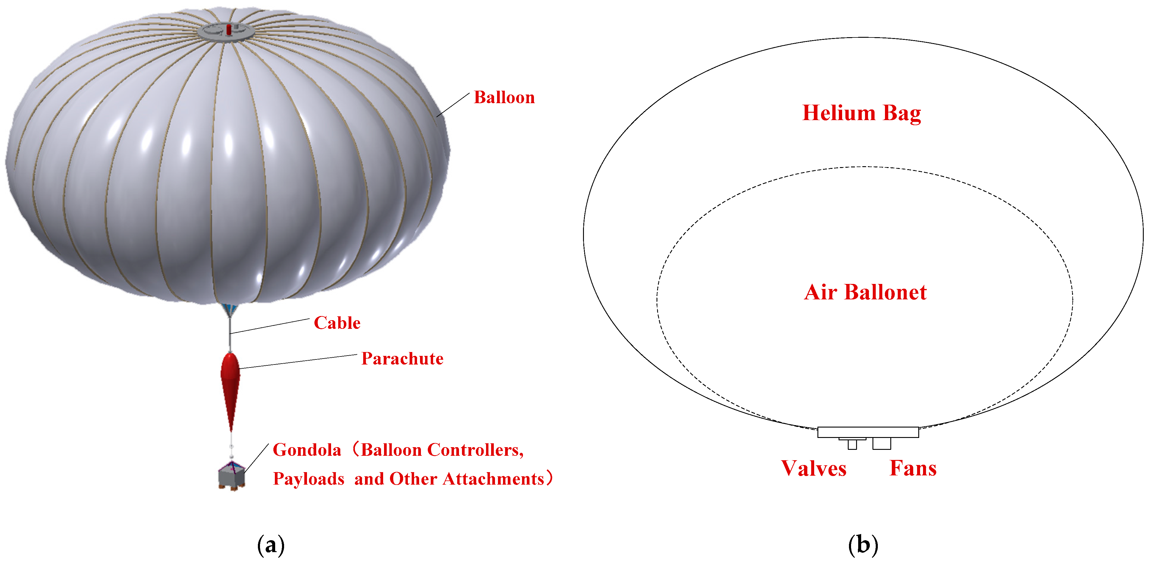
2. Overview of IPCB
3. Performance Indicator of IPCB Geometry Configuration
4. Adjustment Approaches of IPCB Geometry Configuration
- (1)
- The flight altitude of an IPB is fully controllable, and its variation depends on a rise rate and a sink rate, represented by vrise and vsink, respectively.
- (2)
- The horizontal velocity of an IPB is proportional to the local horizontal wind velocity.
- (3)
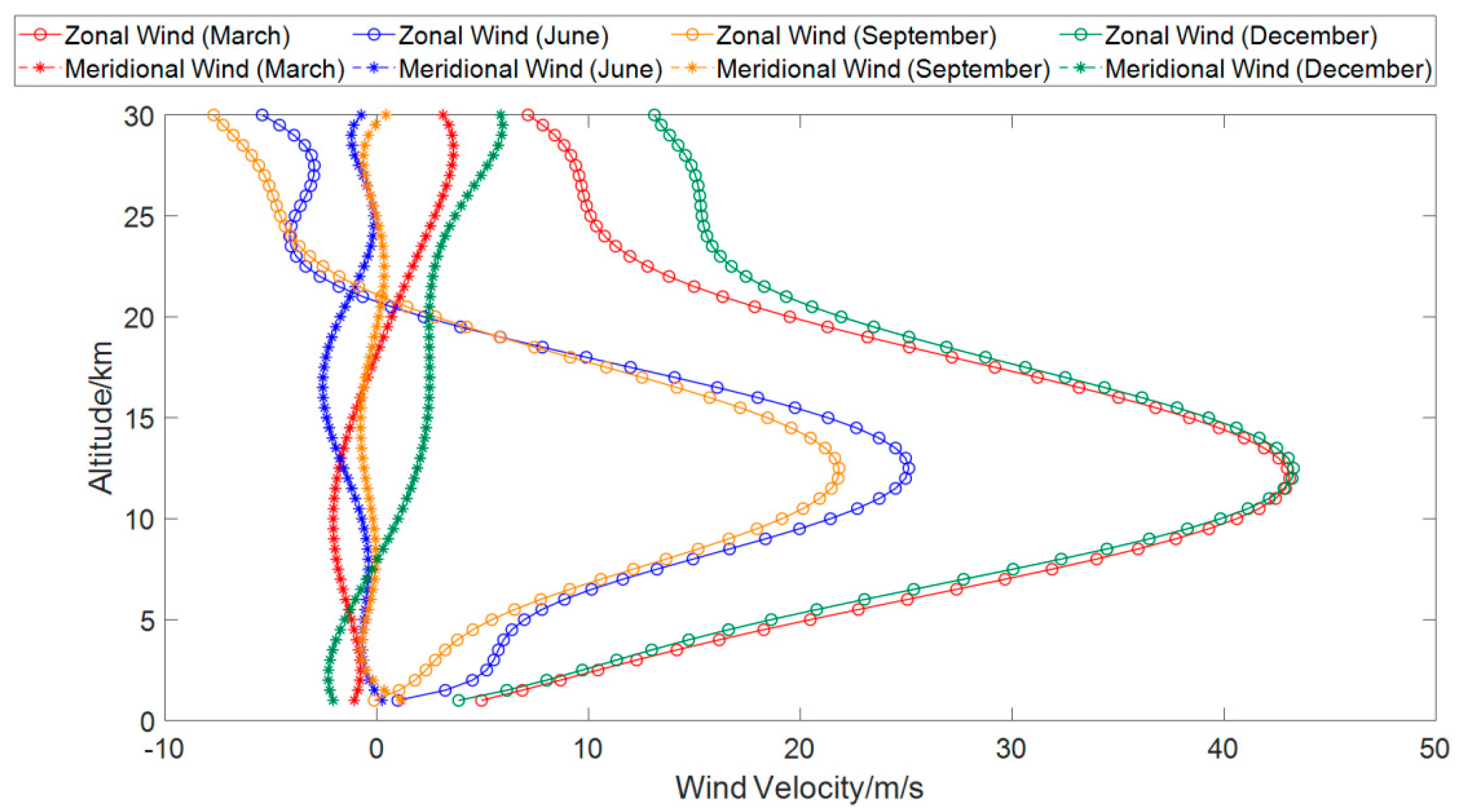
- Wind velocities vary with altitude but not with horizontal location. The wind velocities and atmosphere environment are steady during IPCB service time.
- (4)
- The influences of balloon volume variation and thermal effect on IPB motions are ignored.
4.1. Vertical Adjustment of an IPB
4.2. Horizontal Adjustment of an IPB
5. Constraints of IPCB Geometry Configuration
5.1. Airspace Constraint
5.2. Flight Altitude Constraint
5.3. Time Interval Constraint
6. Planning Algorithm of IPCB Geometry Configuration
7. Simulations and Discussions
7.1. Simulation Settings
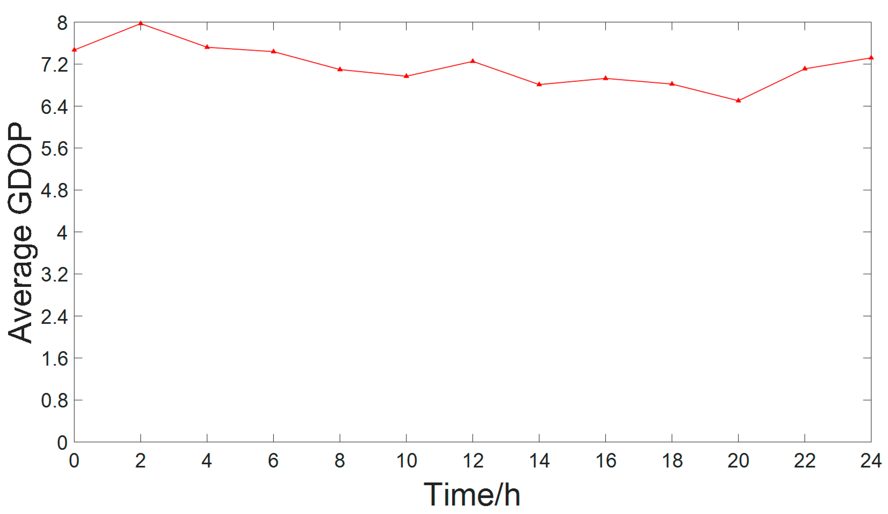
7.2. Simulation Result
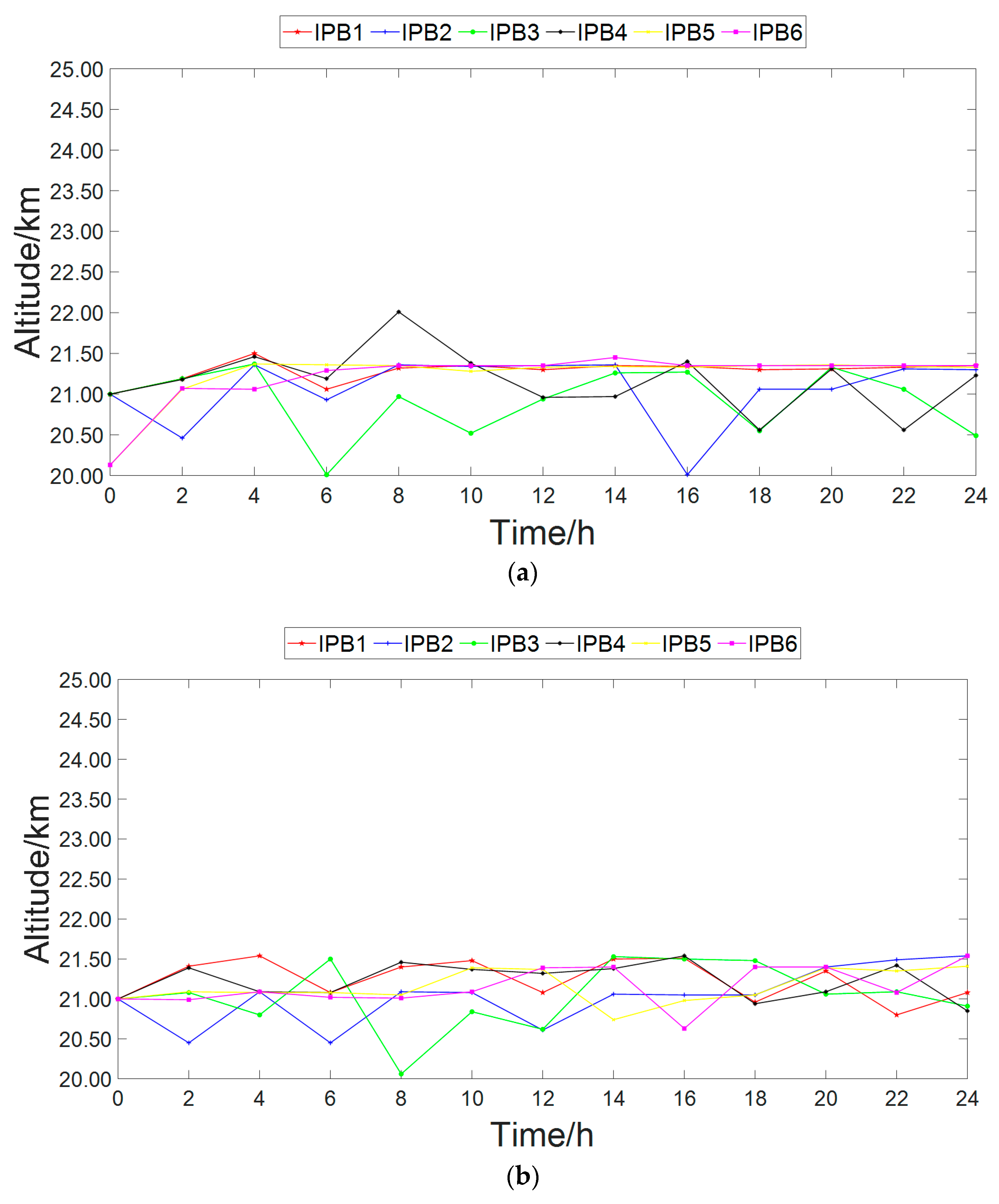
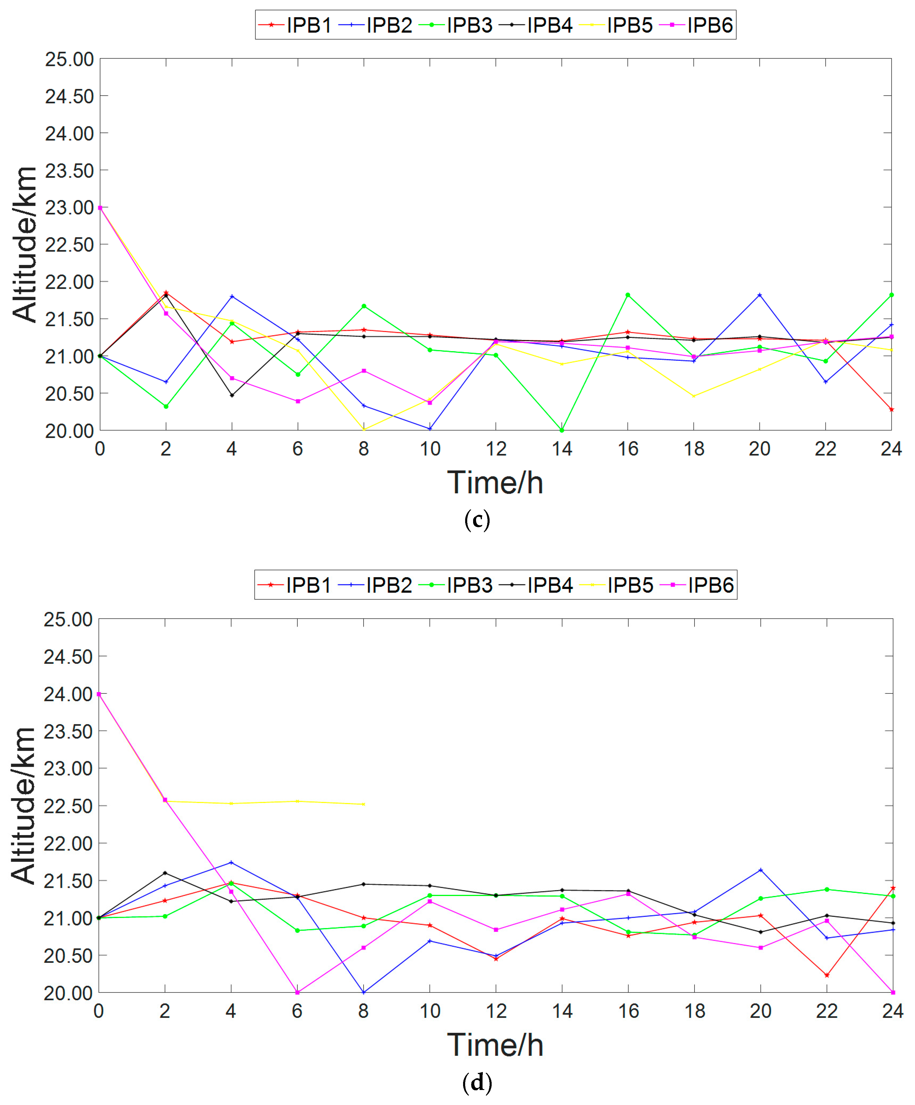
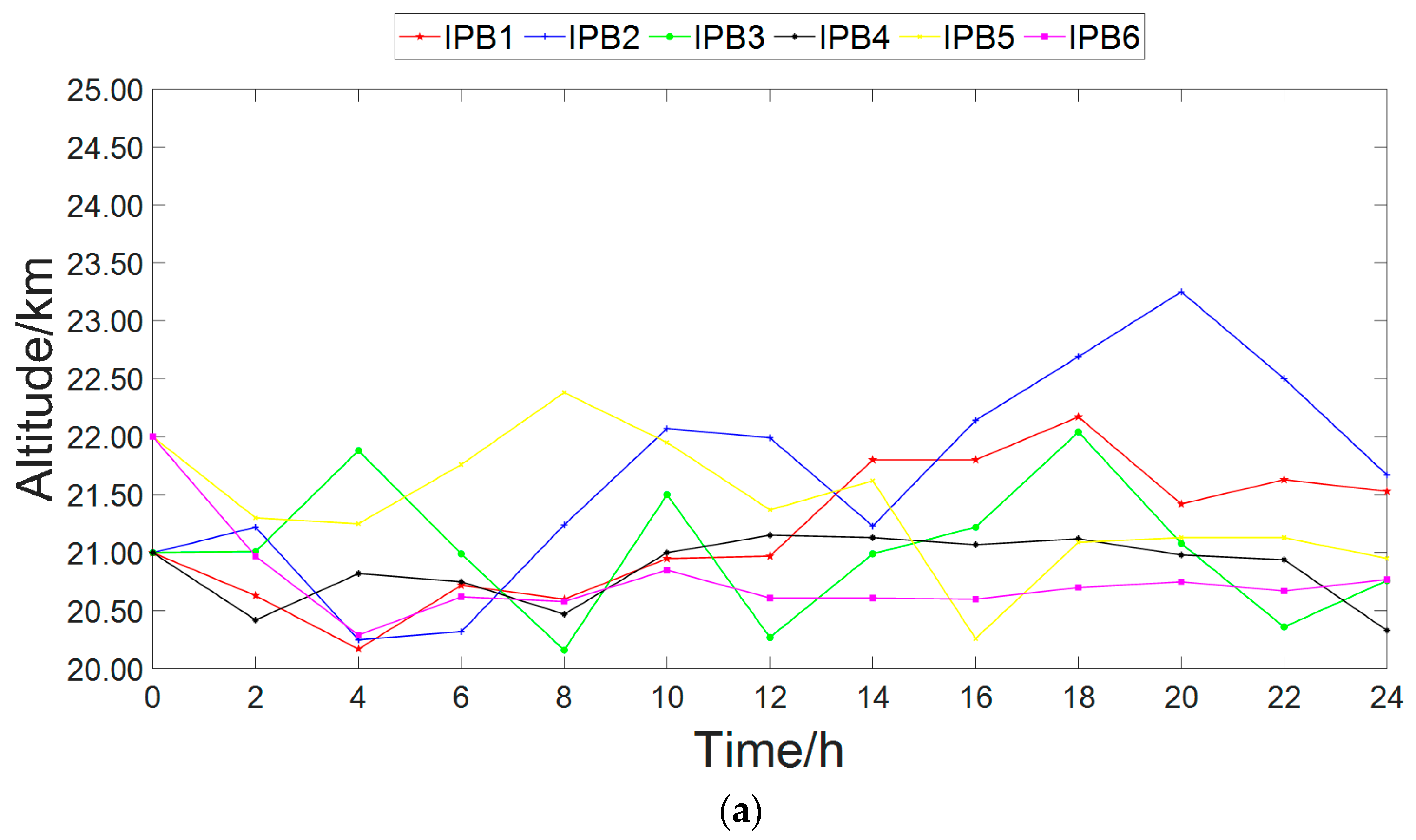
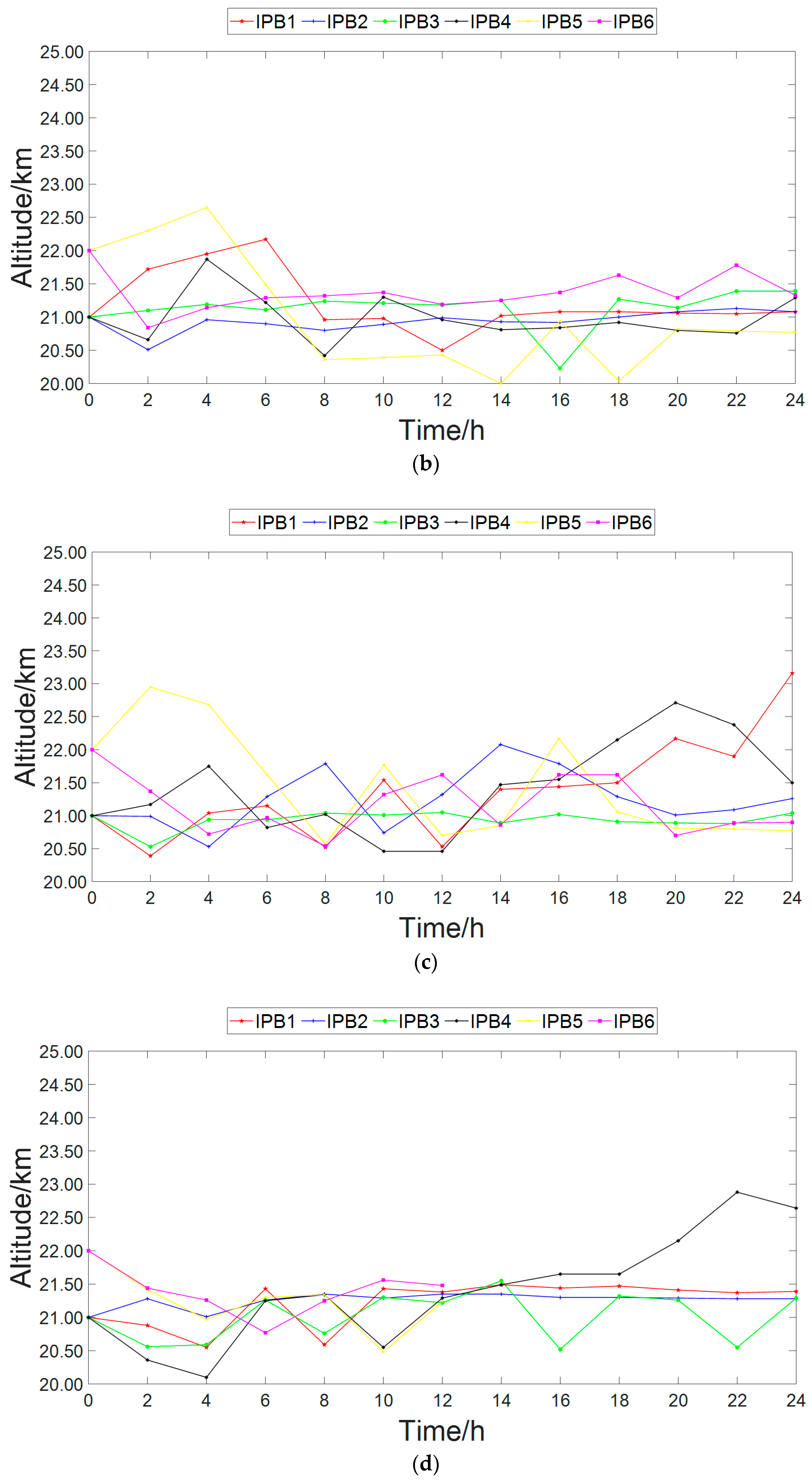
7.3. Discussion about IPCBs with Different Initial Flight Altitudes
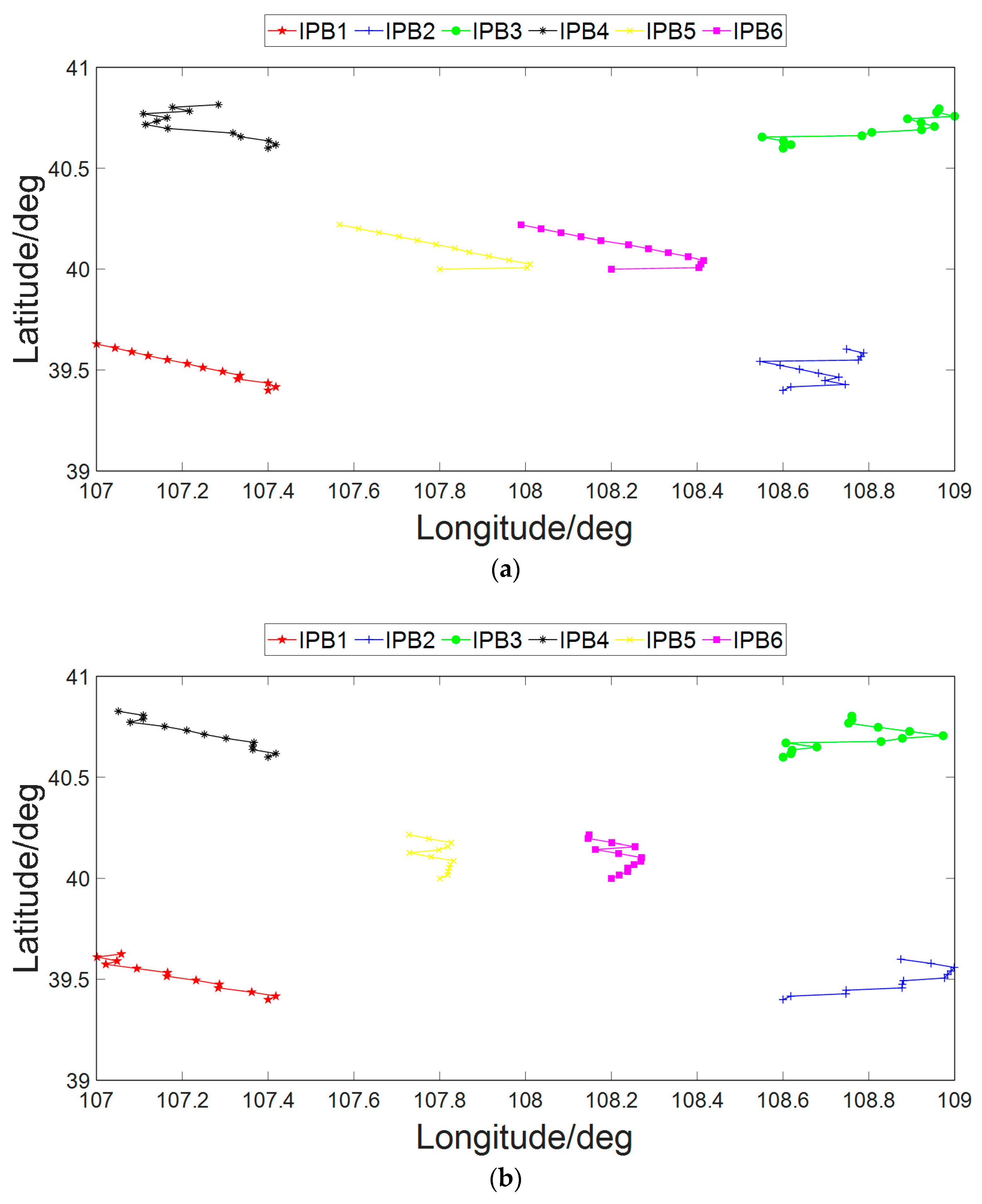
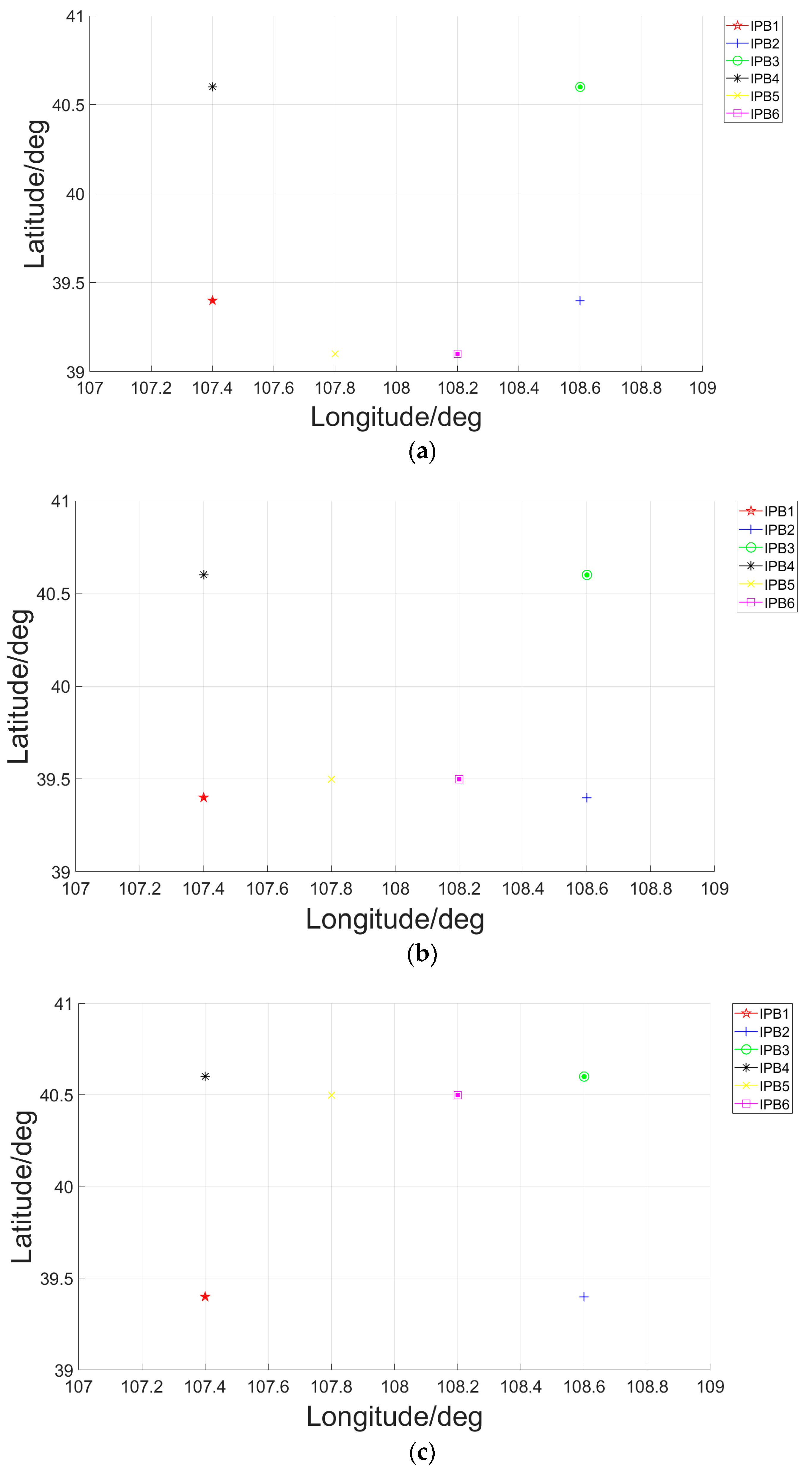
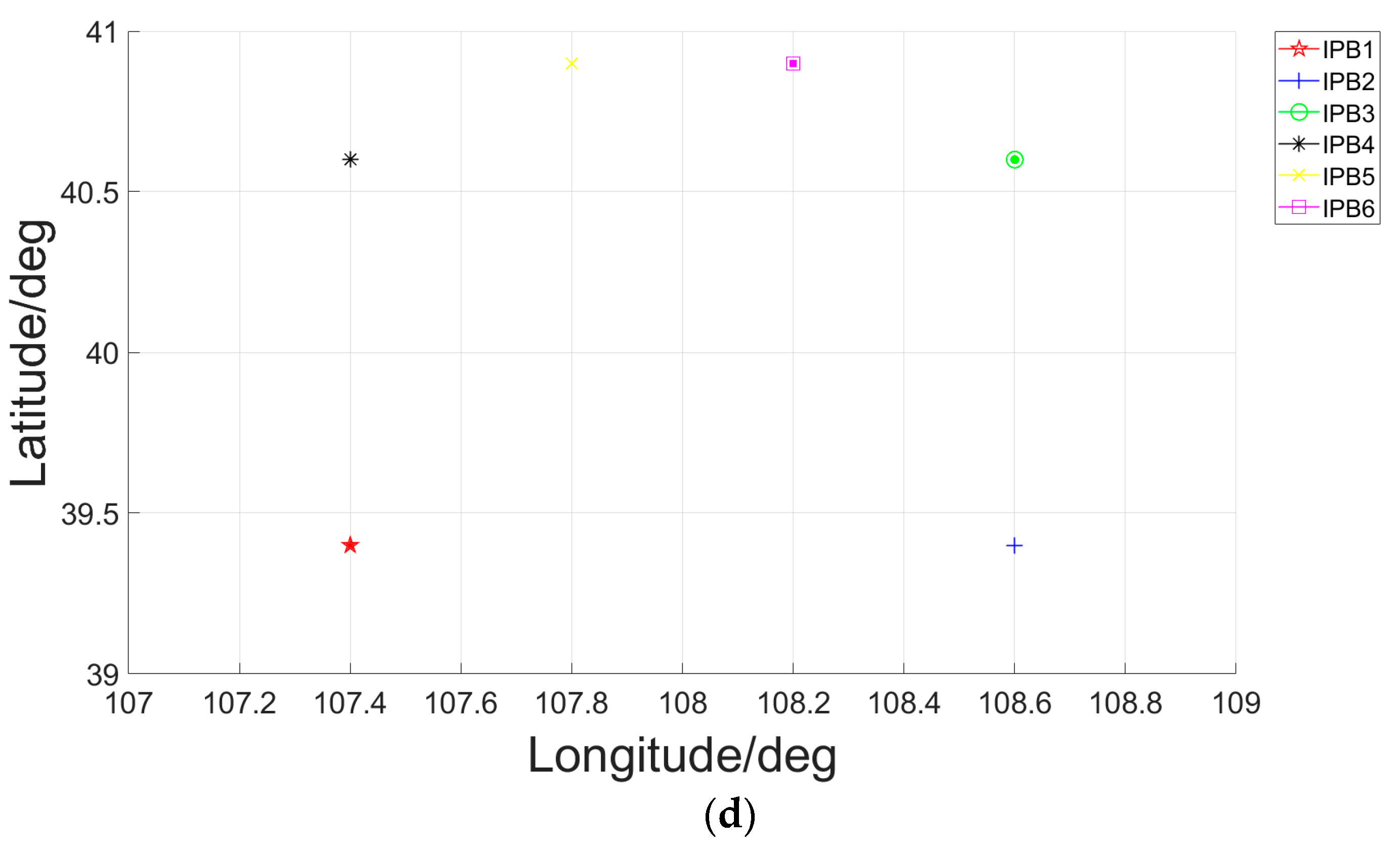
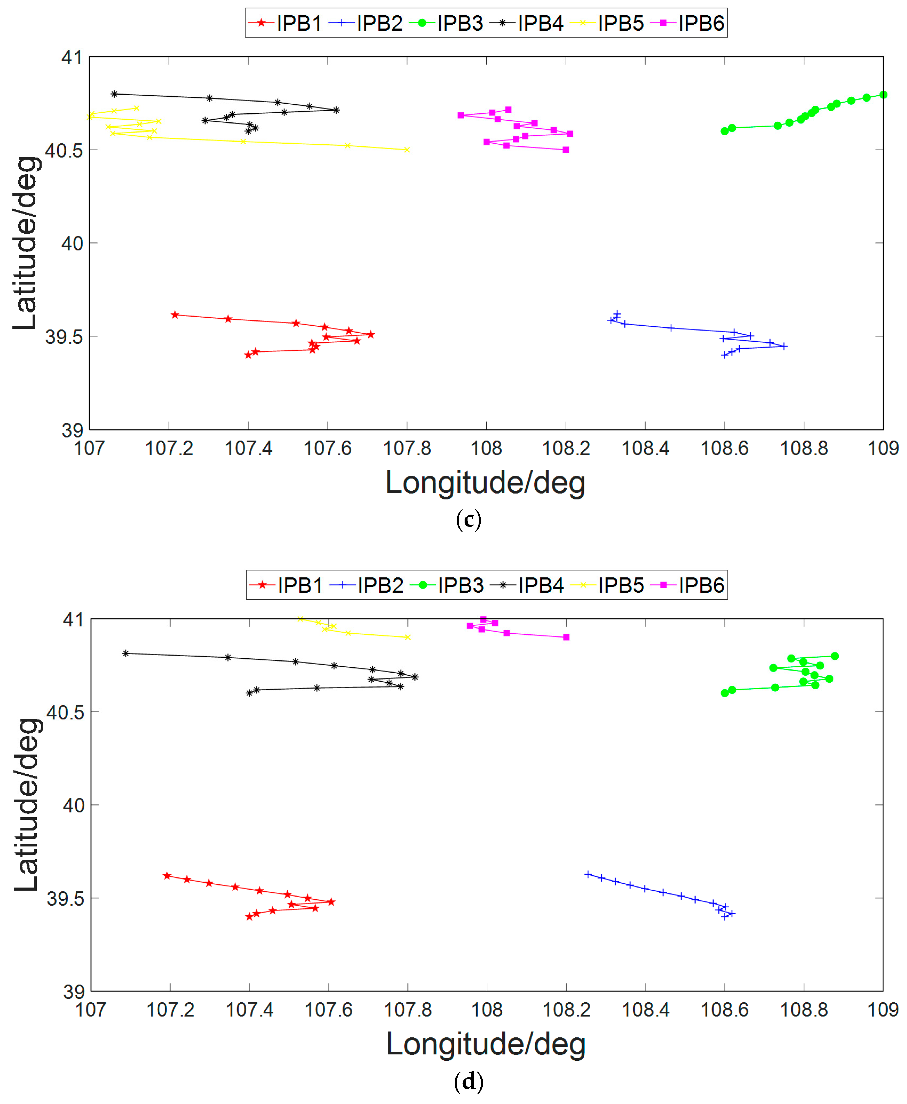
7.4. Discussion about IPCBs with Different Initial Horizontal Layouts
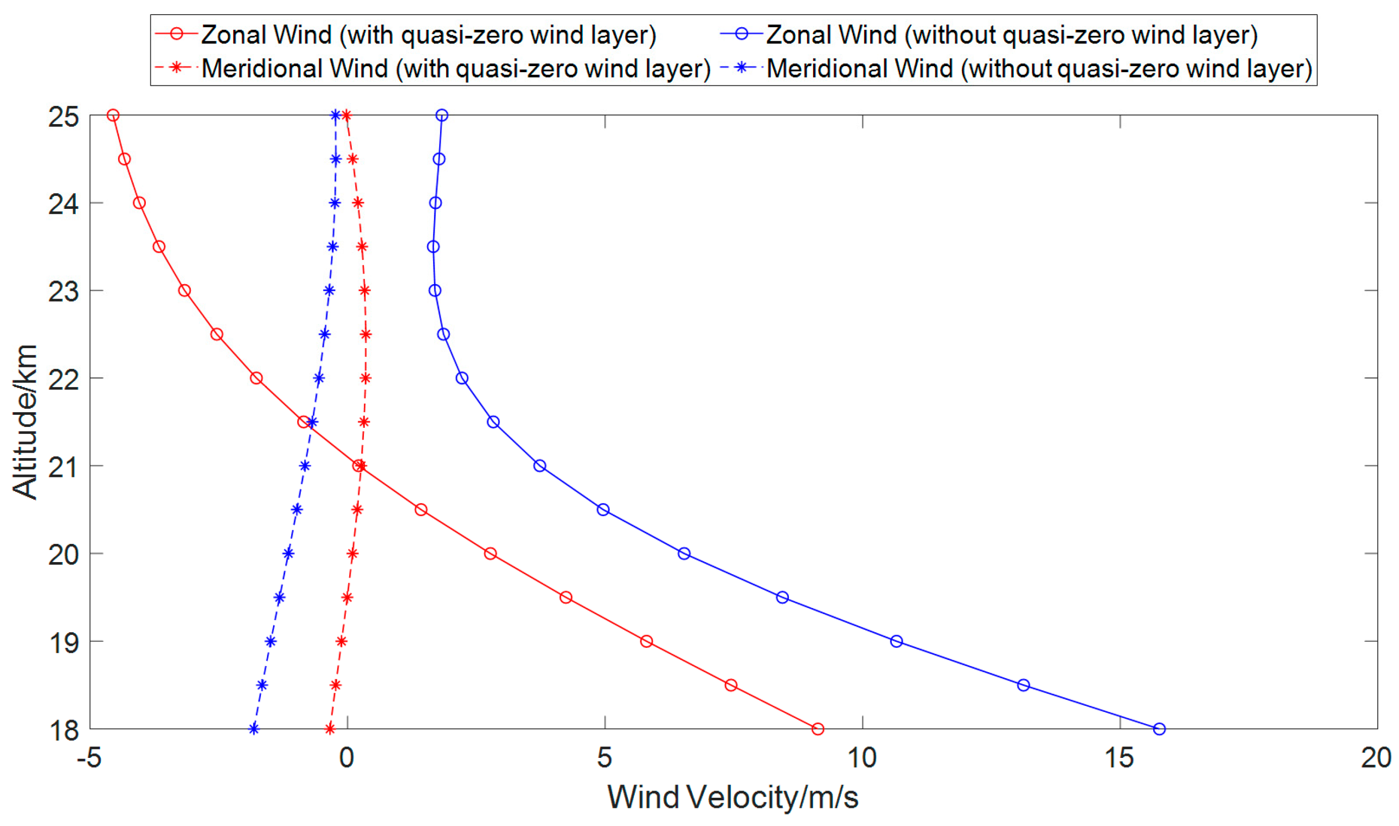
7.5. Discussion about IPCBs in Winds with/without Quasi-Zero Wind Layer
7.6. Discussion about Uncertain Environment
8. Conclusions
Author Contributions
Funding
Data Availability Statement
Conflicts of Interest
References
- Klein, D.; Parkinson, B.W. The use of pseudo-satellites for improving GPS performance. Navig. J. Inst. Navig. 1984, 31, 303–315. [Google Scholar] [CrossRef]
- Morley, T.; Lachapelle, G. GPS augmentation with pseudolites for navigation in constricted waterways. Navig. J. Inst. Navig. 1997, 44, 359–372. [Google Scholar] [CrossRef]
- Wang, J. Pseudolite applications in positioning and navigation: Progress and problems. J. Glob. Position. Syst. 2002, 1, 48–56. [Google Scholar] [CrossRef]
- Dixon, C.S.; Morrison, R.G. A pseudolite-based maritime navigation system: Concept through to demonstration. J. Glob. Position. Syst. 2008, 7, 9–17. [Google Scholar] [CrossRef]
- Ma, C.; Yang, J.; Chen, J. Satellite-Ground Joint Positioning System Based on Pseudolite. In Proceedings of the 2018 IEEE CSAA Guidance, Navigation and Control Conference, CGNCC, Xiamen, China, 10–12 August 2018. [Google Scholar] [CrossRef]
- Sheng, C.; Gan, X.; Yu, B.; Zhang, J. Precise point positioning algorithm for pseudolite combined with GNSS in a constrained observation environment. Sensors 2020, 20, 1120. [Google Scholar] [CrossRef]
- Liu, T.; Liu, J.; Wang, J.; Zhang, H.; Zhang, B.; Ma, Y.; Sun, M.; Lv, Z.; Xu, G. Pseudolites to support location services in smart cities: Review and prospects. Smart Cities 2023, 6, 2081–2105. [Google Scholar] [CrossRef]
- Kayhan, Ö.; Yücel, Ö.; Hastaoğlu, M.A. Simulation and control of serviceable stratospheric balloons traversing a region via transport phenomena and PID. Aerosp. Sci. Technol. 2016, 53, 232–240. [Google Scholar] [CrossRef]
- Jiang, Y.; Lv, M.; Zhu, W.; Du, H.; Zhang, L.; Li, J. A method of 3-D region controlling for scientific balloon long-endurance flight in the real wind. Aerosp. Sci. Technol. 2020, 97, 1–11. [Google Scholar] [CrossRef]
- Zhu, W.; Xu, Y.; Du, H.; Li, J. Thermal performance of high-altitude solar powered scientific balloon. Renew. Energy 2019, 135, 1078–1096. [Google Scholar] [CrossRef]
- Jiang, Y.; Lv, M.; Qu, Z.; Zhang, L. Performance evaluation for scientific balloon station-keeping strategies considering energy management strategy. Renew. Energy 2020, 156, 290–302. [Google Scholar] [CrossRef]
- Li, C.; Luo, R.; Chen, T. New idea for stratospheric communications—Google Loon. Commun. Technol. 2015, 48, 125–129. [Google Scholar] [CrossRef]
- Deng, X.; Yang, X.; Zhu, B.; Ma, Z.; Hou, Z. Simulation research and key technologies analysis of intelligent stratospheric aerostat Loon. Acta Aeronaut. Et Astronaut. Sin. 2023, 44, 127412. [Google Scholar] [CrossRef]
- Rabinowitz, M.; Parkinson, B.W.; Cohen, C.E.; O’Connor, M.L.; Lawrence, D.G. A system using LEO telecommunication satellites for rapid acquisition of integer cycle ambiguities. In Proceedings of the Position Location and Navigation Symposium, Palm Springs, CA, USA, 20–23 April 1996; pp. 137–145. [Google Scholar] [CrossRef]
- Li, X.; Li, X.; Ma, F.; Yuan, Y.; Zhang, K.; Zhou, F.; Zhang, X. Improved PPP ambiguity resolution with the assistance of multiple LEO constellations and signals. Remote Sens. 2019, 11, 408. [Google Scholar] [CrossRef]
- Ge, H.; Li, B.; Jia, S.; Nie, Y.; Wu, T.; Yang, Z.; Shang, J.; Zheng, Y.; Ge, M. LEO enhanced global navigation satellite system (LeGNSS): Progress, opportunities, and challenges. Geo-Spat. Inf. Sci. 2022, 25, 1–13. [Google Scholar] [CrossRef]
- Yuan, H.; Chen, X.; Luo, R.; Wan, H.; Zhang, Y.; Li, R.; Yang, G. Review of the development trend of LEO-based navigation system. Navig. Position. Timing 2022, 9, 1–11. [Google Scholar] [CrossRef]
- Zhang, Y.; Fan, L.; Liu, J.; Li, Z. Feasibility analysis of commercial broadband LEO constellation incorporated into the national comprehensive PNT system. Navig. Position. Timing 2022, 10, 26–36. [Google Scholar] [CrossRef]
- Dai, L.; Wang, J.; Tsujii, T.; Rizos, C. Pseudolite Applications in Positioning and Navigation: Modelling and Geometric Analysis. In Proceedings of the International Symposium on Kinematic Systems in Geodesy, Geomatics & Navigation (KIS2001), Banff, AB, Canada, 5–8 June 2001. [Google Scholar]
- Chandu, B.; Pant, R.S.; Moudgalya, K. Modeling and Simulation of a Precision Navigation System Using Pseudolites Mounted on Airships. In Proceedings of the 7th AIAA Aviation Technology, Integration and Operations Conference, Belfast, Northern Ireland, 18–20 September 2007. [Google Scholar]
- Oktay, H. Airborne pseudolites in a global positioning system degraded environment. In Proceedings of the 5th International Conference on Recent Advances in Space Technologies–RAST2011, Istanbul, Turkey, 9–11 June 2011. [Google Scholar] [CrossRef]
- Tsujii, T.; Harigae, M.; Barnes, J.; Wang, J.; Rizos, C. Experiments of inverted pseudolite positioning for airship-based GPS augmentation system. In Proceedings of the 15th International Technical Meeting of the Satellite Division of the U.S. Institute of Navigation, Portland, OR, USA, 24–27 September 2002; pp. 1689–1695. [Google Scholar]
- Sultana, Q.; Sunehra, D.; Ratnam, D.V.; Rao, P.S.; Sarma, A.D. Significance of instrumental biases and dilution of precision in the context of GAGAN. Indian J. Radio Space Phys. 2007, 36, 405–410. [Google Scholar]
- Quddusa, S.; Dhiraj, S.; Vemuri, S.S.; Achanta, D.S. Effects of pseudolite positioning on DOP in LAAS. Positioning 2010, 1, 18–26. [Google Scholar] [CrossRef]
- Wang, J.; Li, H.; Lu, J.; Li, K.; Li, H.; Yang, L.; Li, Y. A PSO-Based Layout Method for GNSS Pseudolite System. In Proceedings of the ICIT 2017, Singapore, 27–29 December 2017. [Google Scholar] [CrossRef]
- Jiang, M.; Li, R.; Liu, W. Research on geometric configuration of pseudolite positioning system. Comput. Eng. Appl. 2017, 53, 271–276. [Google Scholar]
- Tang, W.; Chen, J.; Yu, C.; Ding, J.; Wang, R. A new ground-based pseudolite system deployment algorithm based on MOPSO. Sensors 2021, 21, 5364. [Google Scholar] [CrossRef]
- Du, H.; Lv, M.; Li, J.; Zhu, W.; Zhang, L.; Wu, Y. Station-keeping performance analysis for high altitude balloon with altitude control system. Aerosp. Sci. Technol. 2019, 92, 644–652. [Google Scholar] [CrossRef]
- Du, H.; Li, J.; Zhu, W.; Qu, Z.; Zhang, L.; Lv, M. Flight performance simulation and station-keeping endurance analysis for stratospheric super-pressure balloon in real wind field. Aerosp. Sci. Technol. 2019, 86, 1–10. [Google Scholar] [CrossRef]
- Du, H.; Lv, M.; Zhang, L.; Zhu, W.; Wu, Y.; Li, J. Energy management strategy design and station-keeping strategy optimization for high altitude balloon with altitude control system. Aerosp. Sci. Technol. 2019, 93, 1–9. [Google Scholar] [CrossRef]
- Song, J.; Hou, C.; Xue, G.; Ma, M. Study of constellation design of pseudolites based on improved adaptive genetic algorithm. J. Commun. 2016, 11, 879–885. [Google Scholar] [CrossRef]
- Tian, R.; Cui, Z.; Zhang, S.; Wang, D. Overview of navigation augmentation technology based on LEO. Navig. Position. Timing 2021, 8, 66–81. [Google Scholar] [CrossRef]
- Kaplan, E.D.; Hegarty, C.J. Understanding GPS: Principles and Applications, 2nd ed; Artech House Inc.: Norword, MA, USA, 2006; p. 02062. [Google Scholar]
- Teng, Y.; Wang, J.; Huang, Q. Mathematical minimum of geometric dilution of precision (GDOP) for dual-GNSS constellations. Adv. Space Res. 2016, 57, 183–188. [Google Scholar] [CrossRef]
- Nalineekumari, A.; Sasibhushana, R.G.; Ashok, K.N. GDOP analysis with optimal satellite using GA for southern region of Indian subcontinent. Procedia Comput. Sci. 2018, 143, 303–308. [Google Scholar] [CrossRef]
- Teng, Y.; Wang, J. A closed-form formula to calculate geometric dilution of precision (GDOP) for multi-GNSS constellations. GPS Solut. 2016, 20, 331–339. [Google Scholar] [CrossRef]
- Li, D.; Deng, P.; Liu, B.; Qu, Y.; Zeng, L.; Liu, T. Research on the Dynamic Configuration of Air-Based Pseudolite Network. In China Satellite Navigation Conference (CSNC) 2015 Proceedings; Springer: Berlin/Heidelberg, Germany, 2015; Volume II, pp. 357–367. [Google Scholar]
- Blackmore, B.; Kuwata, Y.; Wolf, M.T.; Assad, C.; Fathpour, N.; Newman, C.; Elfes, A. Global Reachability and Path Planning for Planetary Exploration with Montgolfirer Balloons. In Proceedings of the 2010 IEEE International Conference on Robotics and Automation, Anchorage Convention District, Anchorage, AK, USA, 3–8 May 2010. [Google Scholar]
- Wolf, M.T.; Blackmore, L.; Kuwata, Y.; Fathpour, N.; Newman, C. Probabilistic Motion Planning of Balloons in Strong, Uncertain Wind Fields. In Proceedings of the IEEE International Conference on Robotics & Automation, Anchorage, AK, USA, 3–7 May 2010. [Google Scholar] [CrossRef]
- Zhai, J.; Yang, X.; Deng, X.; Long, Y.; Zhang, J.; Bai, F. Global path planning of stratospheric aerostat in uncertain wind field. J. Beijing Univ. Aeronaut. Astronaut. 2023, 49, 1116–1126. [Google Scholar] [CrossRef]
- Bellemare, M.G.; Candido, S.; Castro, P.S.; Gong, J.; Machado, M.C.; Moitra, S.; Ponda, S.S.; Wang, Z. Autonomous navigation of stratospheric balloons using reinforcement learning. Nature 2020, 588, 77–82. [Google Scholar] [CrossRef]
- Furfaro, R.; Lunine, J.I.; Elfes, A.; Reh, K. Wind-based navigation of a hot-air balloon on Titan: A feasible study. In Proceedings of the SPIE Defense and Security Symposium, Orlando, FL, USA, 18–20 March 2008. [Google Scholar] [CrossRef]
- Hedin, A.E.; Biondi, M.A.; Burnside, R.G.; Hernandez, G.; Johnson, R.M.; Killeen, T.L.; Mazaudier, C.; Meriwether, J.W.; Salah, J.E.; Sica, R.J.; et al. Revised global model of thermosphere winds using satellite and ground-based observations. J. Geophys. Res. 1991, 96, 7657–7688. [Google Scholar] [CrossRef]
- Mueller, J.B.; Zhao, Y.J.; Garrard, W.L. Optimal ascent trajectories for stratospheric airships using wind energy. J. Guid. Control. Dyn. 2009, 32, 1232–1245. [Google Scholar] [CrossRef]
- Lee, S.; Bang, H. Three-dimensional ascent trajectory optimization for stratospheric airship platforms in the jet stream. J. Guid. Control. Dyn. 2007, 30, 1341–1352. [Google Scholar] [CrossRef]
- Sun, S.; Li, Z.; Tian, K. Modeling and trajectory planning of return process for a class of airship with wind field. Aerosp. Control. Appl. 2014, 40, 37–41. [Google Scholar] [CrossRef]
- Zhang, X.; Chen, L.; Quan, T. Study of ascent trajectory for stratospheric airship in the jet stream. Electron. Des. Eng. 2014, 22, 11–13. [Google Scholar]
- Belmont, A.D.; Dartt, D.G.; Nastrom, G.D. Variations of stratospheric zonal winds, 20–65 km, 1961–1971. J. Appl. Meteorol. 1975, 14, 585–594. [Google Scholar] [CrossRef]
- Tao, M.; He, J.; Liu, Y. Analysis of the characteristics of the stratospheric quasi-zero wind layer and the effects of the quasi-biennial oscillation on it. Clim. Environ. Res. 2012, 17, 92–102. [Google Scholar] [CrossRef]
- Chang, X.; Bai, Y.; Fu, W.; Yan, J. Research on fixed-point aerostat based on its special stratosphere wind field. J. Northwestern Polytech. Univ. 2014, 32, 12–17. [Google Scholar]
- Deng, X.; Li, K.; Yu, C.; Yang, X.; Hou, Z. Station-keeping performance of novel near-space aerostat in quasi-zero wind layer. J. Natl. Univ. Def. Technol. 2019, 41, 5–12. [Google Scholar] [CrossRef]
- Chen, B.; Liu, Y.; Liu, L.; Shen, X.; Zhang, Y. Characteristics of spatial–temporal distribution of the stratospheric quasi-zero wind layer in low-latitude regions. Clim. Environ. Res. 2018, 23, 657–669. [Google Scholar] [CrossRef]
- Roney, J.A. Statistical wind analysis for near-space applications. J. Atmos. Sol. Terr. Phys. 2007, 69, 1485–1501. [Google Scholar] [CrossRef]
- Mirjalili, S.; Lewis, A. The whale optimization algorithm. Adv. Eng. Softw. 2016, 95, 51–67. [Google Scholar] [CrossRef]
- Mafarja, M.M.; Mirjalili, S. Hybrid whale optimization algorithm with simulated annealing for feature selection. Neurocomputing 2017, 260, 302–312. [Google Scholar] [CrossRef]
- Xiong, G.; Zhang, J.; Shi, D.; He, Y. Parameter extraction of solar photovoltaic models using an improved whale optimization algorithm. Energy Convers. Manag. 2018, 174, 388–405. [Google Scholar] [CrossRef]
- Ling, Y.; Zhou, Y.; Luo, Q. Lévy flight trajectory-based whale optimization algorithm for global optimization. IEEE Access 2017, 5, 6168–6186. [Google Scholar] [CrossRef]
- Yan, Z.; Wang, S.; Liu, B.; Li, X. Application of Whale Optimization Algorithm in Optimal Allocation of Water Resources. In Proceedings of the 2018 3rd International Conference on Advances in Energy and Environment Research (ICAEER 2018), Guilin, China, 10–12 August 2018. [Google Scholar] [CrossRef]
- Kennedy, J.; Eberhart, R. Particle Swarm Optimization. In Proceedings of the ICNN95–International Conference on Neural Networks, Perth, WA, Australia, 27 November–1 December 1995. [Google Scholar] [CrossRef]
- Neri, R.; Tirronen, V. Scale factor local search in differential evolution. Memetic Comp. 2009, 1, 153–171. [Google Scholar] [CrossRef]
- Conway, J.P.; Bodeker, G.E.; Waugh, D.W.; Murphy, D.J.; Cameron, C.; Lewis, J. Using project Loon superpressure balloon observations to investigate the inertial peak in the intrinsic wind spectrum in the midlattitude stratosphere. J. Geophys. Res. Atmos. 2019, 124, 8594–8604. [Google Scholar] [CrossRef]


| Symbol | Physical Meaning | Value |
|---|---|---|
| np | number of IPBs in a constellation initially | 6 |
| nt | expected service duration of an IPCB | 24 h |
| cm | meridional wind coefficients | −0.1338, 1.3189, −1.9669, −2.3772, 4.0187, 1.4032, −1.4290, −0.5504 |
| cz | zonal wind coefficients | 2.1927, −7.6660, −3.0280,28.8161, −2.6879, −41.5979, 2.0248, 21.8084 |
| λmin | minimal longitude of the approved airspace | 107° E |
| λmax | maximal longitude of the approved airspace | 109° E |
| ϕmin | minimal latitude of the approved airspace | 39° N |
| ϕmax | maximal latitude of the approved airspace | 41° N |
| hmin | feasible minimal flight altitude of an IPB | 20 km |
| hmax | feasible maximal flight altitude of an IPB | 24 km |
| IPB | Longitude | Latitude | Flight Altitude |
|---|---|---|---|
| IPB 1 | 107.4° E | 39.4° N | 21 km |
| IPB 2 | 108.6° E | 39.4° N | 21 km |
| IPB 3 | 108.6° E | 40.6° N | 21 km |
| IPB 4 | 107.4° E | 40.6° N | 21 km |
| IPB 5 | 107.8° E | 40° N | 22 km |
| IPB 6 | 108.2° E | 40° N | 22 km |
| Initial Flight Altitude of IPB5 and IPB6/km | Average GDOP |
|---|---|
| 20 | 7.26 |
| 21 | 7.14 |
| 22 | 7.32 |
| 23 | 7.47 |
| 24 | 8.64 |
| Initial Horizontal Layout | Average GDOP |
|---|---|
| Layout 1 | 10.88 |
| Layout 2 | 9.53 |
| Layout 3 | 7.32 |
| Layout 4 | 10.83 |
| Layout 5 | 22.14 |
| Symbol | Physical Meaning | Value |
|---|---|---|
| cm | meridional wind coefficients | −0.5066, 4.3171, −14.6477, 27.7923, −36.4969, 32.8921, −13.9287, −0.2023 |
| cz | zonal wind coefficients | −40.2337, 321.8428, −1018.3275, 1597.1910, −1263.8719, 461.2160, −94.6881, 40.2845 |
Disclaimer/Publisher’s Note: The statements, opinions and data contained in all publications are solely those of the individual author(s) and contributor(s) and not of MDPI and/or the editor(s). MDPI and/or the editor(s) disclaim responsibility for any injury to people or property resulting from any ideas, methods, instructions or products referred to in the content. |
© 2024 by the authors. Licensee MDPI, Basel, Switzerland. This article is an open access article distributed under the terms and conditions of the Creative Commons Attribution (CC BY) license (https://creativecommons.org/licenses/by/4.0/).
Share and Cite
Qu, Y.; Wang, S.; Pan, T.; Feng, H. IPCB: Intelligent Pseudolite Constellation Based on High-Altitude Balloons. Electronics 2024, 13, 2095. https://doi.org/10.3390/electronics13112095
Qu Y, Wang S, Pan T, Feng H. IPCB: Intelligent Pseudolite Constellation Based on High-Altitude Balloons. Electronics. 2024; 13(11):2095. https://doi.org/10.3390/electronics13112095
Chicago/Turabian StyleQu, Yi, Sheng Wang, Tianshi Pan, and Hui Feng. 2024. "IPCB: Intelligent Pseudolite Constellation Based on High-Altitude Balloons" Electronics 13, no. 11: 2095. https://doi.org/10.3390/electronics13112095
APA StyleQu, Y., Wang, S., Pan, T., & Feng, H. (2024). IPCB: Intelligent Pseudolite Constellation Based on High-Altitude Balloons. Electronics, 13(11), 2095. https://doi.org/10.3390/electronics13112095