Multitask Learning for Concurrent Grading Diagnosis and Semi-Supervised Segmentation of Honeycomb Lung in CT Images

Abstract

Honeycomb lung is a radiological manifestation of various lung diseases, seriously threatening patients’ lives worldwide. In clinical practice, the precise localization of lesions and assessment of their severity are crucial. However, accurate segmentation and grading are challenging for physicians due to the heavy annotation burden and diversity of honeycomb lungs. In this paper, we propose a multitask learning architecture for semi-supervised segmentation and grading diagnosis to achieve automatic localization and assessment of lesions. To the best of our knowledge, this is the first method that integrates a grading diagnosis task into honeycomb lung semi-supervised segmentation. Firstly, we adapt cross-learning to capture local features and long-range dependencies from the CNN and transformer. Secondly, considering the diversity of honeycomb lung lesions, the shape-edge aware constraint is designed to assist the model in locating lesions. Then, in order to better understand the different levels of information in the images, we develop global contrast and local contrast learning to enhance the model’s learning of semantic-level and pixel-level features. Lastly, aiming to improve the diagnostic accuracy, we propose a gradient thresholding algorithm to integrate the segmentation predictions into the grading diagnosis network. The experiment’s results based on the in-house honeycomb lung dataset demonstrate the superiority of our method. Compared to other methods, our approach achieves a state-of-the-art performance. In particular, in external data testing, our predictions are consistent with physicians in the majority of cases. In addition, the segmentation results based on the public Kvasir-SEG dataset also indicate that our method has good generalization ability.

1. Introduction

Honeycomb lung is a clinical manifestation of various lung diseases [1,2,3] which pose a significant threat to patients [4,5,6]. It is important to accurately assess the severity of honeycomb lung to assist physicians in diagnosing and making follow-up treatment plans [7]. Honeycomb lung patients face different treatment options at different grades [8]. For early-stage patients, antacid medication is mainly used to improve respiratory outcomes [9]. For patients in the middle and late stages, respiratory support or oxygen therapy is usually used to prolong life [10,11]. Therefore, rapid and accurate judgment of disease staging is essential to help prolong patient survival and alleviate suffering [12].

In clinical diagnosis, computed tomography (CT) is a key and intuitive tool for quantifying and grading diseases [13,14]. On the basis of factors such as the texture, location, and size of the diseased tissue, honeycomb lung can be classified into four grades, as shown in Figure 1: early stage (I), progressive stage (II), intermediate and late stage (III), and terminal stage (IV). The red box and green outlined areas indicate honeycomb lesions.However, reading an image with several slices to accurately grade disease is time-consuming and laborious. In addition, the confusion surrounding honeycomb lungs, as well as their diversity, between different grades makes the manual annotation of lesions more challenging. To alleviate the workload and improve the diagnostic efficiency of doctors, automatic classification and segmentation of honeycomb lungs is highly demanded. Classification tasks typically depend on the feature extraction capabilities of a convolutional neural network (CNN) to distinguish lesion images [15,16]. For segmentation tasks, U-Net and its variants are usually used to perform pixel-level classification of diseased tissue [17,18]. Notably, most studies have only conducted classification and segmentation tasks separately, while the two tasks can be connected to construct a joint network for classification and segmentation to improve the overall performance.

Previous studies have demonstrated the superiority of some models in the task of lesion segmentation, but they rely highly on the pixel-level annotation of large-scale datasets [19]. In general, pixel-by-pixel annotation of images is laborious and time-consuming, which is difficult for doctors with heavy workloads. Recently, many semi-supervised segmentation methods [20] have been developed to address the annotation problem by leveraging limited annotated data and a large amount of unannotated data. The mainstream semi-supervised deep learning methods include pseudo-labeling [21], entropy minimization [22], and consistency regularization [23]. The above methods have achieved promising results by perturbing image data or constraining models to obtain a robust network. However, these methods ignore the context-rich latent features at different representation levels which limits the performance of the model. On the other hand, they do not take into account the shape information of the target area, resulting in insufficient awareness of boundaries.

Considering the above problems, contrastive learning has been introduced into semi-supervised segmentation tasks in recent years [24]. For image-level contrastive algorithms [25], similar images are regarded as positive sample pairs, while dissimilar images are regarded as negative sample pairs. For pixel-level contrastive algorithms [26], the positive sample pairs consist of pixels at the same position in the images, while the negative sample pairs consist of pixels at different positions. During training, similar sample pairs are encouraged to pull each other, while dissimilar sample pairs are encouraged to push each other, eventually achieving the purpose of capturing the inherent feature representation of the target areas. In addition, some works [27,28] attempt to impose explicit shape constraints or add input image shape information to enhance the boundary segmentation capabilities of the model. Nevertheless, most previous studies have not simultaneously considered multilevel contrast learning between features of different paradigms and shape-edge constraints of input features, resulting in insufficient segmentation of complex edge and fuzzy regions.

On the other hand, in disease-grading diagnosis, some studies [29,30,31] have taken into account the use of deep learning methods based on imaging data. These methods generally use a CNN to extract features from different levels of lesion images to achieve the automatic grading of specific diseases. However, few methods have been designed to combine grading diagnosis with semi-supervised segmentation to boost overall performance. In fact, grading diagnosis can help the segmentation network distinguish lesion areas. Meanwhile, the segmentation network also provides lesion location and size information to the classification network. Therefore, we believe that it is beneficial to combine the two tasks for the classification and segmentation of honeycomb lung CT images.

In this paper, based on the above analysis, we propose a multitask learning model that consists of disease-grading diagnosis and semi-supervised segmentation. Specifically, the semi-supervised segmentation network is composed of a CNN and a transformer, and it learns high-confidence labels under different paradigms through cross-supervision. Then, global and local contrastive learning strategies are developed to extract potential feature representations at different levels. Lastly, considering the complex contours of the lesion regions, we design a novel shape-edge aware constraint. On the other hand, for the classification network, a disease assessment network is constructed based on a CNN. In particular, we propose a gradient thresholding algorithm that provides information about the size of the lesions to assist the grading network to learn different grades of lesion images. Compared to previous work, our contributions can be summarized as follows:

(1)

We propose a multitask model that combines disease assessment and semi-supervised segmentation for grading and segmenting honeycomb lung CT images. To the best of our knowledge, this is the first method to simultaneously grade and segment honeycomb lung CT images.

(2)

In order to utilize the lesion area information provided by the segmentation network, a gradient thresholding algorithm is developed and integrated into the grading network to assist in distinguishing different levels of images.

(3)

Considering the complex contours of the lesion area, we design a novel shape-edge constraint strategy to improve the boundary awareness of the segmentation network.

(4)

To alleviate the annotation burden, we design a semi-supervised network consisting of a CNN and transformer to segment the lesion areas. In addition, to improve segmentation performance, global and local contrastive learning methods are adopted to learn inherent features at different levels.

(5)

The results of the experiment demonstrate the superiority of our model’s segmentation using in-house honeycomb lung and public Kavsir-SEG datasets. Furthermore, our grading network also achieved promising results that are consistent with expert physician evaluations.

(6)

Following the principles of data sharing and community advancement, our honeycomb dataset is available at https://github.com/YangBingQ/MTGS and was accessed on 27 May 2024.

2. Related Work

2.1. Semi-Supervised Segmentation

Because of limited amount of annotated data, many studies focus on semi-supervised learning, which utilizes a few annotated data points and a large amount of unlabeled data to achieve satisfactory results and alleviate annotation costs. The current dominant semi-supervised segmentation methods can be divided into several categories. The first category is pseudo-labeling, which aims to assign labels to unlabeled images iteratively. The pseudo-labels are then used together with labeled images for training. For example, Lu et al. [32] used an uncertainty-aware approach to generate more stable and reliable pseudo-labels and then iteratively trained the network with annotated images. The second category of methods is entropy minimization, which requires the model to produce low-entropy predictions on unlabeled data and avoid class overlap. MixMatch [33] is a classical entropy minimization method that designed a sharpening function to guess unlabeled data with minimum entropy. The other method involves adversarial networks to pull the distributions of unlabeled and labeled data. Commonly used adversarial networks include variational autoencoder (VAE) [34], generative adversarial network (GAN) [35], and graph convolutional networks (GCNs) [36]. Lastly, consistency regularization is a popular method that is widely used in semi-supervised learning [23]. In detail, it can be classified into network-level consistency and task-level consistency. For instance, Wang et al. [24] introduced a reconstruction task and a signed distance field (SDF) prediction task to capture semantic information and shape constraints, respectively, further improving segmentation performance. Luo et al. [37] explored the feature complementarity of unlabeled data between different network paradigms of a CNN and transformer. Notably, contrastive learning has received a lot of interest and has been applied to many semi-supervised segmentation methods. Generally, pixel-level contrast learning helps the network extract more spatial information from an image [38]. However, most work has only adopted single-level contrastive learning and does not consider multilevel feature representations. Additionally, few studies have focused on shape-edge constraints for complex lesions. In this work, we mainly concentrate on semi-supervised segmentation methods with shape-edge awareness and multilevel contrastive learning under different network paradigms.

2.2. Grading Diagnosis

The accurate identification and grading of disease severity is important in clinical diagnosis. The automated classification algorithm can provide doctors with intelligent assistance and improve diagnosis and treatment efficiency. Recently, many deep learning methods have been designed for various disease classifications. Generally, most methods use convolutional neural networks. For example, Abramovich et al. [39] proposed the Fundus-Net model to grade the severity of lesions in fundus images on a range of 1 to 10 and achieved satisfactory results. A deep neural network was developed [40] to classify sagittal lumbar spine MRI images based on the severity of intervertebral disc lesions. The lesion images were automatically categorized into five grades: Grade I, Grade II, Grade III, Grade IV, and Grade V. For brain tumor MRI images, Rastogi et al. [41] proposed a multibranch CNN that can accurately identify gliomas, portray meningiomas, and capture pituitary tumors. Unlike the above disease’s automatic diagnosis, there are few studies on the automatic diagnosis of honeycomb lung CT images, especially the identification of different grades of diseases. In fact, accurate grading of honeycomb lung can be achieved by considering its location, size, and texture characteristics [42]. Inspired by this, in this paper, we will pay attention to the automatic grading of honeycomb lung CT images to evaluate the severity of the disease.

2.3. Multitask Learning

Multitask learning aims to join information between multiple related tasks and utilize the knowledge of each task to achieve better overall performance [43]. Recently, several studies have explored multitask learning strategies related to medical image segmentation. For instance, considering the complementary characteristics of survival analysis and tumor segmentation, Wu et al. [44] designed a multitask model to improve the performance of segmentation. Zheng et al. [45] combined slice-level classification, segmentation, and individual diagnosis tasks, leveraging knowledge between different tasks, and achieved state-of-the-art performance in COVID-19 screening with limited data. A method that combines semi-supervised segmentation and inter-class classification was proposed by Liu et al. [46]. This approach utilizes contrastive learning to expand inter-class differences and compress intra-class similarities, aiding the segmentation network in learning more discriminative representations. Motivated by the above studies, we believe that grading diagnosis and semi-supervised segmentation tasks are complementary and beneficial. For the classification task, the texture and severity information of the lesion can be provided, while the segmentation task can provide the location and size information of the lesion. This information can achieve better results for both tasks and further boost overall performance. In this paper, we employ multitask learning to achieve better results by combining grading diagnosis and semi-supervised segmentation of honeycomb lungs.

3. Methodology

3.1. Overview

Figure 2 illustrates the structure of our proposed multitask learning model. Specifically, it consists of the two following tasks: semi-supervised segmentation and grading diagnosis. For the first task, the training set $D_S=D_L\cup D_U$ consists of the following two parts: the small limited labeled set $D_L={\left\{\right(X_i,Y_i\left)\right\}}_{i=1}^N$ and the large unlabeled dataset $D_U={\left\{X_i\right\}}_{i=N+1}^{N+M}$, where $X_i\in {\mathbb{R}}^{H\times W}$ represents the CT slice input, $Y_i\in {\mathbb{R}}^{H\times W}$ is the corresponding ground truth, $N$ and $M$ denote the number of labeled data and unlabeled data, respectively ($M\gg N$). The segmentation model consists of two branches, namely, a traditional CNN, UNet [47], and the popular transformer method Swin-UNet [48], which are used to obtain segmentation results under different paradigm representations. For the grading diagnostic task, the training data $D_G={\left\{\left(X_i,Y_i^g\right)\right\}}_{i=1}^{N+M}$, where $Y_i^g\in \{\mathrm{0,1},\mathrm{2,3}\}$ denotes the different severities of the disease, is used. Multiple convolutional residual modules are combined to construct a classification network. Finally, the fully connected (FC) layer receives the concatenated features to obtain the classification results. During the training process, the loss function of the classification network will be incorporated into the total loss of the network to improve the performance in semi-supervised segmentation. Meanwhile, the prediction results of the segmentation network provide lesion size information to assist in disease classification. In these circumstances, both tasks are run simultaneously to improve the model’s overall performance.

3.2. Semi-Supervised Segmentation

Our proposed semi-supervised segmentation method comprises the following three parts: cross-learning of UNet and Swin-UNet, contrastive learning at different levels, and shape-edge awareness constraint. In detail, because of the different paradigm representations of CNN and transformer, UNet tends to extract local features, while Swin-UNet makes it easier to obtain images with long-range dependencies. Hence, we adopted a cross-learning strategy to complete the bidirectional learning of CNN and transformer to fully extract the local information and global features of the image. Next, to help the network learn features from a large amount of unlabeled data, we employ two levels of contrastive learning to understand different semantic information in the images and improve the learning efficiency of the network. Finally, considering the complexity of the lesion areas, we add shape-edge constraints at the input level to improve the model’s awareness of the target area contour and segmentation accuracy. More details are described in the following subsection.

3.2.1. Cross-Learning between CNN and Transformer

Because of the powerful feature extraction capabilities of convolution operations, CNN has achieved promising results in the field of computer vision. However, it struggles to capture long-range dependencies in images due to its inherent translation invariance, leading to limited performance. For medical image segmentation tasks, the segmentation target is typically the lesion regions, and doctors make diagnoses based on information such as the position, size, and shape of the lesion. Therefore, segmentation accuracy is crucial, and learning only local features may not be sufficient to achieve precise segmentation.

Unlike CNN, transformer is a novel learning paradigm that utilizes self-attention mechanisms to focus on global information in the image. It captures correlations between different parts of the image and enables the learning of more comprehensive global features, such as variations in lesion contours. Although transformer has shown encouraging performance, it requires more training data than CNN to significantly exploit its advantages.

Therefore, motivated by the study of Luo et al. [37], we used two different network structures, UNet and Swin-UNet, to obtain the local features and long-distance dependencies of images through cross-learning. The core idea of cross-learning is to encourage different networks to produce consistent outputs for the same input. Specifically, the predictions produced by the CNN serve as pseudo labels to supervise the transformer, and the predictions made by the transformer also supervise the CNN. Notably, compared to the consistency constraint, cross-learning is a bi-directional loss function, and there is no explicit constraint to force the predictions of CNN and transformer to become similar. The overall process of cross-learning is as follows:

$$\begin{gathered} X_i\to f_c\left(\theta \right)\to P_c^i\to Y_c^i \\ {X}_i^{\prime }\to f_t\left(\phi \right)\to P_t^i\to Y_t^i \end{gathered}$$

(1)

where $X_i$ denotes the ith training data; $X_i^{\prime }$ is the shape-edge aware processed on the ith training data; $f_c\left(\theta \right)$ and $f_t\left(\phi \right)$ represent the segmentation networks of the CNN and transformer, with different network parameters, respectively; and $P_c^i$ and $P_t^i$ represent the initial predictions of the CNN and transformer. After obtaining the predictions from different networks, the argmax operation is executed to obtain the respective pseudo labels:

$$Y_c^i=argmax\left(P_c^i\right)=argmax\left(f_c\left(X_i;\theta \right)\right)$$

(2)

$$Y_t^i=argmax\left(P_t^i\right)=argmax\left(f_t\left(X_i;\phi \right)\right)$$

(3)

It is worth noting that there is no back gradient propagation during prediction and pseudo label generation. Then, the pseudo label, $Y_c^i$, produced by the CNN, supervises the predictions, $P_t^i$, of the transformer, while the pseudo label, $Y_t^i$, obtained by the transformer, is used to supervise the CNN’s prediction, $P_c^i$. Finally, the cross-learning loss (${\mathcal{L}}_{cln}$) for the unlabeled data is defined as follows:

$${\mathcal{L}}_{cln}={\mathcal{L}}_{cps}\left(cnn\right)+{\mathcal{L}}_{cps}\left(tra\right)={\mathcal{L}}_{dice}\left(Y_t^i,P_c^i\right)+{\mathcal{L}}_{dice}\left(Y_c^i,P_t^i\right)$$

(4)

Here, ${\mathcal{L}}_{dice}$ is the standard Dice loss function, using the predictions of each network as ground truth for learning. ${\mathcal{L}}_{cps}\left(cnn\right)$ is a loss function from CNN to transformer and ${\mathcal{L}}_{cps}\left(tra\right)$ from the transformer to CNN. With cross-learning between different networks, on the one hand, it alleviates the data burden on the transformer. On the other hand, the learned features from different paradigms can help each network compensate for its shortcomings, further improving the overall performance of the model.

For the annotated data, we combined the cross-entropy loss and Dice loss as a supervised loss:

$${\mathcal{L}}_{sup}={\mathcal{L}}_{ce}\left(Y,P\right)+{\mathcal{L}}_{dice}\left(Y,P\right)$$

(5)

where $Y$ represents the ground truth, $P$ represents the prediction result of the network, and ${\mathcal{L}}_{ce}$ and ${\mathcal{L}}_{dice}$ are the standard cross-entropy loss and Dice loss, respectively.

3.2.2. Contrast Learning with Different Levels

Different from many existing works, which only focus on image-level or pixel-level feature information, we propose a multilevel self-supervised contrastive learning strategy to simultaneously learn the global and local information of the image. In this approach, we use UNet and Swin-UNet as backbones to extract representations under different paradigms. Then, we impose global contrastive learning and local contrastive learning separately on the last layer of the encoder and decoder, aiming to encourage the network to learn more useful information.

The construction process of the global contrastive loss is depicted in Figure 3a. We take the final features obtained from the UNet encoder as the query (Q) and the features obtained from the Swin-UNet encoder as the key (K). In the same iteration, Q and K are considered a positive sample pair. Furthermore, to construct negative sample pairs, a queue is developed to store the K produced by previous iterations of Swin-UNet. Then, Q is paired with each K in the queue to form negative sample pairs. Finally, we design the global contrastive loss function to enhance the network’s ability to distinguish between positive and negative sample pairs. The loss encourages positive sample pairs to be pulled closer together while pushing negative sample pairs further apart. Formally, the global contrastive loss is defined as:

$${\mathcal{L}}_{global\_con}=-log\frac{\exp \left(f_u·f_s^{+}\right)}{\sum _{f_s^{-}}\exp \left(f_u·f_s^{-}\right)}$$

(6)

where $f_u$ denotes the query feature from the UNet encoder, $f_s^{+}$ represents the positive sample from the Swin-UNet encoder, and $f_s^{-}$ indicates the negative sample from the queue.

On the other hand, we also considered calculating the local contrastive loss between the UNet decoder and the Swin-UNet decoder to better understand the semantic information in the image. As shown in Figure 3b, we regard pixels at the same position as positive samples, and pixels with long distances as negative samples. The goal of the local contrastive loss is to enhance the similarity between pixels at the same position while reducing the similarity between negative pixels. This local contrastive loss w implemented as follows:

$${\mathcal{L}}_{local\_con}=-\frac{1}{\left|A\right|}\sum _{i,n\in A,n\ne i}\mathit{log}\left(\frac{\mathit{exp}\left[{p\left(u\right)}_i ·\frac{{ p\left(s\right)}_i}{\tau }\right]}{\mathit{exp}\left[{p\left(u\right)}_i ·\frac{{ p\left(s\right)}_i}{\tau }\right]+\mathit{exp}\left[{p\left(u\right)}_i ·\frac{{ p\left(s\right)}_n}{\tau }\right]}\right)$$

(7)

where $A$ contains all the pixels, $i$ is the i-th pixel in the feature map; $n$ is a pixel at a different position than $i$; ${p\left(u\right)}_i$ and ${p\left(s\right)}_i$ are the pixels located at the same position in the feature map extracted by UNet and Swin-UNet, respectively; ${p\left(s\right)}_n$ denotes the pixel at point n extracted by Swin-UNet; and $\tau$ is the temperature hyperparameter used to adjust the loss.

3.2.3. Shape-Edge Awareness Constraint

Because of the diversity and complexity of lesions, we impose shape-edge awareness constraints to enhance the network’s ability to identify lesion regions and edges. Compared to previous research that adds explicit constraints related to the shape and edges of the target region, we directly utilize the shape-edge information of the target area at the input level to assist the model in capturing implicit constraints.

To implement this constraint strategy, we used UNet and Swin-UNet as the shape-edge ignorant network and shape-edge awareness network, respectively. To be more specific, the shape edge-aware ignorant network only receives the original image, $X_i,$ as input. For the shape-edge awareness network, we incorporated the raw image, $X_i$; UNet’s shape prediction, $P_c^i$; and the lesion edge, $E_c^i$, processed by the Sobel operator as inputs, $X_i^{\prime }$. This process is defined as follows:

$$X_i^{\prime }=Concat\left({[X}_i,P_c^i,E_c^i],dim=1\right)$$

(8)

In this way, the second network acquires sufficient shape-edge information to assist the shape-edge ignorant network in correcting erroneous boundary predictions and generating more reliable pseudo-labels. It should be noted that to reduce computational costs and ensure a fair comparison, during the inference stage, we only used the output of the first network (UNet) as the segmentation prediction result.

3.3. Grading Diagnosis

Obviously, semi-supervised segmentation obtains information such as the location, size, and shape of the lesions, where size is highly relevant for disease assessment. Thus, we propose a grading diagnostic network with gradient thresholding to integrate lesion size provided by segmentation for accurate diagnosis.

To assess disease severity, we developed a residual convolutional neural network to grade lesions. The convolutional neural network (CNN) takes raw CT images as input and classifies diseases into the following four categories: Grade I, Grade II, Grade III, and Grade IV. The severity increases progressively with each grade. Figure 2 shows the structure of the network. It consists of a convolutional layer, a maximum pooling layer, multiple residual blocks with different dimensions to extract deeper features, an average pooling layer, and a fully connected layer. In particular, this architecture incorporates lesion size information from the segmentation task provided by gradient thresholding for final prediction. Specifically, we set a gradient threshold, denoted as T, and an adjustment parameter, denoted as k, to perform gradient division based on the clinical lesion range. The process can be defined as follows:

$$L=\left\{\begin{array}{c} 0, sum\left(P_c^i\right)\le kT \\ 1, kT<sum\left(P_c^i\right)\le 2kT\\ 2, 2kT<sum\left(P_c^i\right)\le 9kT\\ 3, sum\left(P_c^i\right)>9kT \end{array}\right.$$

(9)

where $P_c^i$ represents the segmentation prediction of UNet, $sum\left(\right)$ denotes the pixel sum operation, and $L$ represents the lesion size grading. Finally, the concatenated result is fed into a fully connected layer to obtain the final prediction. During training, this network is optimized by the supervision of cross-entropy loss:

$${\mathcal{L}}_{cls}=-\sum _{i=0}^N{y}_i\mathit{log}\left(p_i\right)$$

(10)

where $N$ is the number of categories, $y_i$ is the true label, and $p_i$ is the predicted value.

3.4. Total Loss and Overall Algorithm

Combining semi-supervised segmentation and grading diagnosis tasks, we developed a novel hybrid loss function to improve the overall performance of the model in honeycomb lung segmentation and disease assessment. This loss function, which joins all annotated and unannotated data during the training stage, can be defined as:

$${\mathcal{L}}_{total}={\mathcal{L}}_{sup}+{\mathcal{L}}_{cls}+{\alpha }_1{\mathcal{L}}_{cln}+{\alpha }_2{\mathcal{L}}_{global\_con}+{\alpha }_3{\mathcal{L}}_{local\_con}$$

(11)

where ${\alpha }_1, {\alpha }_2,$ and ${\alpha }_3$ are the different coefficients to balance these five terms.

Algorithm 1 illustrates our multitask model of semi-supervised segmentation and grading diagnosis. During the training, on the one hand, segmentation provides important lesion sizes for classification and, on the other hand, classification also improves the segmentation model’s ability to distinguish lesions. Finally, the segmentation and diagnosis tasks are jointly optimized to boost the overall performance.

Algorithm 1. Algorithm of Our Multitask Method for Semi-Supervised Segmentation and Grading Diagnosis.
Input: $\mathrm{N}$ labeled images $D_L={\left\{\right(X_i,Y_i\left)\right\}}_{i=1}^N$, $\mathrm{M}$ unlabeled images $D_U={\left\{X_i\right\}}_{i=N+1}^{N+M}$, $\mathrm{M}+\mathrm{N}$ classification labels $G={\left\{Y_i^g\right\}}_{i=1}^{N+M}$. $X_i$ is the raw image, $Y_i$ is the corresponding ground truth, $Y_i^g\in \{\mathrm{0,1},\mathrm{2,3}\}$ represent different disease grades.
Output: Predicted segmentation results $P_S=\left\{P_L,P_U\right\}$ and disease grades $P_G$, where $P_L$ is the prediction of the labeled image and $P_U$ is the prediction of the unlabeled image. Initialize: epoch = 0, total_epoch = 150
1.	while epoch < total_epoch:
2.	# Task 1: Semi-supervised segmentation
3.	Given the input $D_L\cup D_U$, getting the prediction result, encoding features and decoding mapping of UNet and Swin-UNet, denoted as $S_{cnn}=\left\{P_{cnn},E_{cnn},D_{cnn}\right\}$ and $S_{tra}=\left\{P_{tra},E_{tra},D_{tra}\right\}$.
4.	Calculate the supervised loss ${\mathcal{L}}_{sup}$ and unsupervised loss ${\mathcal{L}}_{cln}$ for $P_{cnn}$ and $P_{tra}$ with Equations (4) and (5).
5.	Calculate the global contrastive loss ${\mathcal{L}}_{global\_con}$ between $E_{cnn}$ and $E_{tra}$ with Equation (6).
6.	Calculate the local contrastive loss ${\mathcal{L}}_{local\_con}$ between $D_{cnn}$ and $D_{tra}$ with Equation (7).
7.	# Task 2: Grading diagnosis
8.	Get the gradient thresholding result $L$ for $P_{cnn}$ with Equation (9).
9.	Integrate raw images and $L$ via CNN network to predict disease grade ${\mathrm{P}}_{\mathrm{G}}$.
10.	Calculate the classification loss ${\mathcal{L}}_{cls}$ between $P_G$ and $G$ with Equation (10).
11.	epoch = epoch + 1
12.	end while
13.	Divide $P_{cnn}$ into unlabeled prediction $P_U$ and labeled prediction $P_L$.
14.	Preserve $P_L$ and $P_U$ as segmentation results $P_S$.
15.	Preserve $P_G$ as grading results.
Refinement: Sum all the losses as the total loss and then backpropagate to optimize the model

4. Experiments and Results

4.1. Dataset

We evaluated the segmentation and classification performances of our method on the in-house honeycomb lung dataset. In this study, all CT images were acquired from multiple scanners at the Shanxi Provincial People’s Hospital (Siemens 16-slice or GE 16-slice or Philips 256-slice Spiral CT Scanner). To ensure the extraction of lesion features and stable predictions, we performed standardization and resizing operations on the chest CT volumes from different scanners. A total of 3584 honeycomb lung CT images with a size of 224 × 224 were collected, involving different degrees of lesions (Grade I, Grade II, Grade III, and Grade IV). Next, all data were pixel-level and image-level data annotated by experienced professional doctors. We randomly divide the dataset in a 6:2:2 ratio, with 2150 images used for training and 717 images each for validation and testing. Among the training set, we selected 20% (430) of the images as labeled data and the other 80% (1720) as unlabeled data. It is worth noting that, to avoid data leakage, the training set, validation set, and test set were sourced from different cases. Lastly, we used horizontal rotations of 45 degrees and 90 degrees, as well as flipping, to augment the dataset and improve the training results of the model.

Furthermore, to verify the generalization of the semi-supervised segmentation method, we used the publicly available Kvasir-SEG dataset to perform polyp segmentation. The Kvasir-SEG dataset consists of 1000 white-light colonoscopy images. We randomly selected 60% of the images for the training set, 20% for the validation set, and the remaining 20% for the test set. In the training set, 20% (120) was labeled data and the other 80% (480) was unlabeled data.

4.2. Training Details

Our model was implemented using the PyTorch framework. The total number of training epochs was 150, with a batch size of 16. Each batch consisted of 8 labeled data points and 8 unlabeled data points. All experiments are conducted with an RTX Nvidia 3090GPU with 24 GB memory. For training, we used stochastic gradient descent (SGD) to optimize the model, with a momentum of 0.9, weight decay of 0.0001, and initial learning rate set to 0.01. In detail, according to the general sizes of the lesions, we set $\mathrm{k}=1.5$ and $\mathrm{T}=4500$ in Equation (9) to assist the classification network in distinguishing the grades. For setting the hyperparameters in Equation (11), in which ${\mathsf{\alpha }}_1$ is a time-independent Gaussian warming-up function $\lambda \left(t\right)=0.1\times e^{\left({-5(1-t/t_{max})}^2\right)}$, where $t$ and $t_{max}$ represent the current training step and total training steps, respectively. Regarding ${\alpha }_2$ and ${\alpha }_3$ in Equation (11), we divided them into two stages. In the first stage, we encouraged the model to learn more high-level semantic information early on, rather than focusing on incomplete pixel-level details. Namely, ${\alpha }_2$ and ${\alpha }_3$ were set to 1 and 0, respectively. In the second stage, to capture pixel-level information across different networks and enhance the model’s understanding of spatial relationships in an image, ${\alpha }_2$ and ${\alpha }_3$ were set to 0 and 1, respectively. Accordingly, we empirically set the first 40 epochs as the first stage, and the last 110 epochs were the second stage.

4.3. Evaluation Metrics

To evaluate the overall performance of the model, we use eight common metrics to assess the results of different tasks. For the segmentation task, the Dice coefficient (Dice), the Jaccard coefficient (IoU), the Hausdorff distance (HD95), and the average symmetric surface distance (ASSD) were used, whereby Dice and IoU were used to evaluate the area of correct segmentation, and HD95 and ASSD were used to measure the boundary relationship between the predicted results and the true value. The above metrics can be defined as follows:

$$Dice=\frac{2TP}{2TP+FP+FN}$$

(12)

$$IoU=\frac{TP}{TP+FP+FN}$$

(13)

$${HD}_{95}=\mathit{max}\left(\underset{a\in A}{max}\left(\underset{b\in B}{min}‖a-b‖\right),\underset{b\in B}{max}\left(\underset{a\in A}{min}‖b-a‖\right)\right)\times 95\%$$

(14)

$$ASSD=\frac{1}{\left|A\right|+\left|B\right|}\ast \left(\sum _{a\in A}min{\left|\left|a-b\right|\right|}_2+\sum _{b\in B}min{\left|\left|b-a\right|\right|}_2\right)$$

(15)

where A denotes the predicted results of the segmentation boundary, B denotes the ground truth boundary, and a and b are pixels belonging to A and B, respectively. TP, FP, TN, and FN, respectively, represent true positive, false positive, true negative, and false negative pixel points.

For the classification task, we use another four universe metrics: accuracy, precision, sensitivity, and F1-score to evaluate the performance of the classification. These metrics are defined as follows:

$$Accuracy=\frac{TP+TN}{TP+TN+FP+FN}$$

(16)

$$Precision=\frac{TP}{TP+FP}$$

(17)

$$Sensitivity=\frac{TP}{TP+FN}$$

(18)

$$F1-score=\frac{2\times Sensitivity\times Precision}{Sensitivity+Precision}$$

(19)

4.4. Segmentation Results

4.4.1. Comparison on the Honeycomb Dataset

To demonstrate the effectiveness of our method, we compared eight available codes and mainstream semi-supervised methods, including mean teacher (MN) [49], uncertainty-aware mean teacher (UAMT) [50], entropy minimization (EM) [51], interpolation consistency training (ICT) [52], deep adversarial networks (DANs) [53], cross-consistency training (CCT) [54], cross-teaching between CNN and transformer (CTCT) [37], and cross-level contrastive learning and consistency constraint (CLCC) [55]. For a fair comparison, the above methods all used UNet as the backbone and were trained under the same experimental settings.

We evaluated the performance of all methods using the four segmentation metrics mentioned above. The higher values for Dice and IoU indicate higher segmentation accuracies, while the smaller values for HD95 and ASSD indicate stronger edge delineation capabilities. The quantitative results of the comparison are shown in

Table 1. Comparison of the different semi-supervised methods on the honeycomb lung dataset (20% labeled).

Methods	IoU (%)	Dice (%)	HD95	ASSD
MN	59.0	71.1	12.88	2.02
UAMT	55.8	67.5	16.11	1.21
EM	58.5	71.1	14.38	2.99
DAN	57.9	70.1	17.43	4.95
ICT	63.1	75.2	8.60	1.81
CCT	56.6	70.1	22.60	6.06
CTCT	71.0	82.0	7.04	1.00
CLCC	58.8	71.9	14.80	3.42
Ours	75.6	85.5	4.95	0.77

. Obviously, our method outperformed the other eight methods in the honeycomb lung segmentation task (20% labeled data) and achieved a state-of-the-art performance. Compared with the second-ranked CTCT, our approach achieved improvements of 4.6% and 3.5% in the Dice and IoU, reaching 75.6% and 85.5%, respectively. Additionally, the HD95 and ASSD metrics decreased by 2.09 and 0.23, reaching values of 4.95 and 0.77, respectively. These results demonstrate that our method not only accurately localized the lesion areas but also effectively captured the contour information of the lesions. Meanwhile, for a more subjective comparison, we visualized the testing sample results of some methods using the 20% labeled data setting in Figure 4. The first column is the original input image, the second column is the ground truth, and the other columns represent the segmentation results of different methods. In particular, the significant missed and incorrectly segmented regions were annotated with yellow and red boxes, respectively. Clearly, our method exhibited a higher similarity to the ground truth and had fewer instances of missed or incorrect segmentations compared to the other methods. In conclusion, our method achieved promising results in both qualitative and quantitative analyses of honeycomb lung segmentation. Compared to other semi-supervised segmentation methods, it can better alleviate the burden of labeling and assist in diagnosis.

Furthermore, in order to explore the performance of our method with different proportions of labeled data, we also conducted an experiment with 10% labeled data. As shown in

Table 2. Comparison of the different semi-supervised methods on the honeycomb lung dataset (10% labeled).

Methods	IoU (%)	Dice (%)	HD95	ASSD
MN	53.3	65.5	16.40	2.48
UAMT	48.6	60.0	16.74	1.78
EM	44.7	56.1	14.92	1.28
DAN	51.6	63.4	15.24	3.48
ICT	52.6	64.2	17.77	2.29
CCT	50.4	62.4	14.42	2.21
CTCT	68.5	78.3	9.95	1.23
CLCC	55.7	65.1	26.26	4.46
Ours	72.9	81.2	8.88	1.46

, our method also demonstrates significant superiority compared to the other methods. This further indicates that our method can capture more target features with limited annotations to achieve better results regardless of the label ratio.

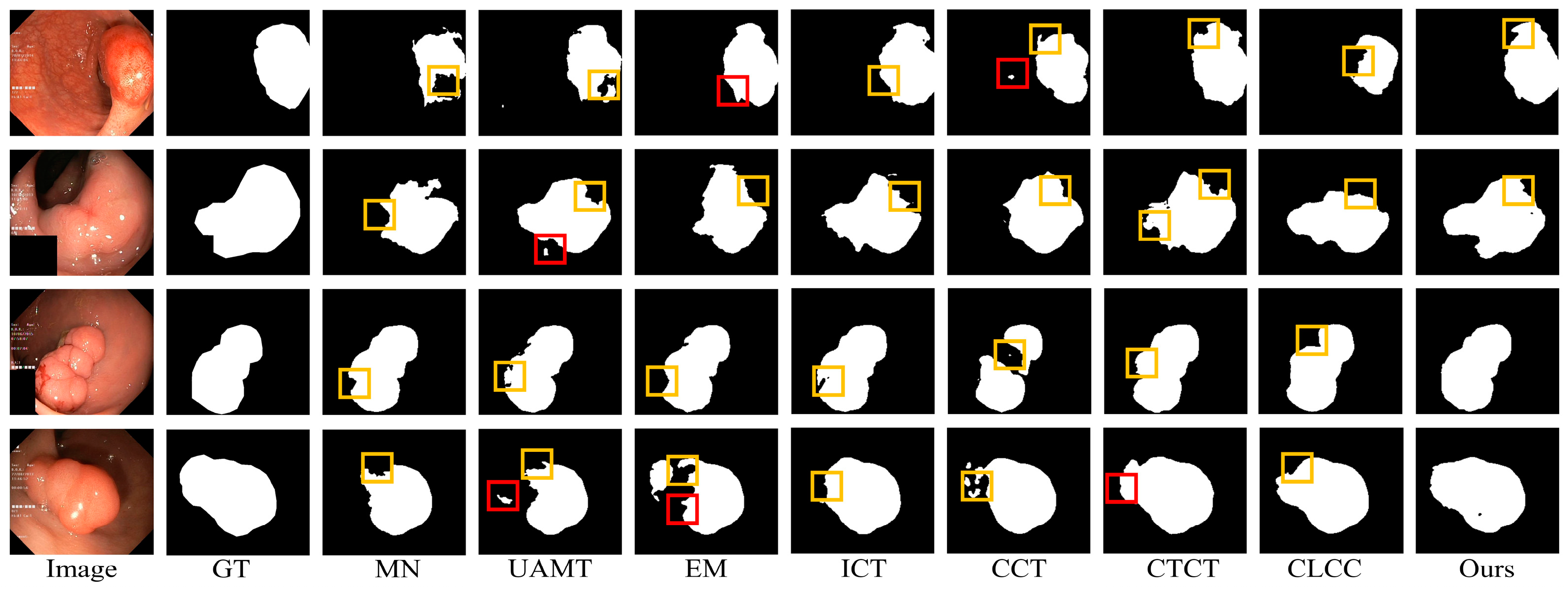
4.4.2. Comparison of the Kvasir-SEG Dataset

To study the generalization of our method, we evaluated it on the popular public Kvasir-SEG dataset for polyp segmentation. Consistent with the honeycomb lung segmentation, all other methods also used UNet as the backbone and had the same experiment settings.

The quantitative results for the different annotations (10% labeled or 20% labeled) are displayed in

Table 3. Comparison of different semi-supervised methods on the Kvasir-SEG dataset (10% labeled or 20% labeled).

Data	Methods	IoU (%)	Dice (%)	HD95	ASSD
10% Labeled	MN	53.5	64.3	31.30	7.22
	UAMT	49.9	60.5	36.06	9.09
	EM	49.4	61.4	41.16	11.24
	DAN	51.7	63.6	37.17	10.32
	ICT	55.9	67.1	32.62	7.79
	CCT	50.9	61.6	33.45	6.62
	CTCT	57.2	67.8	31.95	7.24
	CLCC	53.4	64.5	55.25	16.98
	Ours	70.0	79.3	20.72	4.34
20% Labeled	MN	63.7	73.9	24.41	5.38
	UAMT	62.6	72.9	30.66	8.58
	EM	64.9	75.0	25.56	6.83
	DAN	62.3	73.0	29.14	8.14
	ICT	67.0	76.9	24.86	6.47
	CCT	65.1	74.9	24.14	5.41
	CTCT	68.7	77.8	20.12	4.13
	CLCC	59.8	71.3	53.94	17.09
	Ours	71.1	80.3	20.498	3.22

. The experimental results indicate that our proposed method achieved the best performance with 20% annotations. The Dice, IoU, HD95, and ASSD reached 71.1%, 80.3%, 20.50, and 4.09, respectively. With 10% of the data labeled, compared with 20%, the Dice and IoU of our method decreased by 1.1% and 1.0%, respectively, while the HD95 and ASSD increased by 0.22 and 0.25. Nevertheless, our method demonstrated a superior performance compared to the other methods with less than 10% labeled.

Figure 5 shows the qualitative segmentation results of some methods with less than 20% labeled. In order to clearly observe the segmentation performance, we also used yellow and red boxes to mark those significantly missed and incorrectly detected by other methods, respectively. As we can see, our method can segment the polyp areas more accurately, with fewer missed and incorrect detections compared to other methods, further demonstrating the outstanding generalization ability of our approach for other medical data.

4.5. Grading Diagnosis Results

In order to evaluate the performance of our proposed method in grading diagnosis task, we compared the following five classic convolutional neural networks: AlexNet [56], VGG19 [57], ResNet18 [58], MobileNetV2 [59], and DenseNet121 [60]. The beforementioned classification metrics are used to measure the performance of the model, including accuracy (Acc), precision (Pre), sensitivity (Sen), and F1-score (F1). The higher values of these metrics indicate that the model’s disease grading is more accurate. The classification results are shown in

Table 4. Comparison of the classification results of different CNNs on the honeycomb lung dataset.

Methods	Acc (%)	Pre (%)	Sen (%)	F1 (%)
AlexNet	68.48	70.77	68.55	66.80
VGG19	87.17	84.54	86.43	84.33
ResNet18	87.86	85.06	85.80	84.87
MobileNetV2	87.59	85.05	87.08	84.86
DenseNet121	87.73	87.06	8.60	85.14
Ours	89.68	87.35	89.45	87.34

, and our method achieved the highest classification accuracy. Compared with the second-ranked ResNet18, our method showed improvement by 1.82%, 2.29%, 3.65%, and 2.47% on Acc, Pre, Sen, and F1, respectively, reaching 89.68%, 87.35%, 89.45%, and 84.87%. In addition, to observe the classification performance of the model for different disease grades, we visualized a confusion matrix for each method to evaluate the classification of each grade. As shown in Figure 6, the recognition accuracy of our method for grading I, grading II, and grading III reached more than 90%, which is better than the classification results of other models. It is worth noting that our method has a recognition rate of only 64.2% for grading IV, with 33% being misclassified as grading III. In our opinion, this is due to the high similarity between the lesion images of grading IV and grading III, which leads to confusion in classification. Nevertheless, it is still meaningful for the clinical grading task of honeycomb lung, as in most cases, the treatment for grading IV and grading III is consistent. In particular, to explore clinical usability, we additionally collected 210 lesion slices and invited professional physicians to evaluate the grading results. As displayed in

Table 5. The classification results on the different grades by physicians and by our method.

Grades	Ours	Physician
I	31	25
II	104	109
III	57	65
IV	18	11

, in most cases, our method can accurately grade the diseases and be consistent with the clinical diagnosis.

Furthermore, to explore the interpretability of our method for different grades of lesion in images, we visualized heatmaps for images of different grades. Figure 7 shows the regions of interest identified by our method for different grades of honeycomb lungs. Obviously, our method can accurately identify lesion regions in images of different grades. Overall, our method exhibited an excellent performance in the grading task of honeycomb lung, maintaining a high level of consistency with physician evaluations. Additionally, the heatmap analysis shows good interpretability. Thus, our method can assist physicians in correctly grading honeycomb lung.

4.6. Ablation Study

4.6.1. Ablation of Losses

To demonstrate the effectiveness of each loss term in the total loss function, we conducted ablation experiments involving supervised learning, cross-learning, global contrast, local contrast, and classification task.

Table 6. Ablation study of different loss combinations in the total loss in the honeycomb lung dataset (20% labeled).

${\mathcal{L}}_{\mathit{s}\mathit{u}\mathit{p}}$	${\mathcal{L}}_{\mathit{c}\mathit{l}\mathit{n}}$	${\mathcal{L}}_{\mathit{g}\mathit{l}\mathit{o}\mathit{b}\mathit{a}\mathit{l}\_\mathit{c}\mathit{o}\mathit{n}}$	${\mathcal{L}}_{\mathit{l}\mathit{o}\mathit{c}\mathit{a}\mathit{l}\_\mathit{c}\mathit{o}\mathit{n}}$	${\mathcal{L}}_{\mathit{c}\mathit{l}\mathit{s}}$	IoU (%)	Dice (%)	HD95	ASSD
√					66.8	78.7	9.12	1.14
√	√				71.0	82.0	7.04	1.00
√	√	√			72.2	83.0	6.30	0.98
√	√		√		72.8	83.2	6.41	0.83
√	√	√	√		73.7	84.1	6.35	0.84
√	√	√	√	√	75.6	85.5	4.95	0.77

shows the results of our ablation experiments on the honeycomb lung dataset (20% labeled). In the table, ${\mathcal{L}}_{sup}$ represents the supervised loss, ${\mathcal{L}}_{cln}$ represents the cross-learnloss ${\mathcal{L}}_{global\_con}$ and ${\mathcal{L}}_{local\_con}$ refer to the global and local contrast losses, respectively. ${\mathcal{L}}_{cls}$ denotes the classification task loss.

The results show that without adding any constraints, the model using only supervised learning has the lowest segmentation performance. As an effective learning strategy that fully extracts features from different paradigms of CNN and transformer, the addition of cross-learning significantly boosted the performance of the model compared to using only supervised learning. Then, we separately investigated the impact of global contrast loss and local contrast loss on the model. In fact, the performance of the model was further improved due to the ability of contrastive learning to learn richer feature representations. Notably, combining different levels of contrastive losses is better than using them individually. Finally, the introduction of classification loss enables our method to achieve optimal results, which demonstrates that classification task can further improve model results. Thus, each component of the total loss is effective in achieving superior performance.

4.6.2. Ablation of Shape-Edge Awareness Constraint

To verify that imposing shape-edge awareness enhances the model’s ability to recognize lesion regions and edges, we conducted an experiment on the honeycomb lung dataset (20% labeled) without imposing shape-edge awareness constraints, denoted as none. Figure 8 presents the performance of our model without imposing the shape-edge awareness. As observed, the model without the imposed constraints obtained an IoU of 73.1%, Dice of 83.7%, HD95 of 5.78, and ASSD of 0.99. In comparison, after imposing the constraints, the model’s ability to locate lesion regions and edges was improved, with the IoU, Dice coefficient, HD95, and ASSD reaching 75.6%, 85.5%, 4.95, and 0.77, respectively. Therefore, adding shape-edge awareness is an effective and simple strategy to perform more precise localization of target regions.

4.6.3. Ablation of MultiTask Architecture

To study the joint promoting effect of semi-supervised segmentation and grading diagnosis tasks, we compared the performance of grading diagnosis and semi-supervised segmentation under a single task setting.

Table 7. Ablation of multitask on segmentation results.

Methods	IoU (%)	Dice (%)	HD95	ASSD
single-seg	73.7	84.1	6.35	0.84
multitask	75.6	85.5	4.95	0.77

presents the segmentation results of the model on the honeycomb lung dataset (20% labeled) in single-task (denoted as single-seg) and multitask (denoted as multitask) settings. The results show that the model trained jointly with segmentation and classification is better than the single segmentation model in IoU, Dice, HD95, and ASSD. On the other hand, semi-supervised segmentation task also improves the performance of grading diagnosis. As shown in Figure 9, compared to the single classification task (denoted as single-cls), our multitask architecture improved the Acc, Pre, Sen, and F1 scores by 1.82%, 2.29%, 3.65, and 2.47%, respectively. Overall, the multitask architecture of semi-supervised segmentation and grading diagnosis can boost the overall performance of the model compared to a single segmentation or classification task.

5. Discussion

Honeycomb lung is a serious life-threatening disease in which the lungs exhibit classical honeycomb-like tissue. In clinical diagnosis, the treatment plan varies according to the severity level of the disease. For example, antifibrotic drugs are often used in the early stage of the disease, while lung transplantation is advocated in the later stage. Therefore, accurate diagnosis of a patient’s disease grade is necessary to prolong survival. It is worth noting that the size and extent of the lesions are crucial factors for physicians to assess the severity of the condition [61]. Inspired by this, we combined semi-supervised segmentation with grading diagnosis. In our opinion, on the one hand, semi-supervised segmentation can provide information about the size of the disease for the grading diagnosis task. On the other hand, grading diagnosis also provides auxiliary information such as the texture and severity of the lesion for the segmentation task. To the best of our knowledge, this is the first method that combines semi-supervised segmentation and grading diagnosis specifically for honeycomb lung. Concretely, in semi-supervised segmentation we first adopt a cross-learning strategy to simultaneously learn the local features and long-distance dependencies extracted by CNN and transformer. Secondly, considering the complexity of the lesion area, we designed edge-shape aware constraints to assist the model in locating the lesion area. Next, to encourage model understanding of lesion features, global contrast learning and local contrast learning are developed to capture semantic-level and pixel-level features, respectively. Lastly, for a more accurate grading diagnosis, we proposed a gradient thresholding algorithm to aggregate segmentation results.

To demonstrate the effectiveness of our approach, we compared our method with several semi-supervised segmentation algorithms and classic convolutional neural networks, including Mean Teacher (MN) [49], Uncertainty-Aware Mean Teacher (UAMT) [50], Entropy Minimization (EM) [51], Interpolation Consistency Training (ICT) [52], Deep Adversarial Networks (DAN) [53], Cross-Consistency Training (CCT) [54], Cross Teaching between CNN and transformer (CTCT) [37], Cross-level contrastive learning and consistency constraint (CLCC) [55], AlexNet [56], VGG19 [57], ResNet18 [58], MobileNetV2 [59], and DenseNet121 [60]. Experimental results show that our method achieved optimal results in both grading diagnosis and semi-supervised segmentation tasks. Specifically, in semi-supervised segmentation, we obtained 75.6% IoU, 85.5% Dice, 4.95 HD95, and 0.77 ASSD. The visualization results further illustrated that our method can more accurately segment the lesions with a lower false detection rate compared to other semi-supervised learning approaches. Our grading diagnostic network achieved 89.68% Acc, 87.35% Pre, 89.45% Sen and 87.34% F1 respectively. In particular, the network has good interpretability and is consistent with physician diagnosis in most cases.

Moreover, to verify the generalization of the segmentation method, we further tested our method on the Kvasir-SEG dataset. The quantitative results are presented in Table 3. Regardless of the proportion of labeled data, our method obtained the best segmentation results. The qualitative analysis, as shown in Figure 5, demonstrated that our method achieves more accurate localization and finer segmentation of the lesions compared to other methods. Thus, our method not only performs well in segmenting honeycomb lung, but also exhibits strong generalization capabilities for other medical images.

Finally, we investigated the effectiveness of the components in the loss function, shape-edge awareness constraint, and multitask architecture. Table 6 demonstrates that each individual loss contributes to the improvement of our model, suggesting that each component in the overall loss is beneficial for enhancing the model’s performance. The ablation results of shape-edge aware constraints are displayed in Figure 9. Compared with no constraints, our model achieved the optimal results of 75.6% IoU, 85.5% Dice, 4.945 HD95, and 0.774 ASSD. In addition, to check whether the multitask architecture can enhance the overall performance of the model, we designed separate single-task models for grading diagnosis and segmentation. As shown in Table 7 and Figure 9, compared to the single-task architecture networks, our proposed multitask architecture obtained improvements in both classification and segmentation accuracy, achieving state-of-the-art performance.

Despite our method having achieved promising results in the semi-supervised segmentation and grading diagnosis task for honeycomb lung, there are still some limitations that need to be addressed. Firstly, our method processes data in 2D slices rather than the entire 3D volume, which may cause the loss of spatial information. Next, distinguishing between grading III and grading IV images of honeycomb lung can be challenging, and it requires us to improve the accuracy of classifying grading IV images. Additionally, the lack of external validation on independent datasets increases the risk of overfitting to our specific dataset, which is limited in size. With a small dataset, the model may excessively adapt to the unique characteristics and patterns present in our training data. Finally, the dataset we have collected for honeycomb lung is limited to a single hospital, lacking data from other hospitals or regions. In the future, we plan to expand our method to 3D volume, in order to preserve more spatial context. Additionally, we will collect data from different hospitals and regions to further improve the accuracy of the model and enhance the diversity of the dataset.

6. Conclusions

In this paper, we propose a novel multitask architecture for grading diagnosis and semi-supervised segmentation of honeycomb lung. To the best of our knowledge, this is the first method to combine the above two tasks for the intelligent diagnosis of honeycomb lung. Firstly, we adapted cross-learning to obtain local information and the long-range dependencies from different paradigm features. Secondly, a simple and efficient shape-edge awareness constraint was designed to assist the model in localizing lesions. Then, we developed global and local contrast learning to capture richer semantic-level and pixel-level features in lesion images, respectively. Finally, considering that segmentation results can assist in grading diagnosis, the gradient thresholding algorithm was proposed to aggregate the segmentation results to improve the diagnostic accuracy of different grades. Extensive experiments demonstrate the superiority of our proposed method. Compared to universal semi-supervised segmentation models and classification networks, our method achieves state-of-the-art performance. Furthermore, we conducted additional segmentation experiments on Kvasir-SEG, which further indicate the excellent generalization capabilities of our method on other medical images. Notably, our method exhibits high consistency with physician diagnoses in external data experiments for grading diagnosis task. The qualitative and quantitative analyses demonstrated that our method is meaningful and efficient. It not only alleviates the burden of manual annotation but also provides intelligent assistance for honeycomb lung diagnosis. In the future, we will focus on expanding the dataset and achieving more precise predictions.

References

1. Moss, B.J.; Ryter, S.W.; Rosas, I.O. Pathogenic mechanisms underlying idiopathic pulmonary fibrosis. Annu. Rev. Pathol. Mech. Dis. 2022, 17, 515–546. [Google Scholar] [CrossRef] [PubMed]
2. Badyal, R.; Whalen, B.A.; Singhera, G.K.; Sahin, B.; Keen, K.J.; Ryerson, C.J.; Wilcox, P.; Dunne, J.V. Regulation of MicroRNA Expression in Scleroderma and Idiopathic Pulmonary Fibrosis: A Research Study. Undergrad. Res. Nat. Clin. Sci. Technol. J. 2023, 7, 1–12. [Google Scholar] [CrossRef]
3. Obi, O.N.; Alqalyoobi, S.; Maddipati, V.; Lower, E.E.; Baughman, R.P. High-Resolution CT Scan Fibrotic Patterns in Stage 4 Pulmonary Sarcoidosis: Impact on Pulmonary Function and Survival. Chest 2023, 165, 892–907. [Google Scholar] [CrossRef] [PubMed]
4. Yudin, A.L. Metaphorical Signs in Computed Tomography of Chest and Abdomen; Springer: Berlin/Heidelberg, Germany, 2014. [Google Scholar]
5. Hosseini, M.; Salvatore, M. Is pulmonary fibrosis a precancerous disease? Eur. J. Radiol. 2023, 160, 110723. [Google Scholar] [CrossRef]
6. Kunihiro, Y.; Matsumoto, T.; Murakami, T.; Shimokawa, M.; Kamei, H.; Tanaka, N.; Ito, K. A quantitative analysis of long-term follow-up computed tomography of idiopathic pulmonary fibrosis: The correlation with the progression and prognosis. Acta Radiol. 2023, 64, 2409–2415. [Google Scholar] [CrossRef] [PubMed]
7. Glass, D.S.; Grossfeld, D.; Renna, H.A.; Agarwala, P.; Spiegler, P.; DeLeon, J.; Reiss, A.B. Idiopathic pulmonary fibrosis: Current and future treatment. Clin. Respir. J. 2022, 16, 84–96. [Google Scholar] [CrossRef] [PubMed]
8. Raghu, G.; Remy-Jardin, M.; Richeldi, L.; Thomson, C.C.; Inoue, Y.; Johkoh, T.; Kreuter, M.; Lynch, D.A.; Maher, T.M.; Martinez, F.J.; et al. Idiopathic pulmonary fibrosis (an update) and progressive pulmonary fibrosis in adults: An official ATS/ERS/JRS/ALAT clinical practice guideline. Am. J. Respir. Crit. Care Med. 2022, 205, e18–e47. [Google Scholar] [CrossRef]
9. Khor, Y.H.; Bissell, B.; Ghazipura, M.; Herman, D.; Hon, S.M.; Hossain, T.; Kheir, F.; Knight, S.L.; Kreuter, M.; Macrea, M.; et al. Antacid medication and antireflux surgery in patients with idiopathic pulmonary fibrosis: A systematic review and meta-analysis. Ann. Am. Thorac. Soc. 2022, 19, 833–844. [Google Scholar] [CrossRef] [PubMed]
10. Candia, C.; Lombardi, C.; Merola, C.; Ambrosino, P.; D’anna, S.E.; Vicario, A.; De Marco, S.; Molino, A.; Maniscalco, M. The Role of High-Flow Nasal Cannula Oxygen Therapy in Exercise Testing and Pulmonary Rehabilitation: A Review of the Current Literature. J. Clin. Med. 2023, 13, 232. [Google Scholar] [CrossRef]
11. Itoh, T.; Kawasaki, T.; Kaiho, T.; Shikano, K.; Naito, A.; Abe, M.; Suzuki, H.; Ota, M.; Yoshino, I.; Suzuki, T. Long-term nintedanib treatment for progressive pulmonary fibrosis associated with Hermansky-Pudlak syndrome type 1 followed by lung transplantation. Respir. Investig. 2024, 62, 176–178. [Google Scholar] [CrossRef]
12. Lee, J.H.; Song, J.W. Diagnostic approaches for idiopathic pulmonary fibrosis. Tuberc. Respir. Dis. 2024, 87, 40–51. [Google Scholar] [CrossRef] [PubMed]
13. Nam, J.G.; Choi, Y.; Lee, S.-M.; Yoon, S.H.; Goo, J.M.; Kim, H. Prognostic value of deep learning–based fibrosis quantification on chest CT in idiopathic pulmonary fibrosis. Eur. Radiol. 2023, 33, 3144–3155. [Google Scholar] [CrossRef]
14. Oda, K.; Ishimoto, H.; Yatera, K.; Naito, K.; Ogoshi, T.; Yamasaki, K.; Imanaga, T.; Tsuda, T.; Nakao, H.; Kawanami, T.; et al. High-resolution CT scoring system-based grading scale predicts the clinical outcomes in patients with idiopathic pulmonary fibrosis. Respir. Res. 2014, 15, 10. [Google Scholar] [CrossRef] [PubMed]
15. Gang, L.; Haixuan, Z.; Linning, E.; Ling, Z.; Yu, L.; Juming, Z. Recognition of honeycomb lung in CT images based on improved MobileNet model. Med. Phys. 2021, 48, 4304–4315. [Google Scholar] [CrossRef] [PubMed]
16. Su, N.; Hou, F.; Zheng, W.; Wu, Z.; Linning, E. Computed Tomography–Based Deep Learning Model for Assessing the Severity of Patients With Connective Tissue Disease–Associated Interstitial Lung Disease. J. Comput. Assist. Tomogr. 2023, 47, 738–745. [Google Scholar] [CrossRef] [PubMed]
17. Li, G.; Xie, J.; Zhang, L.; Sun, M.; Li, Z.; Sun, Y. MCAFNet: Multiscale cross-layer attention fusion network for honeycomb lung lesion segmentation. Med. Biol. Eng. Comput. 2023, 62, 1121–1137. [Google Scholar] [CrossRef] [PubMed]
18. Jianjian, W.; Li, G.; He, K.; Li, P.; Zhang, L.; Wang, R. MCSC-UTNet: Honeycomb lung segmentation algorithm based on Separable Vision Transformer and context feature fusion. In Proceedings of the 2023 2nd Asia Conference on Algorithms, Computing and Machine Learning, Shanghai, China, 17–19 March 2023; pp. 488–494. [Google Scholar]
19. Han, K.; Sheng, V.S.; Song, Y.; Liu, Y.; Qiu, C.; Ma, S.; Liu, Z. Deep semi-supervised learning for medical image segmentation: A review. Expert Syst. Appl. 2024, 245, 123052. [Google Scholar] [CrossRef]
20. Jiao, R.; Zhang, Y.; Ding, L.; Xue, B.; Zhang, J.; Cai, R.; Jin, C. Learning with limited annotations: A survey on deep semi-supervised learning for medical image segmentation. Comput. Biol. Med. 2023, 169, 107840. [Google Scholar] [CrossRef] [PubMed]
21. Arazo, E.; Ortego, D.; Albert, P.; O’Connor, N.E.; McGuinness, K. Pseudo-labeling and confirmation bias in deep semi-supervised learning. In Proceedings of the 2020 International Joint Conference on Neural Networks (IJCNN), Glasgow, UK, 19–24 July 2020; IEEE: Piscataway, NJ, USA, 2020; pp. 1–8. [Google Scholar]
22. Wu, J.; Fan, H.; Zhang, X.; Lin, S.; Li, Z. Semi-supervised semantic segmentation via entropy minimization. In Proceedings of the 2021 IEEE International Conference on Multimedia and Expo (ICME), Shenzhen, China, 5–9 July 2021; IEEE: Piscataway, NJ, USA, 2021; pp. 1–6. [Google Scholar]
23. Fan, Y.; Kukleva, A.; Dai, D.; Schiele, B. Revisiting consistency regularization for semi-supervised learning. Int. J. Comput. Vis. 2023, 131, 626–643. [Google Scholar] [CrossRef]
24. Wang, K.; Zhan, B.; Zu, C.; Wu, X.; Zhou, J.; Zhou, L.; Wang, Y. Semi-supervised medical image segmentation via a tripled-uncertainty guided mean teacher model with contrastive learning. Med. Image Anal. 2022, 79, 102447. [Google Scholar] [CrossRef]
25. Liu, Z.; Wu, F.; Wang, Y.; Yang, M.; Pan, X. FedCL: Federated Contrastive Learning for Multi-center Medical Image Classification. Pattern Recognit. 2023, 143, 109739. [Google Scholar] [CrossRef]
26. Liu, P.; Zheng, G. Context-aware voxel-wise contrastive learning for label efficient multi-organ segmentation. In Proceedings of the International Conference on Medical Image Computing and Computer-Assisted Intervention, Singapore, 18–22 September 2022; Springer: Berlin/Heidelberg, Germany, 2022; pp. 653–662. [Google Scholar]
27. Chen, X.; Yuan, Y.; Zeng, G.; Wang, J. Semi-supervised semantic segmentation with cross pseudo supervision. In Proceedings of the IEEE/CVF Conference on Computer Vision and Pattern Recognition, Nashville, TN, USA, 20–25 June 2021; pp. 2613–2622. [Google Scholar]
28. Liu, J.; Desrosiers, C.; Zhou, Y. Semi-supervised medical image segmentation using cross-model pseudo-supervision with shape awareness and local context constraints. In International Conference on Medical Image Computing and Computer-Assisted Intervention; Springer: Berlin/Heidelberg, Germany, 2022; pp. 140–150. [Google Scholar]
29. Sarkar, S.; Min, K.; Ikram, W.; Tatton, R.W.; Riaz, I.B.; Silva, A.C.; Bryce, A.H.; Moore, C.; Ho, T.H.; Sonpavde, G.; et al. Performing Automatic Identification and Staging of Urothelial Carcinoma in Bladder Cancer Patients Using a Hybrid Deep-Machine Learning Approach. Cancers 2023, 15, 1673. [Google Scholar] [CrossRef] [PubMed]
30. Dinesh, M.G.; Bacanin, N.; Askar, S.S.; Abouhawwash, M. Diagnostic ability of deep learning in detection of pancreatic tumour. Sci. Rep. 2023, 13, 9725. [Google Scholar] [CrossRef]
31. Zheng, Y.-M.; Che, J.-Y.; Yuan, M.-G.; Wu, Z.-J.; Pang, J.; Zhou, R.-Z.; Li, X.-L.; Dong, C. A CT-based deep learning radiomics nomogram to predict histological grades of head and neck squamous cell carcinoma. Acad. Radiol. 2023, 30, 1591–1599. [Google Scholar] [CrossRef] [PubMed]
32. Lu, L.; Yin, M.; Fu, L.; Yang, F. Uncertainty-aware pseudo-label and consistency for semi-supervised medical image segmentation. Biomed. Signal Process. Control 2023, 79, 104203. [Google Scholar] [CrossRef]
33. Berthelot, D.; Carlini, N.; Goodfellow, I.; Papernot, N.; Oliver, A.; Raffel, C.A. Mixmatch: A holistic approach to semi-supervised learning. Adv. Neural Inf. Process. Syst. 2019, 32. [Google Scholar]
34. Li, S.; Zhang, Y.; Yang, X. Semi-supervised cardiac mri segmentation based on generative adversarial network and variational auto-encoder. In 2021 IEEE International Conference on Bioinformatics and Biomedicine (BIBM); IEEE: Piscataway, NJ, USA, 2021; pp. 1402–1405. [Google Scholar]
35. Zhang, J.; Zhang, S.; Shen, X.; Lukasiewicz, T.; Xu, Z. Multi-ConDoS: Multimodal contrastive domain sharing generative adversarial networks for self-supervised medical image segmentation. IEEE Trans. Med. Imaging 2023, 43, 76–95. [Google Scholar] [CrossRef]
36. Fu, S.; Liu, W.; Zhang, K.; Zhou, Y.; Tao, D. Semi-supervised classification by graph p-Laplacian convolutional networks. Inf. Sci. 2021, 560, 92–106. [Google Scholar] [CrossRef]
37. Luo, X.; Hu, M.; Song, T.; Wang, G.; Zhang, S. XLuo; Hu, M.; Song, T.; Wang, G.; Zhang, S. Semi-supervised medical image segmentation via cross teaching between cnn and transformer. In Proceedings of the International Conference on Medical Imaging with Deep Learning, PMLR, Zurich, Switzerland, 6–8 July 2022; pp. 820–833. [Google Scholar]
38. Lai, X.; Tian, Z.; Jiang, L.; Liu, S.; Zhao, H.; Wang, L.; Jia, J. Semi-supervised semantic segmentation with directional context-aware consistency. In Proceedings of the IEEE/CVF Conference on Computer Vision and Pattern Recognition, Nashville, TN, USA, 20–25 June 2021; pp. 1205–1214. [Google Scholar]
39. Abramovich, O.; Pizem, H.; Van Eijgen, J.; Oren, I.; Melamed, J.; Stalmans, I.; Blumenthal, E.Z.; Behar, J.A. FundusQ-Net: A regression quality assessment deep learning algorithm for fundus images quality grading. Comput. Methods Programs Biomed. 2023, 239, 107522. [Google Scholar] [CrossRef]
40. Liawrungrueang, W.; Kim, P.; Kotheeranurak, V.; Jitpakdee, K.; Sarasombath, P. Automatic detection, classification, and grading of lumbar intervertebral disc degeneration using an artificial neural network model. Diagnostics 2023, 13, 663. [Google Scholar] [CrossRef]
41. Rastogi, D.; Johri, P.; Tiwari, V.; Elngar, A.A. Multi-class classification of brain tumour magnetic resonance images using multi-branch network with inception block and five-fold cross validation deep learning framework. Biomed. Signal Process. Control 2024, 88, 105602. [Google Scholar] [CrossRef]
42. Batra, K.; Adams, T.N. Imaging features of idiopathic interstitial lung diseases. J. Thorac. Imaging 2023, 38, S19–S29. [Google Scholar] [CrossRef]
43. Zhang, Y.; Yang, Q. A survey on multi-task learning. IEEE Trans. Knowl. Data Eng. 2021, 34, 5586–5609. [Google Scholar] [CrossRef]
44. Wu, W.; Yan, J.; Zhao, Y.; Sun, Q.; Zhang, H.; Cheng, J.; Liang, D.; Chen, Y.; Zhang, Z.; Li, Z.-C. Multi-task learning for concurrent survival prediction and semi-supervised segmentation of gliomas in brain MRI. Displays 2023, 78, 102402. [Google Scholar] [CrossRef]
45. Zeng, L.-L.; Gao, K.; Hu, D.; Feng, Z.; Hou, C.; Rong, P.; Wang, W. SS-TBN: A Semi-Supervised Tri-Branch Network for COVID-19 Screening and Lesion Segmentation. IEEE Trans. Pattern Anal. Mach. Intell. 2023, 45, 10427–10442. [Google Scholar] [CrossRef] [PubMed]
46. Liu, Y.; Wang, W.; Luo, G.; Wang, K.; Li, S. A contrastive consistency semi-supervised left atrium segmentation model. Comput. Med Imaging Graph. 2022, 99, 102092. [Google Scholar] [CrossRef]
47. Ronneberger, O.; Fischer, P.; Brox, T. U-net: Convolutional networks for biomedical image segmentation. In Proceedings of the Medical Image Computing and Computer-Assisted Intervention–MICCAI 2015: 18th International Conference, Munich, Germany, 5–9 October 2015; pp. 234–241. [Google Scholar]
48. Cao, H.; Wang, Y.; Chen, J.; Jiang, D.; Zhang, X.; Tian, Q.; Wang, M. Swin-unet: Unet-like pure transformer for medical image segmentation. In Proceedings of the European Conference on Computer Vision 2022, Tel Aviv, Israel, 23–27 October 2022; Springer: Berlin/Heidelberg, Germany, 2022; pp. 205–218. [Google Scholar]
49. Tarvainen, A.; Valpola, H. Mean teachers are better role models: Weight-averaged consistency targets improve semi-supervised deep learning results. Adv. Neural Inf. Process. Syst. 2017, 30, 1196–1205. [Google Scholar]
50. Yu, L.; Wang, S.; Li, X.; Fu, C.-W.; Heng, P.-A. Uncertainty-aware self-ensembling model for semi-supervised 3D left atrium segmentation. In Proceedings of the Medical Image Computing and Computer Assisted Intervention–MICCAI 2019: 22nd International Conference, Shenzhen, China, 13–17 October 2019; pp. 605–613. [Google Scholar]
51. Grandvalet, Y.; Bengio, Y. Semi-supervised learning by entropy minimization. Adv. Neural Inf. Process. Syst. 2004, 17. [Google Scholar]
52. Verma, V.; Lamb, A.; Kannala, J.; Bengio, Y.; Lopez-Paz, D. Interpolation consistency training for semi-supervised learning. Neural Netw. 2022, 145, 90–106. [Google Scholar] [CrossRef]
53. Zhang, Y.; Yang, L.; Chen, J.; Fredericksen, M.; Hughes, D.P.; Chen, D.Z. Deep adversarial networks for biomedical image segmentation utilizing unannotated images. In Proceedings of the Medical Image Computing and Computer Assisted Intervention—MICCAI 2017: 20th International Conference, Quebec City, QC, Canada, 11–13 September 2017; pp. 408–416. [Google Scholar]
54. Ouali, Y.; Hudelot, C.; Tami, M. Semi-supervised semantic segmentation with cross-consistency training. In Proceedings of the IEEE/CVF Conference on Computer Vision and Pattern Recognition, Seattle, WA, USA, 13–19 June 2020; pp. 12674–12684. [Google Scholar]
55. Zhao, X.; Fang, C.; Fan, D.-J.; Lin, X.; Gao, F.; Li, G. Cross-level contrastive learning and consistency constraint for semi-supervised medical image segmentation. In Proceedings of the 2022 IEEE 19th International Symposium on Biomedical Imaging (ISBI), Kolkata, India, 28–31 March 2022; IEEE: Piscataway, NJ, USA, 2022; pp. 1–5. [Google Scholar]
56. Krizhevsky, A.; Sutskever, I.; Hinton, G.E. Imagenet classification with deep convolutional neural networks. Adv. Neural Inf. Process Syst. 2012, 2, 1097–1105. [Google Scholar] [CrossRef]
57. Simonyan, K.; Zisserman, A. Very deep convolutional networks for large-scale image recognition. arXiv 2014, arXiv:1409.1556. [Google Scholar]
58. He, K.; Zhang, X.; Ren, S.; Sun, J. Deep residual learning for image recognition. In Proceedings of the IEEE Conference on Computer Vision and Pattern Recognition, Las Vegas, NV, USA, 26 June–1 July 2016; pp. 770–778. [Google Scholar]
59. Sandler, M.; Howard, A.; Zhu, M.; Zhmoginov, A.; Chen, L.-C. Mobilenetv2: Inverted residuals and linear bottlenecks. In Proceedings of the IEEE Conference on Computer Vision and Pattern Recognition, Salt Lake City, UT, USA, 18–23 June 2018; pp. 4510–4520. [Google Scholar]
60. Huang, G.; Liu, Z.; Van Der Maaten, L.; Weinberger, K.Q. Densely connected convolutional networks. In Proceedings of the IEEE Conference on Computer Vision and Pattern Recognition, Honolulu, HI, USA, 21–26 July 2017; pp. 4700–4708. [Google Scholar]
61. Shin, S.; King, C.S.; Puri, N.; Shlobin, O.A.; Brown, A.W.; Ahmad, S.; Weir, N.A.; Nathan, S.D. Pulmonary artery size as a predictor of outcomes in idiopathic pulmonary fibrosis. Eur. Respir. J. 2016, 47, 1445–1451. [Google Scholar] [CrossRef] [PubMed]
Figure 1. CT manifestations of honeycomb lungs with different grades.
Electronics 13 02115 g001
Figure 2. Overview of the model.
Electronics 13 02115 g002
Figure 3. The construction of positive and negative pairs for different levels of contrastive learning: (a) global contrastive learning; (b) local contrastive learning.
Electronics 13 02115 g003
Figure 4. Visualization results of different semi-supervised methods on the honeycomb lung dataset (20% labeled). The yellow and red boxes represent lesions that are missed and incorrectly detected by other methods, respectively.
Electronics 13 02115 g004
Figure 5. Visualization results of different semi-supervised methods on the Kvasir-SEG dataset (20% labeled). The yellow and red boxes represent lesions that were missed and incorrectly detected by other methods, respectively.
Electronics 13 02115 g005
Figure 6. Confusion matrices: (a) our method; (b) AlexNet; (c) VGG19; (d) ResNet18; (e) DenseNet121; (f) MobileNetV2.
Electronics 13 02115 g006
Figure 7. Heatmap visualization of different grading lesion images by our method.
Electronics 13 02115 g007
Figure 8. Ablation results of shape-edge awareness constraint.
Electronics 13 02115 g008
Figure 9. Ablation of multitasks on classification results.
Electronics 13 02115 g009