A State-Feedback Control Strategy Based on Grey Fast Finite-Time Sliding Mode Control for an H-Bridge Inverter with LC Filter Output

Abstract

An H-bridge inverter with LC (inductor-capacitor) filter output allows the conversion of DC (direct current) power to AC (alternating current) power that has been used in a variety of applications, such as uninterruptible power supplies, AC motor drives, and renewable energy source systems. The fast finite-time sliding mode control (FFTSMC) features acceleration of the system state towards the equilibrium position as well as conserving insensitivity against internal parameter fluctuations as well as external load disturbances falling within the predetermined bounds. However, the FFTSMC would potentially witness chattering or steady-state errors as indefinite margins come to be exaggerated or underestimated. The chattering in the sliding mode control practice is oscillatory defective behavior. It induces inefficient operation, higher switching power losses in the transistor circuits, as well as saturated actuators, thus impairing the inverter’s output energy efficiency and raising harmonic distortion. Therefore, this paper presents the H-bridge inverter with LC filter output, which is controlled by a grey prediction fast finite-time sliding mode trajectory tracking. A more highly accurate grey prediction model based on the centered approximation methodology is deployed to vanish the chattering as well as steady-state errors. Taking into account the union of grey prediction and FFTSMC, a feedback-controlled H-bridge inverter with LC filter output allows attaining a highly efficient as well as quality sine-wave output voltage. The presented state-feedback control strategy is robust, less complex, attains more rapid convergence, and is highly accurate. The design process, computer simulation, as well as experimental results of the proposed state-feedback control strategy established that the H-bridge inverter with LC filter output has the capability to exhibit fast dynamic response time as well as good steady-state tracking behavior of the output voltage under step-loading changes and nonlinear loading conditions.

1. Introduction

H-bridge inverters with LC (inductor-capacitor) filters output have found wider application in solar photovoltaic, wind, as well as fuel cell power generation systems [1,2,3,4,5,6]. High-performance H-bridge inverters with LC filters output must provide high-quality AC (alternating current) output voltage, fast dynamic characteristics, and low levels of total harmonic distortion (THD), even under high non-linear loads. To meet these requirements, the scientific literature considers various control schemes, such as hysteresis control, cascaded repetitive control, and linear quadratic regulator (LQR) controller [7,8,9,10,11,12]. A hysteresis current control method can be introduced in the inverter with constant switching frequency. Despite the fact that such a method offers faster reaction time and higher accuracy of current tracking, the harmonics at the steady-state output should continue to be improved [7]. Application of FPGA (field programmable gate array) implementation with hysteresis current control strategy for an induction motor powered by a voltage source inverter was developed. The performance under steady-state and transient conditions proved to be satisfactory; the analog and digital signal processor with both software and hardware layouts result in relatively expensive production costs [8]. A cascade-type repetitive controller exploits the mechanism of phase cancellation to optimize a repetitive controller’s behavior for use in constant-voltage constant-frequency pulse-width-modulated DC–AC converters. The output response under non-linear loads appears to be robust, while the transient compensation lacks the desired quality [9]. Coupling the advantages of proportional-integral controller and repetitive controller to form a cascaded repetitive controller has been suggested. In comparison with the conventional parallel repetitive controller, the proposed inverter provides increased performance, but the control method becomes sophisticated [10]. There is a LQR-based voltage controller presented for grid-connected inverters applicable within the black start period. Its adjustment process allows stabilization across a variety of grid impedances. Its tuning process can be stabilized under various grid impedances. Nevertheless, the LQR depends heavily on exact system modeling [11]. With an optimized closed-loop control scheme on the basis of LQR principle, it was developed to afford both sound transient and steady-state performance of resonant inverters. There is a requirement to simplify the higher-order dimension into lower-order, which would enable the Riccati equation to be addressed [12]. In addition, proportional-integral-derivative (PID) controllers have been widely used in industry due to their simple control structure and ease of design. But the PID controller is unable to provide good control performance under highly nonlinear load disturbances, resulting in unsatisfactory transience and steady-state characteristics [13,14,15,16].

Sliding mode control (SMC) has a high degree of design simplicity and easy-to-construct models, especially its ability to resist changes in internal parameters of controlled devices and external load disturbances during sliding motion [17,18,19]. More importantly, in the application of sliding mode control, there are a lot of references to show its effective use [20,21,22,23,24]. A switched-inductor quasi-Z-source inverter was presented together with its control adopting a sliding mode control mechanism to cope with unpredictability. It gave a strong response; however, the speed of state convergence remained weak [20]. The saturated function based on the boundary was suggested, and a modified observer based on particle swarm optimization is available for estimation of the inductor current. Although such a strategy applied to DC–AC inverters enhances the transient response, the steady-state performance needs to be strengthened [21]. The use of an equivalent function in the SMC was introduced, and the robustness of the voltage source inverter can be potentially increased via integral sliding manifold; remarkably, the dynamic response was not satisfactory, even though the chatter, THD, and power factor were improved [22]. There was a suggested integral sliding mode control applied to control the switched boost inverters. The dynamic response can be accelerated while the steady-state response gains considerable improvement, whereas the dual-loop control structure complicates the algorithms [23]. The discretized version of a variable structure control scheme was introduced for single-phase T-type inverters. Even though the proposed approach can establish a low THD, its complexity in eliminating chattering increases the difficulty of future implementations compared to the simplicity of using a smoothing function [24]. It should be emphasized that under the traditional sliding mode control, the state convergence will tend to be asymptomatic for a long time, but it will not happen in a short time, which will lead to the emergence of experimental chattering phenomenon.

The recently developed fast finite-time sliding mode control (FFTSMC) originated from the concept of terminal attractors [25,26,27,28,29,30,31], it holds the insensitivity to unknown disturbances, and more notably, it accelerates the movement of the state to the equilibrium point in a limited time [32,33,34,35,36]. This control form of sliding mode greatly expands the dynamic and steady-state response of the controlled plant, except for overestimating or underestimating the boundary due to strong uncertainty, which will still lead to chattering or steady-state error. Chattering is a harmful state with the occurrence of high-frequency oscillation. Its motion on the sliding surface leads to the reduction of control accuracy, unmodeled high-frequency plant dynamics, saturation of the actuator, shortened service life, high harmonic distortion of H-bridge inverter with LC filter output, and reduced working efficiency. In order to eliminate chattering, many technical methods have been developed, such as adaptive control, hybrid strategy with adaptive control and observer method, and linear matrix inequality [37,38,39]. All these technologies can solve the chattering problem and enhance the steady-state and the transient process under disturbances, but their implementation brings some difficulties related to the high computational complexity of the algorithm. Grey prediction is widely used in various fields with the characteristics of requiring only at least four sampling data points, modeling simplicity, and uncomplicated computation [40,41,42,43,44,45,46,47]. In real work, the typical grey system is usually developed for forecasting relatively smoothed data, which varies in an exponential tendency. It has relatively little ability to forecast the randomness associated with widely varying amounts of data. An improved grey prediction (IGP) featuring a grey prediction model based on a centered approximation methodology is available to address the weaknesses of classical grey prediction towards higher forecasting quality [48,49,50,51,52]. Therefore, an IGP is employed to eliminate chattering or steady-state error, even though the uncertainty of H-bridge inverter with LC filter output may be exaggerated or underestimated. Due to the synthetic integration of the proposed state-feedback control strategy and H-bridge inverter with LC filter output, a highly efficient alternating current output voltage with very low distortion can be realized. The proposed state-feedback control strategy is helpful to improve intelligibility and simplification, ease modeling, prevent chattering, and accelerate the convergence of tracking error trajectory. In order to prove the effectiveness of the presented state-feedback control strategy, simulation results and hardware experiments are provided. The contribution of this paper can be summarized as follows: (i) The proposed FFTSMC permits a finite-time singularity-free state convergence to the equilibrium in the sliding phase, while it brings the state behavior to the sliding surface more quickly in the arrival phase. (ii) Despite the occurrence of system uncertainties, the improved grey prediction model provides a more accurate prediction of the state points. Thus, chattering and steady-state error can be suppressed, leading to a fast and stable convergence of the state trajectory towards the equilibrium point. (iii) With improved grey prediction model and the FFTSMC, the H-bridge inverter with LC filter output can yield fast dynamics and robust steady-state response under various load cases, such as sudden step-load changes and rectified loads. In terms of innovations, the proposed state-feedback control strategy is designed by considering two conditions, which are close to and far away from the sliding surface; this ensures that the system trajectory can make a quick response according to occupied state, which improves the approaching speed and the system robustness. The output-voltage THD, voltage drop, and voltage swell of the proposed H-bridge inverter with LC filter output surpass the standards of IEEE (Institute of Electrical and Electronics Engineers) and IEC (International Electrotechnical Commission). Therefore, this paper can considered as a source of reference information for researchers of H-bridge inverter with LC filter output and related control technologies.

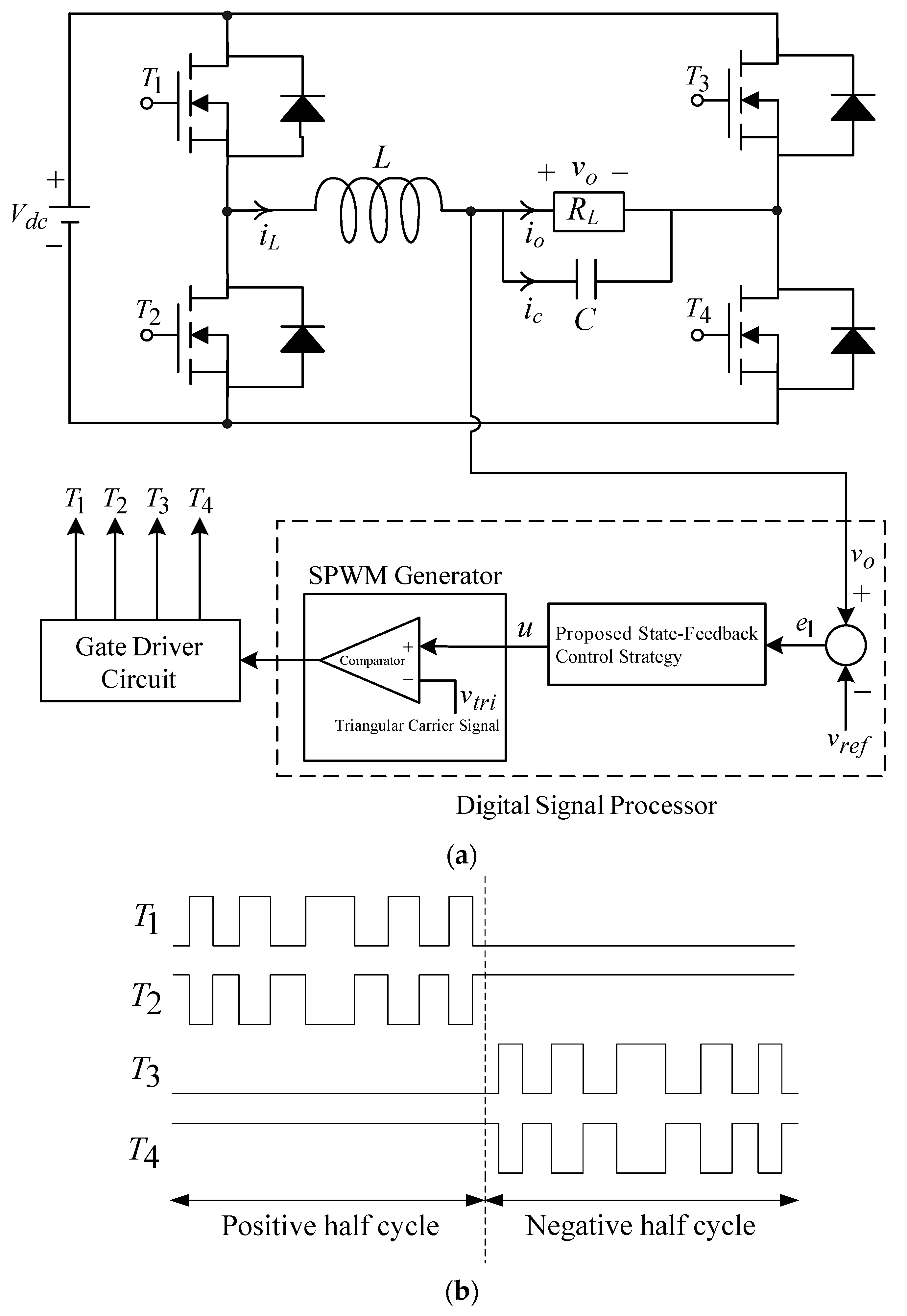
2. Modeling Description of H-Bridge Inverter with LC Filter Output

Figure 1a shows an H-bridge inverter with LC filter output, which consists of three key units: a transistor switching element, an inductive capacitive low-pass filter, and a connected load. Figure 1b shows the gate control signal generated by comparing the sinusoidal reference waveform with the high-frequency triangular carrier waveform corresponding to the H-bridge inverter with LC filter output circuit. Thereafter, the DC-link voltage is defined as $V_{dc}$, $R_L$ denotes the resistive load, and the output voltage and current can be denoted as $v_o$ and $i_o$, respectively. Applying Kirchhoff’s law to analyze the voltage and current in Figure 1a and setting the state variables $x_1=v_o$ and $x_2={\dot{v}}_o$, the state behavior of the H-bridge inverter with LC filter output can be represented as follows:

$$\left\{\begin{array}{l}{\dot{x}}_1=x_2\\ {\dot{x}}_2=-\frac{1}{LC}{x}_1-\frac{1}{R_{L}C}{x}_2+\frac{K_{spwm}}{LC}u\end{array}\right.$$

(1)

where $K_{spwm}=\frac{V_{dc}}{{\widehat{v}}_{tri}}$ represents the scaled constant gain of the inverter, ${\widehat{v}}_{tri}$ represents the amplitude of the triangular carrier signal, and $u$ shown in Figure 1a is a control signal. The $u$ has to be compared with triangular carrier signal $v_{tri}$ for the generation of SPWM (sinusoidal pulse width modulation) signals controlling the inverter switches.

The design task of an H-bridge inverter with LC filter output is a typical servo control task. Due to the fact that the output voltage of the H-bridge inverter with LC filter output is in the sine wave form of AC, it is necessary to track the required AC reference form $v_{r\_AC}=\sqrt{2}{V}_{rms}\cdot \sin (\omega t)$, where $V_{rms}$ is the root mean square value, and $\omega$ is the angular frequency. Therefore, based on the relationship between (1) and $v_{r\_AC}$, the error state variables can be defined as follows:

$$\left\{\begin{array}{c}{e}_1=x_1-v_{r\_AC}\\ e_2=x_2-{\dot{v}}_{r\_AC}\end{array}\right.$$

(2)

Furthermore, utilizing (1) and (2), one can write the error equation of state for the H-bridge inverter with LC filter output in the following way:

$$\left\{\begin{array}{l}{\dot{e}}_1=e_2\\ {\dot{e}}_2=a_1{e}_1+a_2{e}_2+b_{p}u+\psi \end{array}\right.$$

(3)

where $a_1=-1/LC$, $a_2=-1/R_{L}C$, and $b_p=K_{spwm}/LC$, and $\psi =-a_1{v}_{r\_AC}-a_2{\dot{v}}_{r\_AC}-{\ddot{v}}_{r\_AC}$ specifies disruptions caused by step-load changes or nonlinear loading conditions. The $u$ displayed in (3) is capable of creating a tracking behavior that tends to zero. That is, the FFTSMC is devised to run the output voltage of H-bridge inverter with LC filter output, which allows the error trajectory to zero by tracking the AC referenced voltage for a shorter time. A grey prediction model based on the centered approximation methodology serves to mitigate chattering or steady-state error when the uncertainty margin is evaluated too high or low; this guarantees a highly efficient, good quality sine voltage output for an H-bridge inverter with LC filter output. The control design is illustrated as well as deduced in the following section.

3. Control Design

In this section, we first illustrate the problem of a nonlinear system (as in (3)) presented using the traditional finite-time sliding mode control (FTSMC). A suggested sliding mode control law (i.e., FFTSMC) is first designed. The traditional FTSMC is considered as follows:

$$S=e_2+\xi e_1^{{\kappa }_2/{\kappa }_1}$$

(4)

where $\xi >0$, and both ${\kappa }_1$ and ${\kappa }_2$ are positive odd integers, satisfying ${\kappa }_1>{\kappa }_2$. Once the sliding variables in (4) arrives at the $S=0$, the behavior of the system can be characterized by $e_2={\dot{e}}_1=-\xi e_1^{{\kappa }_2/{\kappa }_1}$. It takes a finite time $t_f$ for the evolution from a non-zero value (arbitrary initial state $e_1(0)\ne 0$) to zero as follows: $t_f=\frac{1}{\xi (1-{\kappa }_2/{\kappa }_1)}{\left|e_1(0)\right|}^{1-{\kappa }_2/{\kappa }_1}$. Thus, the state of the system will converge to zero in a finite amount of time, but a singularity is generated under $e_1=0$, $e_2\ne 0$, and $0<{\kappa }_2/{\kappa }_1<1$, causing the closed-loop instability.

Thus, regarding the error equation of state (3), the sliding surface necessary to ensure fast time convergence without singularity can be expressed as follows:

$$s=e_1+\beta e_2^{{\alpha }_2/{\alpha }_1}$$

(5)

where $\beta >0$, and ${\alpha }_1$ and ${\alpha }_2$ are positive odd numbers, bounded by $1<{\alpha }_2/{\alpha }_1<2$.

In order to quickly enter the sliding surface, the law of reaching the sliding mode is designed below:

$$\dot{s}=-{\gamma }_1{\left|s\right|}^{{\tau }_1}(s/\left|s\right|+\epsilon )-{\gamma }_2{\left|s\right|}^{{\tau }_2}{\tanh }^{-1}(s/\mu )-{\gamma }_{3}s$$

(6)

where ${\gamma }_1>0$, ${\gamma }_2>0$, ${\gamma }_3>0$, ${\tau }_1>0$, $0<{\tau }_2<1$, and $\epsilon$ as well as $\mu$ represent small values that are greater than zero.

According to (3)–(6), the FFTSMC control law $u$ stipulates the following:

$$u=-b_p^{-1}[a_1{e}_1+a_2{e}_2+\frac{{\alpha }_1}{\beta {\alpha }_2}{e}_2^{{\alpha }_2/{\alpha }_1}+{\gamma }_1{\left|s\right|}^{{\tau }_1}(s/\left|s\right|+\epsilon )+{\gamma }_2{\left|s\right|}^{{\tau }_2}{\tanh }^{-1}(s/\mu )+{\gamma }_{3}s]$$

(7)

Proof. 

There is a candidate for defining the Lyapunov function below:

$$V=s^2/2$$

(8)

The derivative $V$ with time can be found making use of the following behavior (1) and the control law (4):

$$\begin{array}{l}\dot{V}=s\dot{s}\\ \hspace{1em}=s{\left(e_1+\beta e_2^{{\alpha }_2/{\alpha }_1}\right)}^{\prime }\\ \hspace{1em}\le -s\cdot [{\gamma }_1{\left|s\right|}^{{\tau }_1}(s/\left|s\right|+\epsilon )+{\gamma }_2{\left|s\right|}^{{\tau }_2}{\tanh }^{-1}(s/\mu )+{\gamma }_{3}s]\end{array}$$

(9)

As can be expected from (9), $s$ as well as $e_2$ cannot in any way lead to zero, for which reason $\dot{V}$ is below zero. This implies that $s$ and its derivative define the states quickly converging to the equilibrium during a finite time, in which (9) satisfies Lyapunov’s stability theorem. As a result, the dynamics of the system (3) will also have to converge quickly to the equilibrium state within a finite period of time when the control law (7) condition is applied. Remarkably, the finite-time convergence of $s$ has been proven in literature references [53,54,55], where there is a finite time $t_r=({\alpha }_2{\left|e_1(0)\right|}^{1-{\alpha }_1/{\alpha }_2})/({\beta }^{{\alpha }_1/{\alpha }_2}({\alpha }_2-{\alpha }_1))$ for the state to reach the equilibrium point. Similarly, $\dot{s}$ allows the state to arrive at the sliding surface quickly within a finite time and is explained as follows: The state trajectory arriving at the sliding surface can be distinguished into two periods. One is the item $-{\gamma }_1{\left|s\right|}^{{\tau }_1}(s/\left|s\right|+\epsilon )$ representing the quality of dynamic behavior for the state trajectory nearing the sliding surface. If the ${\gamma }_1$ becomes larger, the approaching speed tends to be faster with increased jitter; if a smaller ${\tau }_1$ is used, there is less jitter, but a slower approaching speed is achieved. The other item is $-{\gamma }_2{\left|s\right|}^{{\tau }_2}{\tanh }^{-1}(s/\mu )$, which shows the quality of dynamic behavior when the state trajectory moves away from the sliding surface. If the ${\gamma }_2$ increases, it will lead to faster approaching speed, but the jitter rises; if the ${\tau }_2$ reduces, the jitter vibration becomes smaller, but there is a reduction in the approaching speed. The item $-{\gamma }_{3}s$ allows to finely modify the approaching speed of the above two items. When the ${\gamma }_3$ increases, it is possible to have a state trajectory close to the sliding surface. The $(s/\left|s\right|+\epsilon )$ and ${\tanh }^{-1}(s/\mu )$ play the role of the smooth function, which helps to reduce the excessive amplitude of the input signal. Because a load varies in step or becomes strictly a non-linearity from (3), the chattering effect arises more drastically. To handle such a problem, an improved grey prediction method (grey prediction model based on the centered approximation methodology) is introduced in the following. It is useful for forecasting the output voltage by improved grey prediction. Based on no less than four output voltage levels, one state of the next output voltage can be forecasted. □

• Step 1: The assumption is that the initial series of data ${\mathsf{{\rm X}}}^{(0)}$ (output voltage level) is represented as follows:

  $${\mathsf{{\rm X}}}^{(0)}=\left\{{\mathsf{{\rm X}}}^{(0)}(1),{\mathsf{{\rm X}}}^{(0)}(2),\cdots ,{\mathsf{{\rm X}}}^{(0)}(\mathcal{l})\right\}$$

  (10)

  where $\mathcal{l}$ represents the amount of data. Generally, a sequence showing changes in output voltage information can be constructed using fewer (at least four) past data points.
• Step 2: There may be either positivity or negativity in the series of data, where mapped generating operation (MGO) takes place to put the primary series of data ${\mathsf{{\rm X}}}^{(0)}$ to non-negativity series ${\mathsf{{\rm X}}}_m^{(0)}$:

  $${\mathsf{{\rm X}}}_m^{(0)}=\mathrm{MGO}({\mathsf{{\rm X}}}^{(0)}(k))=\eta +\sigma {\mathsf{{\rm X}}}^{(0)}(k),k=1,2,\mathcal{l}$$

  (11)

  where both $\eta$ and $\sigma$ are greater than zero.
• Step 3: The equation for accumulated generating operation (AGO) can be formulated as follows:

  $${\mathsf{{\rm X}}}^{(1)}=\left\{{\mathsf{{\rm X}}}^{(1)}(1),{\mathsf{{\rm X}}}^{(1)}(2),\cdots ,{\mathsf{{\rm X}}}^{(1)}(j)\right\}$$

  (12)

  where ${\mathsf{{\rm X}}}^{(1)}(n)={\displaystyle \sum _{i=1}^n{\mathsf{{\rm X}}}_m^{(0)}(i)}$, $n=1,2,\cdots ,j$.
• Step 4: Taking the power of ${\rho }^{-1}$ for ${\mathsf{{\rm X}}}^{(1)}(n)$ in (12) to attenuate the sequential random uncertainty yields the following:

  $${\mathsf{{\rm X}}}^{{\rho }^{-1}}=\left\{{\mathsf{{\rm X}}}^{{\rho }^{-1}}(1),{\mathsf{{\rm X}}}^{{\rho }^{-1}}(2),\cdots ,{\mathsf{{\rm X}}}^{{\rho }^{-1}}(j)\right\}$$

  (13)
• Step 5: The differential equation is established via (8) to be as follows:

  $$\frac{d{\mathsf{{\rm X}}}^{{\rho }^{-1}}}{dt}+\mathsf{{\rm P}}{\mathsf{{\rm X}}}^{{\rho }^{-1}}=Q$$

  (14)

  where $P$ as well as $Q$ represent factors in the model that need to be addressed.

With the mean generation operation upon ${\mathsf{{\rm X}}}^{(1)}$, the series of data for attaining the grey background values can be drawn as follows:

$${\chi }^{(1)}(n+\delta )=\zeta {\mathsf{{\rm X}}}^{(1)}(n)+(1-\zeta ){\mathsf{{\rm X}}}^{(1)}(n+1)$$

(15)

where $\delta$ is more than zero and sets to 0.5, and $\zeta$ lies between 0 and 1 as the tuning coefficient, which makes it equal to 0.5, except that it can be customized in case the data structure meets special requirements.

The representation of (14) in discrete sequence can be made, as asking for $P$ as well as $Q$ in terms of least squares yields the following:

$${\mathsf{{\rm X}}}^{(0)}(n)+P{\chi }^{(1)}(n)=Q$$

(16)

Asking for $P$ as well as $Q$ in terms of least squares yields the following:

$$\lambda =\left[\begin{array}{c}P\\ Q\end{array}\right]={({\phi }^T\phi )}^{-1}{\phi }^T\mathsf{\Lambda }$$

(17)

where $\phi =\left[\begin{array}{cc}-{\chi }^{(1)}(1+\delta )& 1\\ -{\chi }^{(1)}(2+\delta )& 1\\ \cdot & \cdot \\ \begin{array}{l}\cdot \\ \cdot \end{array}& \begin{array}{l}\cdot \\ \cdot \end{array}\\ -{\chi }^{(1)}(n-1+\delta )& 1\end{array}\right]$, and $\mathsf{\Lambda }=\left[\begin{array}{c}{\mathsf{{\rm X}}}^{{\rho }^{-1}}(2)-{\mathsf{{\rm X}}}^{{\rho }^{-1}}(1)\\ {\mathsf{{\rm X}}}^{{\rho }^{-1}}(3)-{\mathsf{{\rm X}}}^{{\rho }^{-1}}(2)\\ \cdot \\ \begin{array}{l}\cdot \\ \cdot \end{array}\\ {\mathsf{{\rm X}}}^{{\rho }^{-1}}(n)-{\mathsf{{\rm X}}}^{{\rho }^{-1}}(n-1)\end{array}\right]$.

Allow the $\rho$ power of ${\mathsf{{\rm X}}}^{{\rho }^{-1}}$ be ${\widehat{Z}}^{(1)}$, and plugging the $P$ as well as $Q$ results in (15) producing the prediction shown below:

$${\widehat{Z}}^{(1)}(n+1)=({\widehat{Z}}^{(1)}(1)-\frac{Q}{P})e^{-Pn}+\frac{Q}{P}$$

(18)

where the “^” signifies a forecast mark.

• Step 6: The ${\widehat{Z}}^{(1)}(n+1)$ acquired in the former step is converted to ${\widehat{Z}}^{(0)}(n+1)$ through inverse accumulated generating operation (IAGO), leading to the predicted value in the following:

  $${\widehat{Z}}^{(0)}(n+1)={\widehat{Z}}^{(1)}(n+1)-{\widehat{Z}}^{(1)}(n)$$

  (19)

Then, the predicted value of the primary series of data ${\widehat{Z}}^{(0)}(n+1)$ acquired by the inverse mapped generating operation (IMGO) becomes $\mathrm{IMGO}({\widehat{Z}}^{(0)}(n+1))$. Finally, an improved grey prediction item ($u_{igp}$) to suppress chattering is additionally included in the control method of (7) in the following:

$$u_{igp}(k)=\left\{\begin{array}{c}0\\ \mathsf{\Omega }\widehat{s}(k)sat(s(k)\widehat{s}(k))\end{array}\begin{array}{c},\left|\widehat{s}(k)\right|<\kappa \\ ,\left|\widehat{s}(k)\right|\ge \kappa \end{array}\right.$$

(20)

where $\mathsf{\Omega }$ designates a constant, $\widehat{s}(k)$ refers to the prediction of $s(k)$, $sat(\cdot )$ is a saturation continuous function, and $\kappa$ marks the border of the system. In final remarks, the design of an SMC mainly consists of an arrival phase and a sliding phase. The arrival phase pushes the system state to a specified sliding surface in the state space. Once the sliding manifold is reached, the system response is treated by the manifold (sliding phase). The proposed state-feedback control strategy has the advantage of non-singular terminal sliding mode control letting the state trajectory converge to the equilibrium point during the sliding motion for a limited period of time as shown in (4). Furthermore, we designed the sliding-mode reaching law as given in (5), which enables the state trajectory to arrive at the sliding surface more rapidly; this will create a complete and fast convergence behavior from the arrival phase to the sliding phase. The proposed state-feedback control strategy also incorporates a compensation mechanism of the improved grey prediction model in predicting the state point. Such a gray prediction compensation mechanism leads to a more accurate convergence of the state trajectory towards the equilibrium point while overcoming the possible chattering and steady-state errors.

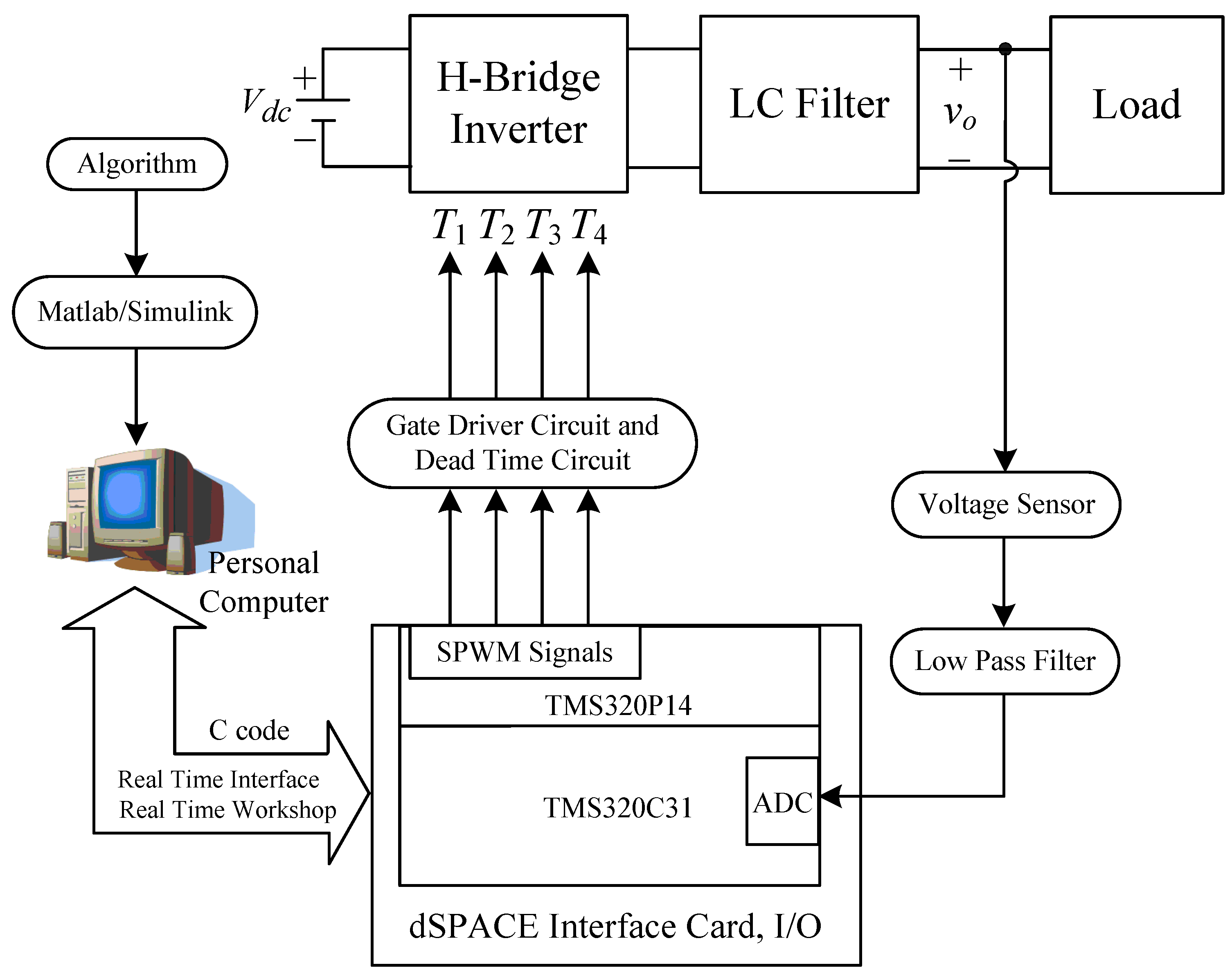
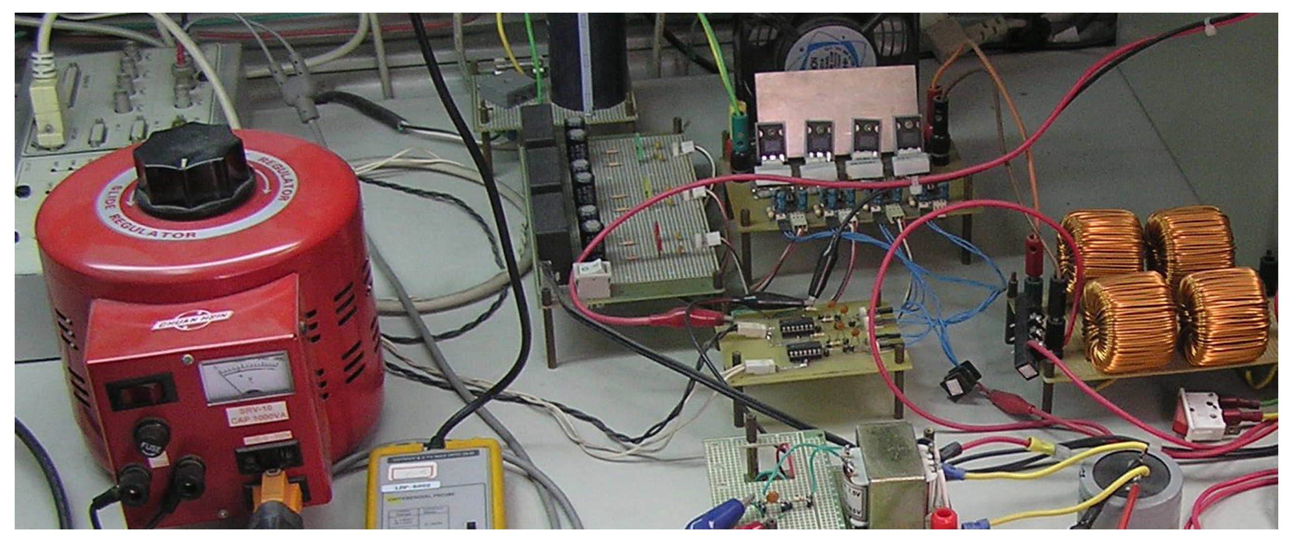
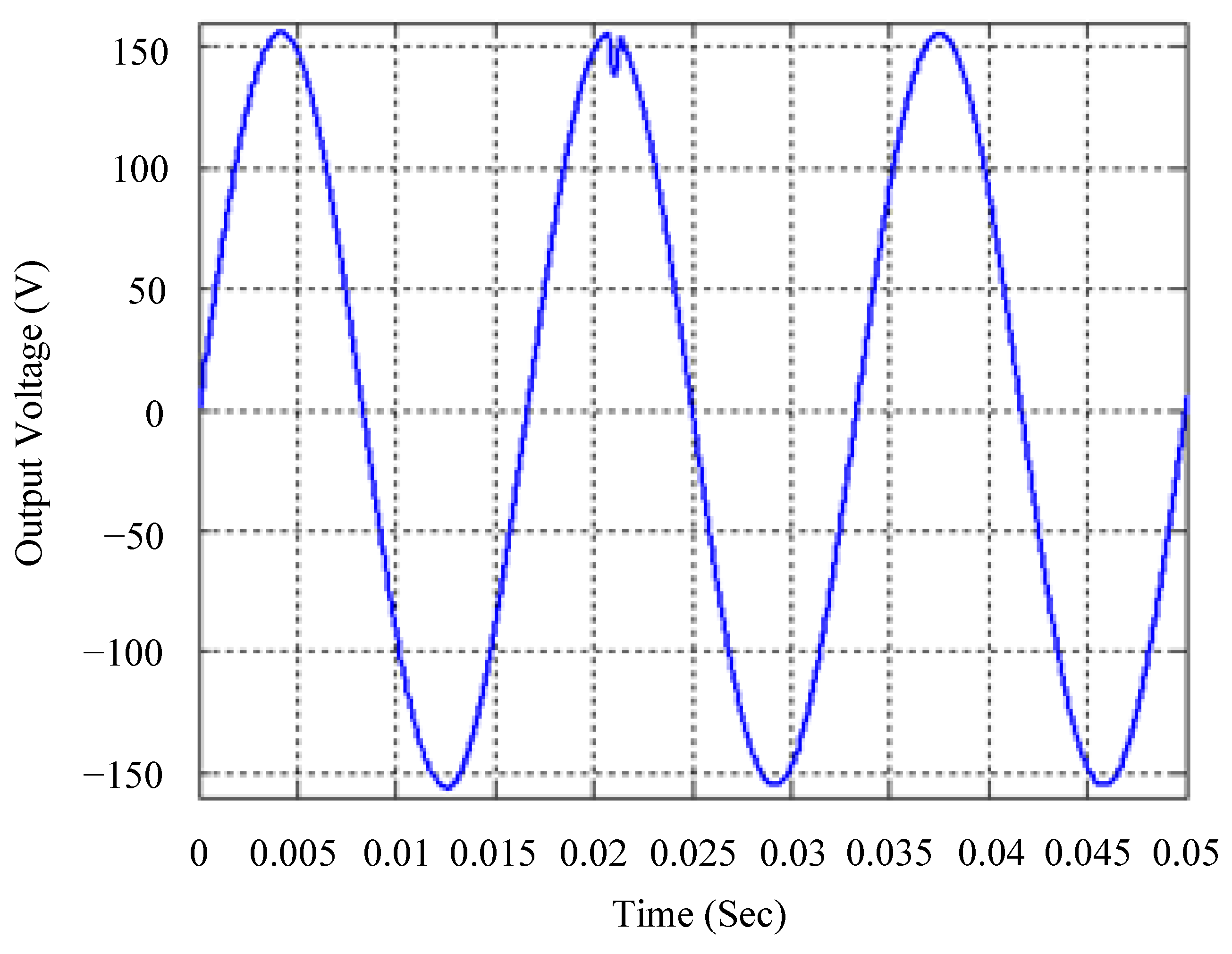
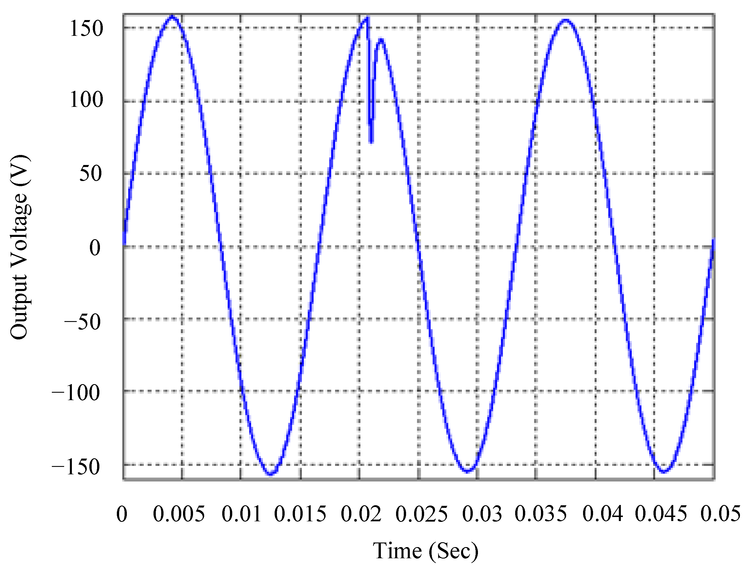
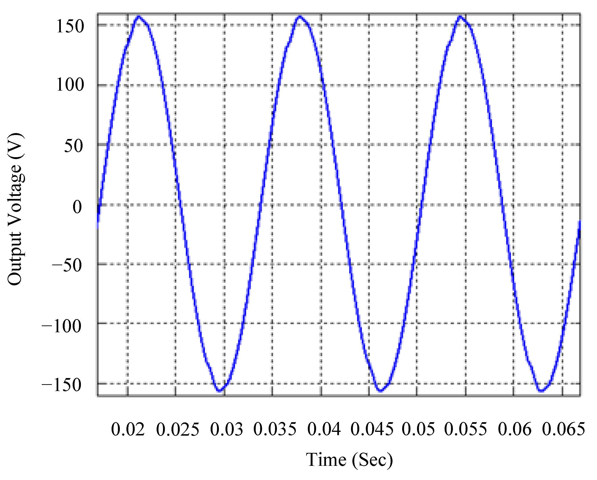
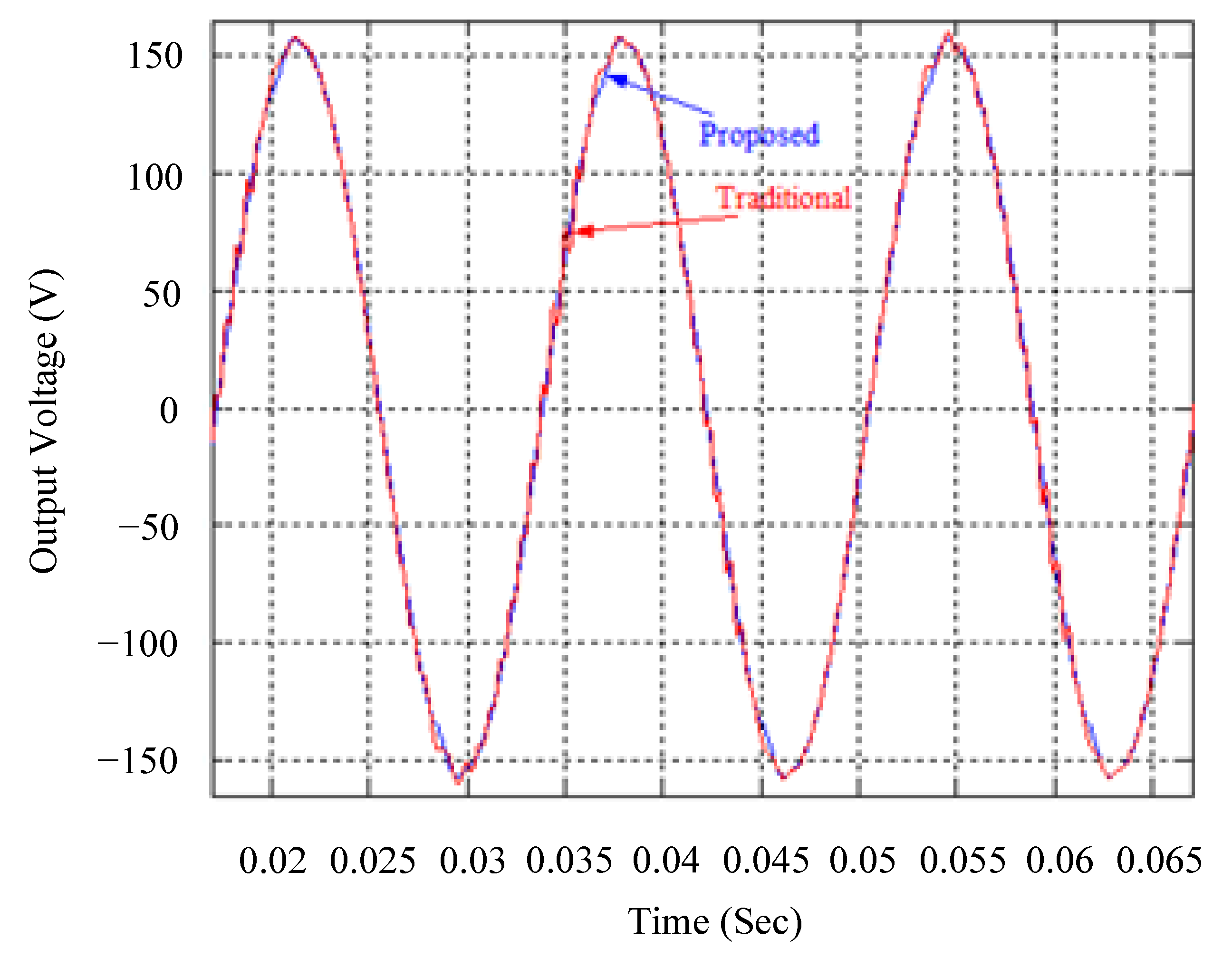
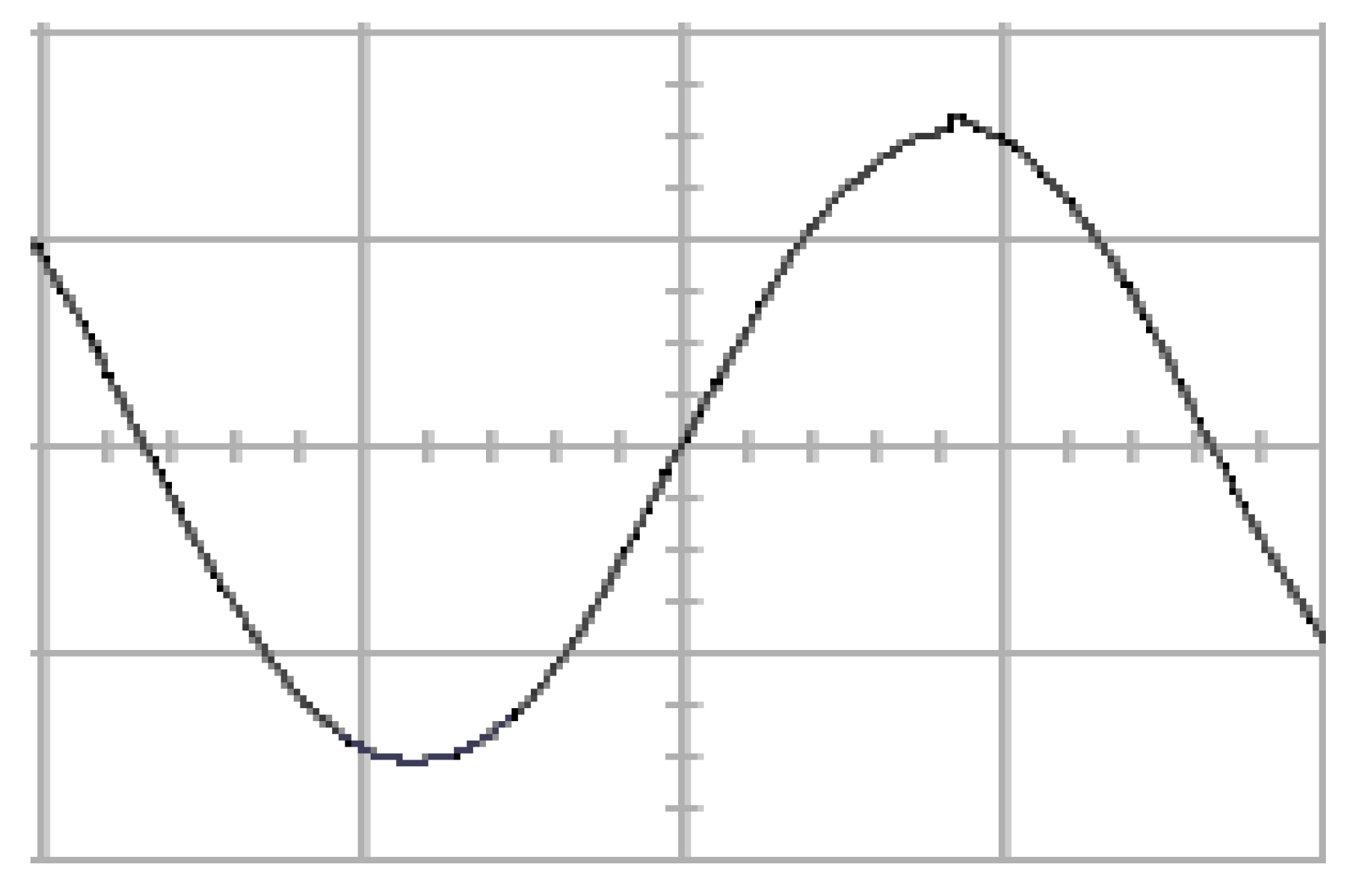
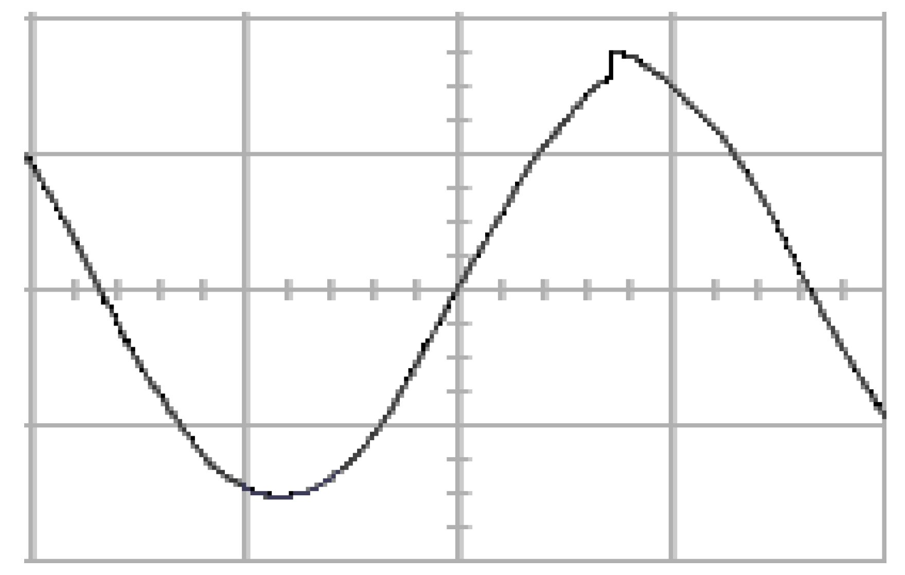
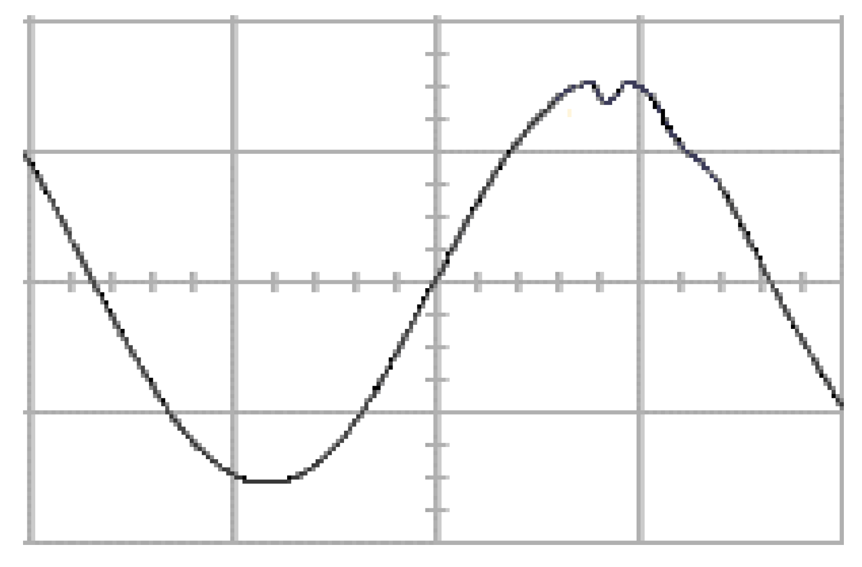
4. Simulated and Experimental Results

An H-bridge inverter with LC filter output has the parameters displayed in

Table 1. Parameters of the H-bridge inverter with LC filter output.

Parameters	Values
DC-link voltage ($V_{dc}$)	200 V
AC output voltage ($v_o$)	110 Vrms
Frequency of AC output-voltage	60 Hz
Filter inductor ($L$)	0.5 mH
Filter capacitor ($C$)	20 μF
Resistive load ($R_L$)	12 ohm
Switching frequency	25 kHz

. Simulation and experimental findings from this work were used to check the solvability of the proposed state-feedback control strategy. The MATLAB (version 6.1, MathWorks Inc., Natick, MA, USA)/Simulink (version 4.1, MathWorks Inc., Natick, MA, USA) software was employed to simulate the H-bridge inverter with LC filter output, which is operated with the proposed state-feedback control strategy as well as the traditional FTSMC. On the other hand, a dSPACE (dSPACE GmbH, Paderborn, Germany) digital signal processor (DSP) board implemented the H-bridge inverter with LC filter output. First, it is necessary to design the proposed state-feedback control strategy as well as the pulse width modulation (PWM) blocks in the MATLAB/Simulink environment. Then, the proposed control algorithm is automatically converted from Simulink diagrams to C codes, which can be implemented on the dSPACE real-time hardware. Figure 2 shows the overall control block diagram using the proposed state-feedback control strategy. The block diagram of the experimental setup and experimental hardware setup are displayed in Figure 3 and Figure 4, respectively.

The waveform of the proposed state-feedback control strategy applied to the H-bridge inverter with LC filter output is simulated in Figure 5 when there is a step-load change from full load to no load. The voltage swell occurs only slightly, and the waveform shows a sinusoidal form with nearly no oscillations. Figure 6 demonstrates the simulated voltage waveform of an H-bridge inverter with LC filter output based on the traditional FTSMC performed in the similar circumstance. The output voltage has a great voltage swell with poor transient response, even though the waveform also barely oscillates. Figure 7 compares the simulated output voltage difference between proposed state-feedback control strategy and traditional FTSMC for step-load change from full load to no load. It is obvious that the voltage swell of the traditional FTSMC exceeds 10% of the normal value, while that of the proposed state-feedback control strategy is very small, which approaches the normal value. Figure 8 and Figure 9, respectively, depict the simulated voltage waves of the proposed state-feedback control strategy as well as the traditional FTSMC during the step-load change from no load to full load. The traditional FTSMC fails to strike the sliding surface correctly, which causes chattering along with steady-state errors occurring within the short-term testing environment with such a large step-load changing behavior. The proposed state-feedback control strategy by the improved grey prediction ability can minimize the chattering as well as the steady-state error because it reacts promptly to the sliding surface, after which it accelerates the convergence to the equalization point. The output voltage with the proposed state-feedback control strategy recovers from a tiny voltage dip at approximately 16.45 V to the default voltage, whereas the output voltage with the traditional FTSMC returns to the default voltage after a drastic voltage dip of 84.79 V. The difference in the simulated output voltage for the proposed state-feedback control strategy and the traditional FTSMC at a step-load change from no load to full load is comparatively depicted in Figure 10. The voltage drop of the traditional FTSMC has about five times that of the state-feedback control strategy, presenting a quite poor transient response. With the aim of considering the performance characteristics of the proposed H-bridge inverter with LC filter output subjected to critically nonlinear loading such as a fully wave diode bridging rectifier incorporating an electrolytic capacitor along with a resistance load, the simulated output voltage waveform is given in Figure 11. There is a sine wave output voltage with fine robust steady-state preciseness, which was found to have less voltage THD of 0.17%. Nevertheless, given the same loading, the simulated waveform obtained from the traditional FTSMC is depicted in the Figure 12; the output voltage is up to 12.76%, showing a highly distorted sine wave. Figure 13 provides a comparison of the difference in the simulated output voltage at nonlinear rectifier load for the proposed state-feedback control strategy and the traditional FTSMC. Unlike the high-quality AC sine wave created by the proposed state-feedback control strategy, the traditional FTSMC causes oscillation and distortion in the output voltage, which occurs throughout the sine wave trajectory. The experimental waveforms of the output voltage generated by the H-bridge inverter with an LC filter output using the proposed state-feedback control strategy as well as the traditional FTSMC at step-load change from full load to no load are, respectively, shown in Figure 14 and Figure 15. The proposed state-feedback control strategy shows that the output voltage immediately reaches to the required AC voltage waveform after a minor voltage surge. However, the output voltage with the traditional FTSMC exhibits unsatisfactory transient behavior because of the occurrence of severe voltage swell. Figure 16 reveals the experiment output voltage in the H-bridge inverter with LC filter output based on the proposed state-feedback control strategy upon no load to full load-step transient changing. It can be recognized that the transient returns from a minor voltage dip fast, and an exact sinusoidal voltage waveform persists past the transient. The experiment output voltage waveform of the H-bridge inverter with LC filter output at the same testing condition for the traditional FTSMC is represented in Figure 17, where the big voltage dip along with the long restoration time can be seen. After a voltage dip of 17.76 V, the output voltage with the proposed state-feedback control strategy meets the demanding level because of the corrective mechanism of the improved grey prediction. Instead, following an 85.81 V voltage dip, the output voltage employing the traditional FTSMC was found to suffer from a bad oscillation tracking reaction near the firing angle. The performance of the H-bridge inverter with LC filter output subjected to grossly nonlinear rectified loads must be checked. Figure 18 and Figure 19 contain the experiment output voltage waveforms of the proposed state-feedback control strategy as well as those of the traditional FTSMC, separately. The traditional FTSMC H-bridge inverter with LC filter output has a warped output waveform with an oscillating sine wave voltage. The THD of the voltage is up to 14.48%, fairly poor steady-state behavior in conjunction with the lack of robustness. The output voltage of the proposed H-bridge inverter with LC filter output yields stable AC power with nearly distortion-free response (THD of 0.21%). There is no waveform oscillation caused by the nonlinear load condition, resulting in remarkably robust steady-state output characteristics.

Table 2. Simulated AC output voltage for voltage swell, voltage dip, and THD.

Proposed State-Feedback Control Strategy
Simulations	Step-load change (full load to no load)	Step-load change (no load to full load)	Rectified loading
	Voltage swell	Voltage dip	THD
	4.45 V	16.45 V	0.17%
Traditional FTSMC
Simulations	Step-load change (full load to no load)	Step-load change (no load to full load)	Rectified loading
	Voltage swell	Voltage dip	THD
	18.98 V	84.79 V	12.76%

as well as

Table 3. Experimental AC output voltage for voltage swell, voltage dip, and THD.

Proposed State-Feedback Control Strategy
Experiments	Step-load change (full load to no load)	Step-load change (no load to full load)	Rectified loading
	Voltage swell	Voltage dip	THD
	4.94 V	17.76 V	0.21%
Traditional FTSMC
Experiments	Step-load change (full load to no load)	Step-load change (no load to full load)	Rectified loading
	Voltage swell	Voltage dip	THD
	19.43 V	85.81 V	14.48%

give comparisons in terms of voltage swells, voltage dips, and THD. It is well verified from the simulation and experimental findings that the proposed state-feedback control strategy delivers slight voltage swell, less voltage dip, reduced THD, better steady-state accuracy, and more rapid convergence in all the tested scenarios. More precisely, IEEE (Institute of Electrical and Electronics Engineers) Standard 519-2014 [56] suggests that the maximum voltage total harmonic distortion target should be less than 8% for systems operating at a minimum voltage of 1 kV or less. Similarly, based on the IEC (International Electrotechnical Commission) standard, the IEC Standard 61000-2-2 [57] sets a level of compatibility margins in transmission of signals for public low-voltage supply systems, which also limits the total harmonic voltage distortion to 8%. The THD of the proposed H-bridge inverter with LC filter output is much lower than eight percent based on the IEEE Standard 519-2014 and IEC Standard 61000-2-2. Additionally, in terms of voltage drop and swell, IEEE Standard 1159-2019 [58] defines voltage drop between 10% and 90% of the nominal voltage, and the measured value is the root mean square (RMS) value of voltage at the power frequency during a period of one-half cycle to one minute; voltage swell is defined as a voltage RMS increase above 1.1 pu for a period of one-half cycle to one minute. In both the simulation and experimental results, the RMS value of voltage drop for the proposed state-feedback control strategy indicates about 12 V, which is in compliance with the limit of the IEEE Standard 1159-2019. But, the RMS value of voltage drop for the traditional FTSMC is approximately 60 V, thus exceeding the typical permissible value (the voltage is dropped to 70% of its standard value). For the proposed state-feedback control strategy, the RMS value of voltage swell is about 3 V, without over 10% of the nominal value, whereas a voltage swell of approximately 14 V RMS value for the traditional FTSMC exceeds the requirement of the IEEE Standard 1159-2019. The voltage dip in the IEC Standard 61000-4-30 [59] is defined as a reduction of the RMS voltage from one percent to ninety percent of the rated value for a period of 10 ms to 1 min; voltage swell indicates an instantaneous increase of ten percent or higher in RMS voltage for a duration of one-half cycle to one minute. The above-mentioned RMS values in voltage dip and swell for the proposed state-feedback control strategy also meet the specification of IEC Standard 61000-4-30, while vice versa for the traditional FTSMC. As a result, the voltage dip and swell of the proposed H-bridge inverter with LC filter output satisfy the limitations of both IEEE Standard 1159-2019 and IEC Standard 61000-4-30, presenting a satisfactory transient behavior.

5. Discussion and Analysis

The simulation and experimental findings of the H-bridge inverter with LC filter output meet the performance requirements of total harmonic distortion percentage and voltage sag. These can be attributed to the proposed state-feedback control strategy, but the design of the LC filter is another important consideration. Its design can be carried out according to the suggestions in past references. In order to downsize the size of the filter, it was decided to use a higher switching frequency, which is typically in the range of 20 kHz to 40 kHz for metal-oxide-semiconductor field-effect transistor switches. Next, a coefficient relative to the LC filter cutoff frequency needs to be regarded. A smaller value of this coefficient implies more attenuation and reduced enhancement at the switching and base frequencies; the smallest value of this coefficient can be reached, while a modulation value of 0.95 or less is preferred. It is also important to include a factor that correlates with the switching frequency and inductor ripple current, which should ideally be in the range of 20% to 40%. With these suggested factors in mind, the L and C settings can be assessed.

An additional interesting aspect is the sliding mode control in conjunction with depth enhancement learning for smoothing the control signal, which in turn helps to limit chattering as well as to boost the robustness of the control system [60,61,62,63,64]. A sliding mode control with model-free reinforcement learning was suggested to deliver the inverter voltage as the control operation of a hybrid static synchronous compensator for compensating the reactive power as well as harmonic from the loading. The presented approach exhibits good calculation effectiveness, high steady-state precision, quick reaction time, as well as better robustness [60]. With the objective of attaining the optimum agreement, a suggested approach examined decentralized control protocol design from undefined nonlinear multi-agent systems. The salient aspects of the development approach consist of decentralized sliding-mode control design as well as an interface platform for sliding-mode control and reinforcement learning. It yielded an achievement of success in learning a composite decentralized control protocol for a multi-agent system [61]. A new sliding mode tracking control law composed of an optimized tracking controller as well as an attack compensator was put forward to warrant the tracking behavior of a dual-time-scale system subjected to actuator attacks. This algorithm developed for the sliding mode tracking control law was realized by means of a reinforcement learning technique employing both slow as well as rapid sampling data [62]. The sliding mode control design approach was introduced for nonlinear systems at partial unknown dynamics through the integration of data-driven as well as model-based methodologies. It engineers sliding mode control for a nominal model as a nonlinear system and creates the necessary track for a partial known state of the nonlinear system exploiting the current model’s feedback state trajectory. The depth-strategy gradient algorithm handles the unexpected component of the system dynamics as well as tunes the sliding-mode control output towards the desirable state behavior [63]. An improved nominal model-based sliding mode controller allows fully exploiting the measurement data from the math modeling as well as the practical system to raise the following precision of vibration balancing location. An actor-critic-based reinforcement learning controller acquires a little backward compensating torque via the use of top flexible oscillation signals as well as the prioritized experienced recall law. It is stacked with the output of the nominal model-based sliding mode controller, in order to inhibit tip oscillation as well as to boost the localization precision of the hybrid structure flexible robot [64]. There are also some recommended recent publications focusing on the application of sliding mode control in power converters. Their research results demonstrate quite good dynamic and steady-state performance of the inverters that is worthy of reference for related researchers [65,66,67].

More recent publishing on grey prediction has enhanced the forecasting process through a grey polynomial model. It is a very helpful issue for the forecasting of systems loaded with unpredictability [68,69,70,71,72]. It is still necessary to conduct further studies on the selection of polynomials or polynomial coefficients for the grey polynomial model. After introducing tuned background coefficients in the grey polynomial model, then the suggested algorithmic framework for polynomial order picking, searching of background coefficients, as well as estimating of parameters was successfully proposed [68]. A novel time-delay polynomial grey prediction model had fractional order accumulation for forecasting in small samples. The new model took into account non-homogeneous terms, where the inside-sample modelling captures the prioritization of new messages in a superior manner [69]. A new grey prediction model incorporating a quadratic polynomial entry was also developed. By using the gray modeling technology as well as math tools, the time response function of the new model as well as the analysis expressing of the restored values were drawn up. The findings reveal that the new model offers greater predictive precision for COVID-19 [70]. The fractional accumulation power generation operator as well as the time power item were realized in the discrete grey polynomial model. The quantum genetic algorithm identifies the emerging coefficients with the aim of further augmenting the forecasting precision. The presented model reaches the optimum forecasting property in terms of its low average absolute percentage error for natural gas consideration, power generation, as well as for the elderly population [71]. An optimizing polynomial grey model for fractional overhead power entries was suggested. The coefficients of the polynomial grey role amount are gained in a way that seeks to minimalize the forecasting error, which reports the usage of linear population sizing degradation as well as alternative contemporary optimizers in making optimal use of the whitening equations. The proposed method was applied to forecast clearing prices in the market, where the findings indicated that the presented modelling gives a substantially higher fitting efficacy [72].

In future research, the proposed state-feedback control strategy has the feasibility of implementation in actual power systems. However, there are some potential challenges, like the fact that both the inverter and the grid have to be synchronized (i.e., the same frequency, phase, and magnitude); this can be ensured by considering a phase-locked loop (PLL) algorithm. Also, for improving the quality of grid current, a grid-connected inverter can use an inductor-capacitor-inductor (LCL) filter with better ability in reducing harmonics, but the peak resonance problem may occur in the system, and this can be mitigated through the passive/active damping method.

6. Conclusions

In this paper, a fast finite-time sliding mode control with compensation of grey prediction model in a center-approximation-based method was found to have high efficiency as well as computational ease for the H-bridge inverter with LC filter output, generating sound sine-wave response behavior. Despite the fact that finite-time sliding mode control enjoys a time-limited state convergence in comparison to regular SMC, the fast finite-time sliding mode control responding trajectory converges to the balancing moment sooner than that of finite-time sliding mode control. Furthermore, while FTSMC occasionally faces the challenge of singularities, FFTSMC ameliorates this issue while being immune to irregularities, giving it an attractive advantage amongst the numerous other types of SMC. Regarding the bounds of exaggerated or insufficiently assessed state uncertainties in the system, chattering or steady-state errors emerge in the FFTSMC, elevating the output voltage harmonics of the H-bridge inverter with LC filter output. The grey prediction adopted in this paper retains the benefit of typical grey prediction, needing just a certain restricted number of data for modeling purposes; in particular, it involves the use of a centered approximation method, giving a higher precision estimation of the undetermined state’s behavior, thus abolishing chattering as well as steady-state errors. Both simulated as well as experimentally conducted findings of closed-loop managed H-bridge inverter with LC filter output were applied to justify the proposed state-feedback control strategy. It was found that the dynamic and steady-state characteristics of the H-bridge inverter with LC filter output lead to a remarkably fast reaction as well as considerably low total harmonic distortion especially among heavily step-load changing, dramatically varied parameter values of the filter as well as nonlinear loading. Furthermore, the proposed H-bridge inverter with LC filter output can be used for various practical applications in industry, such as uninterruptible power supplies, induction heating, induction motor drives, and renewable energy systems; this is because the proposed state-feedback control strategy exhibits the advantages of faster finite-time state convergence, chattering mitigation, and the reduction of steady-state errors.

References

1. Sundaramoorthy, S.; Sundaram, S.S.M.; Sakthivel, S.S. Cascaded H-Bridge Inverter Control for Grid Connected DC Power Source: Design and Analysis of Cascaded H-Bridge Multilevel Inverter with PWM Techniques and Controllers; LAP LAMBERT Academic Publishing: London, UK, 2019. [Google Scholar]
2. Aboadla, E.H.; Khan, S.; Abdul Kadir, K.; Md Yusof, Z.; Habaebi, M.H.; Habib, S.; Islam, M.; Hasan, M.K.; Hossain, E. Suppressing Voltage Spikes of MOSFET in H-Bridge Inverter Circuit. Electronics 2021, 10, 390. [Google Scholar] [CrossRef]
3. Zammit, D.; Staines, C.S.; Apap, M. Compensation techniques for non-linearities in H-bridge inverters. J. Electr. Syst. Inf. Technol. 2016, 3, 361–376. [Google Scholar] [CrossRef]
4. Smith, G. Introduction to Modern Power Electronics; Larsen and Keller Education: New York, NY, USA, 2017. [Google Scholar]
5. Rozanov, Y.; Ryvkin, S.E.; Chaplygin, E.; Voronin, P. Power Electronics Basics Operating Principles, Design, Formulas, and Applications; CRC Press: Boca Raton, FL, USA, 2016. [Google Scholar]
6. Kumar, V.; Behera, R.K.; Joshi, D.; Bansal, R. Power Electronics, Drives, and Advanced Applications; CRC Press: Boca Raton, FL, USA, 2020. [Google Scholar]
7. Mohan, A.; Jos, B.M.; Sreekumar, S.; Hima, T. Implementation of Constant Switching Frequency Hysteresis based Current Control of Solar PV Inverter. In Proceedings of the 2023 8th International Conference on Communication and Electronics Systems (ICCES), Coimbatore, India, 1–3 June 2023; pp. 40–44. [Google Scholar]
8. Gulbudak, O.; Gokdag, M. FPGA-Based Hysteresis Current Control for Induction Motor fed by a Voltage-Source Inverter. In Proceedings of the 2023 5th Global Power, Energy and Communication Conference (GPECOM), Nevsehir, Turkiye, 14–16 June 2023; pp. 147–152. [Google Scholar]
9. Yang, Y.; Yang, Y.; He, L.Q.; Fan, M.D.; Xiao, Y.; Chen, R.; Xie, M.X.; Zhang, X.A.; Zhang, L.J.; Rodriguez, J. A Novel Cascaded Repetitive Controller of an LC-Filtered H6 Voltage-Source Inverter. IEEE J. Emerg. Sel. Top. Power Electron. 2023, 11, 556–566. [Google Scholar] [CrossRef]
10. Ye, Y.; Zhang, B.; Zhou, K.; Wang, D.; Wang, Y. High-Performance Cascade-Type Repetitive Controller for CVCF PWM Inverter: Analysis and Design. IET Electr. Power Appl. 2007, 1, 112–118. [Google Scholar] [CrossRef]
11. Chen, T.F.; Dutta, O.; Ramasubramanian, D.; Farantatos, E. An LQR-based Robust Voltage Controller for Grid Forming Inverters during Blackstart. In Proceedings of the 2021 IEEE PES Innovative Smart Grid Technologies–Asia (ISGT Asia), Brisbane, Australia, 5–8 December 2021; pp. 1–5. [Google Scholar]
12. Zhou, H.; Liu, J.; Zhang, P.; Ma, M.; Fang, Z.; Zeng, J. Linear Quadratic Regulator Optimized Feedback Control Method for Resonant Inverter Power Supply in High Frequency AC Power Distribution of Electric Vehicle. In Proceedings of the 2022 Tsinghua–IET Electrical Engineering Academic Forum, Beijing, China and Online, 28–29 May 2022; pp. 1–7. [Google Scholar]
13. Blachuta, M.; Rymarski, Z.; Bieda, R.; Bernacki, K.; Grygiel, R. Design, Modeling and Simulation of PID Control for DC/AC Inverters. In Proceedings of the 2019 24th International Conference on Methods and Models in Automation and Robotics (MMAR), Miedzyzdroje, Poland, 26–29 August 2019; pp. 428–433. [Google Scholar]
14. Ucchas, M.T.W.; Nuhas, M.M.; Toufiquzzaman, M.; Mahmud, A.J.; Islam, M.F. Performance and Comparative Analysis of PI and PID Controller-based Single Phase PWM Inverter Using MATLAB Simulink for Variable Voltage. In Proceedings of the 2022 Second International Conference on Advances in Electrical, Computing, Communication and Sustainable Technologies (ICAECT), Bhilai, India, 21–22 April 2022; pp. 1–6. [Google Scholar]
15. Kumar, M.; Sen, S.; Kumar, S. A Robust Performance Analysis of a Solar PV-battery based Islanded Microgrid Inverter output Voltage Control using Dual-loop PID Controller. In Proceedings of the 2022 IEEE IAS Global Conference on Emerging Technologies (GlobConET), Arad, Romania, 20–22 May 2022; pp. 1–6. [Google Scholar]
16. He, J.S.; Zhang, X. Comparison of the Back-Stepping and PID Control of the Three-Phase Inverter with Fully Consideration of Implementation Cost and Performance. Chin. J. Electr. Eng. 2018, 4, 82–89. [Google Scholar]
17. Oliveira, T.R.; Fridman, L.; Hsu, L. Sliding-Mode Control and Variable-Structure Systems; Springer: Cham, Switzerland, 2023. [Google Scholar]
18. Edwards, C.; Spurgeon, S. Sliding Mode Control Theory and Applications; CRC Press: Boca Raton, FL, USA, 1998. [Google Scholar]
19. Vaidyanathan, S.; Lien, C.H. Applications of Sliding Mode Control in Science and Engineering; Springer: New York, NY, USA, 2017. [Google Scholar]
20. Özkara, Ö.; Ortatepe, Z.; Karaarslan, A. Implementation of Sliding Mode Control Method for Switched-Inductor Quasi-Z-Source Inverter. In Proceedings of the 2022 Global Energy Conference (GEC), Batman, Turkey, 26–29 October 2022; pp. 179–184. [Google Scholar]
21. Anjum, W.; Husain, A.R.; Abdul, A.J.; Abbasi, M.A.; Alqaraghuli, H. Continuous Dynamic Sliding Mode Control Strategy of PWM Based Voltage Source Inverter Under Load Variations. PLoS ONE 2020, 15, e0228636. [Google Scholar] [CrossRef] [PubMed]
22. Rajakumar, V.; Anbukumar, K.; Selwynraj, A.I. Sliding Mode Controller-Based Voltage Source Inverter for Power Quality Improvement in Microgrid. IET Renew. Power Gener. 2020, 14, 1860–1872. [Google Scholar] [CrossRef]
23. Chaturvedi, S.; Fulwani, D. Integral Sliding Mode Control for Uncertainty Mitigation in Switched Boost Inverters. In Proceedings of the 2020 IEEE 9th Power India International Conference (PIICON), Sonepat, India, 28 February–1 March 2020; pp. 1–6. [Google Scholar]
24. Pho, B.B.; Tran, T.M.; Nguyen, M.L.; Hoang, P.V. Discrete-Time Quasi Sliding Mode Control of Single-phase T-type Inverters for Residential PV Applications. In Proceedings of the 2020 International Conference on Advanced Mechatronic Systems (ICAMechS), Hanoi, Vietnam, 10–13 December 2020; pp. 1–6. [Google Scholar]
25. Wu, L.G.; Liu, J.X.; Vazquez, S.; Mazumder, S.K. Sliding Mode Control in Power Converters and Drives: A Review. IEEE/CAA J. Autom. Sin. 2022, 9, 392–406. [Google Scholar] [CrossRef]
26. Chen, M.H. Input-Output Finite-Time Sliding Mode Control of Discrete Time-Varying Systems Under an Adaptive Event-Triggered Mechanism. IEEE Access 2023, 11, 3555–3563. [Google Scholar] [CrossRef]
27. Dhar, S.; Dash, P.K. A New Backstepping Finite Time Sliding Mode Control of Grid Connected PV System Using Multivariable Dynamic VSC Model. Int. J. Electr. Power Energy Syst. 2016, 82, 314–330. [Google Scholar] [CrossRef]
28. Sun, C.B.; Wang, S.B.; Yu, H.S. Finite-Time Sliding Mode Control Based on Unknown System Dynamics Estimator for Nonlinear Robotic Systems. IEEE Trans. Circuits Syst. II Express Briefs 2023, 70, 2535–2539. [Google Scholar] [CrossRef]
29. Wongvanich, N.; Roongmuanpha, N.; Tangsrirat, W. Finite-Time Integral Backstepping Nonsingular Terminal Sliding Mode Control to Synchronize a New Six-Term Chaotic System and Its Circuit Implementation. IEEE Access 2023, 11, 22233–22249. [Google Scholar] [CrossRef]
30. Hu, M.Y.; Ahn, H.; You, K.H. Finite-Time Rapid Global Sliding-Mode Control for Quadrotor Trajectory Tracking. IEEE Access 2023, 11, 22364–22375. [Google Scholar] [CrossRef]
31. Dong, H.L.; Yang, X.B.; Gao, H.J.; Yu, X.H. Practical Terminal Sliding-Mode Control and Its Applications in Servo Systems. IEEE Trans. Ind. Electron. 2023, 70, 752–761. [Google Scholar] [CrossRef]
32. Narayan, J.; Abbas, M.; Dwivedy, S.K. Robust Non-Singular Fast Terminal Sliding Mode Gait Tracking Control of a Pediatric Exoskeleton. In Proceedings of the 2023 5th International Conference on Bio-Engineering for Smart Technologies (BioSMART), Paris, France, 7–9 June 2023; pp. 1–4. [Google Scholar]
33. Kim, Y.J.; Ahn, H.K.; Hu, M.Y.; You, K.H. Improved Non-Singular Fast Terminal Sliding Mode Control for SPMSM Speed Regulation. IEEE Access 2023, 11, 65924–65933. [Google Scholar] [CrossRef]
34. Zhang, T.; Jiao, X.H.; Zhang, Y.H. EID-Based Finite-Time Nonsingular Fast Terminal Sliding Mode Control of Autonomous Farming Vehicle. In Proceedings of the 2022 13th Asian Control Conference (ASCC), Jeju, Republic of Korea, 4–7 May 2022; pp. 579–584. [Google Scholar]
35. Yang, W.L.; Fan, Y.Q.; Xu, D.Z.; Pan, T.L.; Dong, Y. A Stochastic Configuration Networks-Based Nonsingular Fast Terminal Sliding Mode Control Approach for Indirect Matrix Converter-Driven Permanent Magnet Linear Synchronous Motors. Ind. Artif. Intell. 2023, 1, 6. [Google Scholar] [CrossRef]
36. Lian, S.K.; Meng, W.; Shao, K.; Zheng, J.C.; Zhu, S.Q.; Li, H.Y. Full Attitude Control of a Quadrotor Using Fast Nonsingular Terminal Sliding Mode with Angular Velocity Planning. IEEE Trans. Ind. Electron. 2023, 70, 3975–3984. [Google Scholar] [CrossRef]
37. Olivas-Martínez, G.; Castañeda, H. Adaptive Single-Gain Non-Singular Fast Terminal Sliding Mode Control for a Quad-rotor UAV Against Wind Perturbations. In Proceedings of the 2023 International Conference on Unmanned Aircraft Systems (ICUAS), Warsaw, Poland, 6–9 June 2023; pp. 1148–1154. [Google Scholar]
38. Nie, J.; Hao, L.C.; Zhang, G.H.; Li, Q.; Zhang, X.Y. Nonsingular Fast Terminal Sliding Mode Control of Manipulator Trajectory Tracking Based on Adaptive Finite-Time Disturbance Observer. In Proceedings of the 2023 IEEE International Conference on Mechatronics and Automation (ICMA), Harbin, Heilongjiang, China, 6–9 August 2023; pp. 1149–1154. [Google Scholar]
39. Mobayen, S.; Baleanu, D.; Tchier, F. Second-Order Fast Terminal Sliding Mode Control Design Based on LMI for a Class of Non-Linear Uncertain Systems and its Application to Chaotic Systems. J. Vib. Control. 2017, 23, 2912–2925. [Google Scholar] [CrossRef]
40. Yang, Y.J.; Liu, S.F. Emerging Studies and Applications of Grey Systems; Springer: Singapore, 2023. [Google Scholar]
41. Liu, S.; Yang, Y.; Forrest, J. Grey Data Analysis: Methods, Models and Applications; Springer: Singapore, 2016. [Google Scholar]
42. Deng, J.L. Introduction to Grey System Theory. J. Grey Syst. 1989, 1, 1–24. [Google Scholar]
43. Liu, S.F.; Lin, Y. Grey Information: Theory and Practical Applications; Springer: London, UK, 2006. [Google Scholar]
44. Xie, N.M.; Liu, S.F. Discrete Grey Forecasting Model and Its Optimization. Appl. Math. Model. 2009, 33, 1173–1186. [Google Scholar] [CrossRef]
45. Zhang, Y.P.; Li, M.S. Grey System Forecasting Based on MATLAB and Its Example Application. In Proceedings of the 2010 2nd IEEE International Conference on Information Management and Engineering, Chengdu, China, 16–18 April 2010; pp. 48–52. [Google Scholar]
46. Shen, Q.Q.; Shi, Q.; Tang, T.P.; Yao, L.Q. A Novel Weighted Fractional GM(1,1) Model and Its Applications. Complexity 2020, 2020, 6570683. [Google Scholar] [CrossRef]
47. Bilgil, H. New Grey Forecasting Model with Its Application and Computer Code. AIMS Math. 2020, 6, 1497–1514. [Google Scholar] [CrossRef]
48. Li, X.Z.; Kong, J.M.; Wang, C.H. Application of Center Approach Grey GM(1,1) Model to Prediction of Landslide Deformation with a Case Study. J. Eng. Geol. 2007, 15, 673–676. [Google Scholar]
49. Song, Z.; Tong, X.; Xiao, X. Center Approach Grey GM (1, 1) Model. Syst. Eng.-Theory Pract. 2001, 21, 110–113. [Google Scholar]
50. Qiu, L.; Zhou, M.; Wei, M.H. Center Approach Grey BP Neural Network Prediction Model for Years of Drought Occurrence in Xinzhou District of Wuhan City. In Proceedings of the 2011 5th International Conference on Bioinformatics and Biomedical Engineering, Wuhan, China, 10–12 May 2011; pp. 1–4. [Google Scholar]
51. Liu, M.; Zhao, L.D. An Improved GLP Model Base on Complete Center Approach GM(1,1) for Emergency Logistics Distribution. In Proceedings of the 2007 IEEE International Conference on Grey Systems and Intelligent Services, Nanjing, China, 18–20 November 2007; pp. 428–433. [Google Scholar]
52. Liu, F.; Wei, X.K.; Liu, Y.; Yin, X.X. Track Quality Prediction Based on Center Approach Markov-Grey GM(1,1) Model. In Proceedings of the 2014 IEEE International Conference on Information and Automation (ICIA), Hailar, China, 28–30 July 2014; pp. 81–86. [Google Scholar]
53. Cao, Y.Q.; Wang, Y.M.; Xia, H.W. Non-singular Terminal Sliding Mode Control of DC-DC Buck Converter with Fixed Frequency. In Proceedings of the 2016 35th Chinese Control Conference (CCC), Chengdu, China, 27–29 July 2016; pp. 3452–3456. [Google Scholar]
54. Gao, Z.Y.; Guo, G.; Zhang, B. Non-singular Terminal Sliding Mode Heading Control of Surface Vehicles. In Proceedings of the 2017 36th Chinese Control Conference (CCC), Dalian, China, 26–28 July 2017; pp. 634–638. [Google Scholar]
55. Lademakhi, N.Y.; Shiri, R.; Korayem, A.H. Superiority of Finite Time SDRE and Non-singular Terminal SMC Controller for n-DOF Manipulators. In Proceedings of the 6th RSI International Conference on Robotics and Mechatronics (IcRoM 2018), Tehran, Iran, 23–25 October 2018; pp. 315–321. [Google Scholar]
56. IEEE Standard 519-2014; IEEE 519 Recommended Practice and Requirements for Harmonic Control in Electric Power Systems. IEEE: New York, NY, USA, 2014.
57. IEC Standard 61000-2-2; Environment-Compatibility Levels for Low-Frequency Conducted Disturbances and Signalling in Public Low-Voltage Power Supply Systems. IEC: Geneva, Switzerland, 2002.
58. IEEE Standard 1159–2019; IEEE Recommended Practice for Monitoring Electric Power Quality. IEEE: New York, NY, USA, 2019.
59. IEC Standard 61000-4-30; Testing and Measurement Techniques-Power Quality Measurement Methods. IEC: Geneva, Switzerland, 2015.
60. Gong, C.; Sou, W.K.; Lam, C.S. Reinforcement Learning Based Sliding Mode Control for a Hybrid-STATCOM. IEEE Trans. Power Electron. 2023, 38, 6795–6800. [Google Scholar] [CrossRef]
61. Li, J.N.; Yuan, L.; Chai, T.Y.; Lewis, F.L. Consensus of Nonlinear Multiagent Systems with Uncertainties Using Reinforcement Learning Based Sliding Mode Control. IEEE Trans. Circuits Syst. I Regul. Pap. 2023, 70, 424–434. [Google Scholar] [CrossRef]
62. Zhang, Y.; Ma, L.; Yang, C.Y.; Dai, W. Reinforcement Learning-Based Sliding Mode Tracking Control for the Two-Time-Scale Systems: Dealing with Actuator Attacks. IEEE Trans. Circuits Syst. II Express Briefs 2022, 69, 3819–3823. [Google Scholar] [CrossRef]
63. Mosharafian, S.; Afzali, S.; Bao, Y.J.; Velni, J.M. A Deep Reinforcement Learning-based Sliding Mode Control Design for Partially-known Nonlinear Systems. In Proceedings of the 2022 European Control Conference (ECC), London, UK, 12–15 July 2022; pp. 2241–2246. [Google Scholar]
64. Long, T.; Li, E.; Hu, Y.Q.; Yang, L.; Fan, J.F.; Liang, Z.Z.; Guo, R. A Vibration Control Method for Hybrid-Structured Flexible Manipulator Based on Sliding Mode Control and Reinforcement Learning. IEEE Trans. Neural Netw. Learn. Syst. 2021, 32, 841–852. [Google Scholar] [CrossRef]
65. Shen, X.N.; Liu, J.X.; Liu, Z.; Gao, Y.B.; Leon, J.I.; Vazquez, S.; Wu, L.G.; Franquelo, L.G. Sliding Mode Control of Neutral-Point-Clamped Power Converters with Gain Adaptation. IEEE Trans. Power Electron. 2024, 1–13. [Google Scholar] [CrossRef]
66. Shen, X.N.; Wu, C.W.; Liu, Z.; Wang, Y.J.; Leon, J.I.; Liu, J.X.; Franquelo, L.G. Adaptive-Gain Second-Order Sliding-Mode Control of NPC Converters Via Super-Twisting Technique. IEEE Trans. Power Electron. 2023, 38, 15406–15418. [Google Scholar] [CrossRef]
67. Liu, J.X.; Shen, X.N.; Alcaide, A.M.; Yin, Y.F.; Leon, J.I.; Vazquez, S.; Wu, L.G.; Franquelo, L.G. Sliding Mode Control of Grid-Connected Neutral-Point-Clamped Converters Via High-Gain Observer. IEEE Trans. Ind. Electron. 2022, 69, 4010–4021. [Google Scholar] [CrossRef]
68. Wei, B.L.; Xie, N.M.; Hu, A. Optimal Solution for Novel Grey Polynomial Prediction Model. Appl. Math. Model. 2018, 62, 717–727. [Google Scholar] [CrossRef]
69. Chen, L.; Liu, Z.B.; Ma, N.N. Time-Delayed Polynomial Grey System Model with the Fractional Order Accumulation. Math. Probl. Eng. 2018, 2018, 3640625. [Google Scholar] [CrossRef]
70. Zhang, J.; Jiang, Z. A New Grey Quadratic Polynomial Model and Its Application in the COVID–19 in China. Sci. Rep. 2021, 11, 12588. [Google Scholar] [CrossRef] [PubMed]
71. Liu, C.; Wu, W.Z.; Xie, W. Study of the Generalized Discrete Grey Polynomial Model Based on the Quantum Genetic Algorithm. J. Supercomput. 2021, 77, 11288–11309. [Google Scholar] [CrossRef]
72. Saxena, A. Optimized Fractional Overhead Power Term Polynomial Grey Model (OFOPGM) for Market Clearing Price Prediction. Electr. Power Syst. Res. 2023, 214, 108800. [Google Scholar] [CrossRef]
Figure 1. General structure of an H-bridge inverter with LC filter output: (a) Circuit diagram. (b) Switching pulses.
Electronics 13 02118 g001
Figure 2. Block diagram using the proposed state-feedback control strategy in MATLAB/Simulink software environment.
Electronics 13 02118 g002
Figure 3. Block diagram of experimental setup.
Electronics 13 02118 g003
Figure 4. Experimental hardware setup.
Electronics 13 02118 g004
Figure 5. Simulated output voltage at step-load change (from full load to no load) with proposed state-feedback control strategy.
Electronics 13 02118 g005
Figure 6. Simulated output voltage at step-load change (from full load to no load) with traditional FTSMC.
Electronics 13 02118 g006
Figure 7. Simulated output voltage difference at step-load change (from full load to no load) between proposed state-feedback control strategy and traditional FTSMC.
Electronics 13 02118 g007
Figure 8. Simulated output voltage at step-load change (from no load to full load) with proposed state-feedback control strategy.
Electronics 13 02118 g008
Figure 9. Simulated output voltage at step-load change (from no load to full load) with traditional FTSMC).
Electronics 13 02118 g009
Figure 10. Simulated output voltage difference at step-load change (from no load to full load) between proposed state-feedback control strategy and traditional FTSMC.
Electronics 13 02118 g010
Figure 11. Simulated output voltage at rectified loading with proposed state-feedback control strategy.
Electronics 13 02118 g011
Figure 12. Simulated output voltage at rectified loading with traditional FTSMC.
Electronics 13 02118 g012
Figure 13. Simulated output voltage difference at rectified loading between proposed state-feedback control strategy and traditional FTSMC.
Electronics 13 02118 g013
Figure 14. Experimental output voltage at step-load change (from full load to no load) with proposed state-feedback control strategy (vertical: 100 V/div; horizontal: 5 ms/div).
Electronics 13 02118 g014
Figure 15. Experimental output voltage at step-load change (from full load to no load) with traditional FTSMC (vertical: 100 V/div; horizontal: 5 ms/div).
Electronics 13 02118 g015
Figure 16. Experimental output voltage at step-load change (from no load to full load) with proposed state-feedback control strategy (vertical: 100 V/div; horizontal: 5 ms/div).
Electronics 13 02118 g016
Figure 17. Experimental output voltage at step-load change (from no load to full load) with traditional FTSMC (vertical: 100 V/div; horizontal: 5 ms/div).
Electronics 13 02118 g017
Figure 18. Experimental output voltage at rectified loading with proposed state-feedback control strategy (vertical: 100 V/div; horizontal: 5 ms/div).
Electronics 13 02118 g018
Figure 19. Experimental output voltage at rectified loading with traditional FTSMC (vertical: 100 V/div; horizontal: 5 ms/div).
Electronics 13 02118 g019