A Bayesian Deep Unfolded Network for the Off-Grid Direction-of-Arrival Estimation via a Minimum Hole Array

Abstract

As an important research focus in radar detection and localization, direction-of-arrival (DOA) estimation has advanced significantly owing to deep learning techniques with powerful fitting and classifying abilities in recent years. However, deep learning inevitably requires substantial data to ensure learning and generalization abilities and lacks reasonable interpretability. Recently, a deep unfolding technique has attracted widespread concern due to the more explainable perspective and weaker data dependency. More importantly, it has been proven that deep unfolding enables convergence acceleration when applied to iterative algorithms. On this basis, we rigorously deduce an iterative sparse Bayesian learning (SBL) algorithm and construct a Bayesian deep unfolded network in a one-to-one correspondence. Moreover, the common but intractable off-grid errors, caused by grid mismatch, are directly considered in the signal model and computed in the iterative process. In addition, minimum hole array, little considered in deep unfolding, is adopted to further improve estimation performance owing to the maximized array degrees of freedom (DOFs). Extensive simulation results are presented to illustrate the superiority of the proposed method beyond other state-of-the-art methods.

1. Introduction

As an active research focus, direction-of-arrival (DOA) estimation has advanced significantly over the past four decades owing to the adopted subspace, compressed sensing, and deep learning that led to technology leaps [1,2,3]. In particular, deep learning is highly favored by researchers due to the powerful fitting and classifying abilities that play important roles in image and signal processing [4,5]. However, as a data-driven technique, deep learning requires abundant sampling data for training and empirically complicated network architectures for nonlinear fitting [6], while numerous data are not always easy to collect, and too deep and elaborate networks may lead to gradient explosion or vanishing. Additionally, the lack of explainable theory simultaneously leads to the limitation of application and development [7]. Hence, the pursuit of more explainable learning networks is becoming a research focus. Recently, deep unfolding has been proven to achieve them [8].

In contrast to empirical deep learning, deep unfolding, first developed for sparse coding [9], is rigorously based on iterative algorithms [10]. Specifically, deep unfolding enhances interpretability by constructing a network corresponding to the specific iterative steps of theoretically believable algorithms. Therefore, deep unfolding essentially belongs to a compromise between data-driven and model-based methods. On the one hand, deep unfolding is more explainable since the effect of every layer and each neuron explicitly originated from iterative algorithms. On the other hand, deep unfolding inherits the advantages of deep learning, i.e., excellent robustness to modeling errors and strong adaptability to complicated cases that model-based algorithms tend to be at a loss. More importantly, deep unfolding is able to improve convergence rates [11,12], though only LSTA-net [13] and ADMM-net [14] have been proven theoretically. In fact, deep unfolding still empirically shows desirable performance. In the DOA estimation field, a deep unfolded FOCUSS network is developed in [15] for on-grid and off-grid DOA estimation, resulting in low complexity and high estimation accuracy. Additionally, a deep Alternating Projection Network for gridless DOA estimation is proposed in [16], achieving super-resolution estimation. Moreover, ISTA is also adopted for deep unfolding [17,18] so that the proposed method can handle anti-jamming, array imperfections, and noise. In the channel estimation field, there are many works using deep unfolding to improve estimation performance. ISTA-based deep unfolded networks are developed for high running efficiency and excellent estimation performance [19,20], while the same operation is adopted for ADMM and AMP. Moreover, RIS and SSCA algorithms are introduced for constructing deep unfolded networks [21] so that the computation complexity and signaling overhead are decreased when compared with the original algorithms.

Overall, many works have adopted iterative algorithms converging slowly to improve convergence efficiency for DOA or channel estimation. Nonetheless, the developed deep unfolded networks are limited to their original algorithms. In other words, the original iterative algorithms dominate the main performance of the deep unfolded networks. Thus, it seems to be the best selection to apply excellent iterative algorithms to be unfolded. As we know, sparse Bayesian learning (SBL) [22,23] is an excellent probabilistic algorithm for linear regression. Unlike the above deterministic algorithms with explicit regularization constraints, SBL leverages prior distributions assigned to latent variables for regularization constraint, so the sparsity performance is guaranteed. Further, the estimation performance is prominent. Moreover, the convergence performance of SBL is robust and fast since each iteration enables an increase in the posterior probability. Based on this, many works have used SBL for deep unfolding. Among them, SBL-based deep unfolded networks are mainly designed by replacing the entire iterative process with independent network layers. To be specific, SBL is directly integrated into deep networks for DOA estimation in [24,25] and can be unfolded for channel estimation when combined with DDGP or AMP [26,27].

However, the present SBL-based deep unfolded networks are coarse and vague in theory due to the direct deep unfolding. Therefore, in this paper, we deform the iterative formulas of SBL reasonably so that the proposed Bayesian deep unfolded network is explicit. We fit the linear/nonlinear operations in the iterative formulas with linear/nonlinear layers so that the theoretical interpretability is enhanced.

Moreover, to compensate for intractable off-grid errors appearing in DOA estimation problems, we take the errors into the signal model and re-derive corresponding real-valued SBL iterative formulas. Further, the off-grid error compensations are directly yielded in the proposed Bayesian deep unfolded networks, while [24,25] just design an additional network for off-grid DOA estimation. Thus, the proposed unfolded network is simpler and more useful.

In addition, to improve estimation accuracy, the minimum hole array (MHA) [28], little considered in deep unfolding, is adopted to maximize array degrees of freedom (DOFs). Here, the principle and rationale of different co-arrays for large DOFs are as follows. For a steer vector $a(\theta )={[\exp (-j2\pi {\xi }_1\sin (\theta )/\lambda ),\dots ,\exp (-j2\pi {\xi }_N\sin (\theta )/\lambda )]}^T$ composed of $N$ sensors, if vectorization is adopted for the covariance of received signals, the Kronecker product of steer vectors is yielded, i.e., $a{(\theta )}^{\ast }\otimes a(\theta )={\{\exp (-j2\pi ({\xi }_i-{\xi }_j)\sin (\theta )/\lambda )\}}_{i,j=1,\dots ,N}$. Obviously, the difference position set ${\{{\xi }_i-{\xi }_j\}}_{i,j=1,\dots ,N}$ is produced. For a uniformed linear array (ULA) composed of $N$ sensors, its position set is $\{0,1,\dots ,N-1\}$, and its difference position set is $\{-(N-1),-(N-2),\dots ,0,1,\dots ,N-1\}$ and is composed of $2N-1$ different elements. For MHA composed of $N$ sensors, its position set satisfies some constraint [28] so that its difference position set has $N(N-1)$ different elements, resulting in an $N(N-1)$ DOF, which is the maximal DOF in a sparse array [29] Figure 1 shows the case at $N=5$ sensors.

Overall, the main contributions and novelties are as follows:

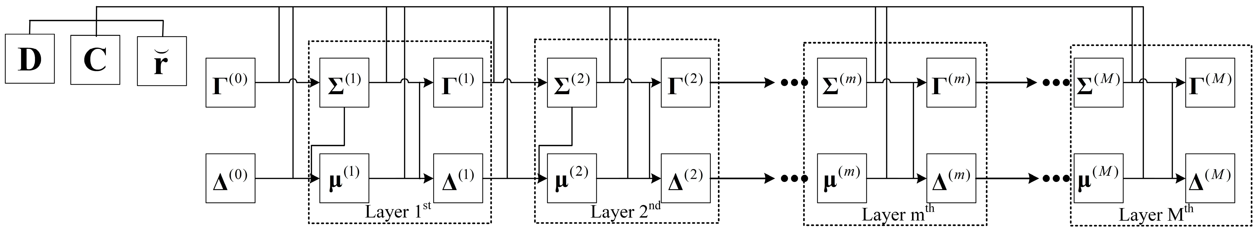
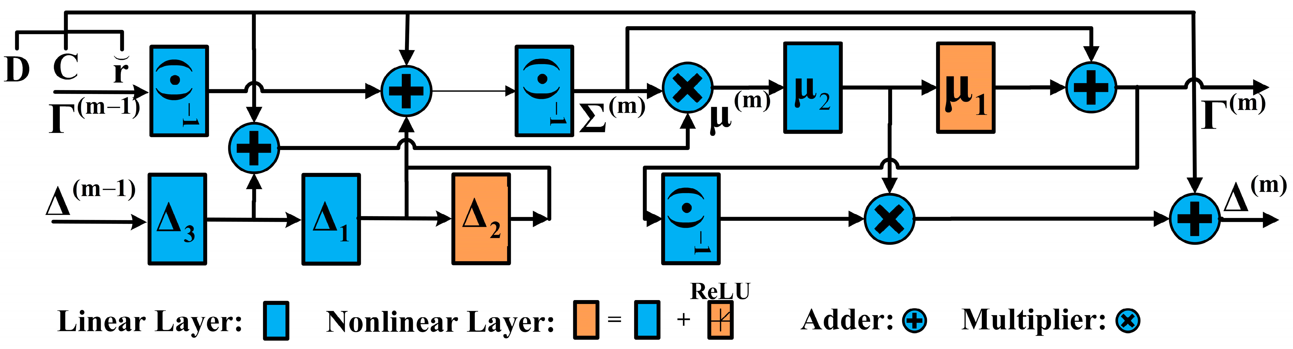
• Based on the general signal model, real-valued SBL iterative formulas are rigorously derived and adjusted, and the corresponding Bayesian deep unfolded network is constructed according to each operation in the iterative formulas rather than an entire formula;
• Off-grid errors are directly modeled and estimated by the iterative formulas, and the corresponding network architecture is considered;
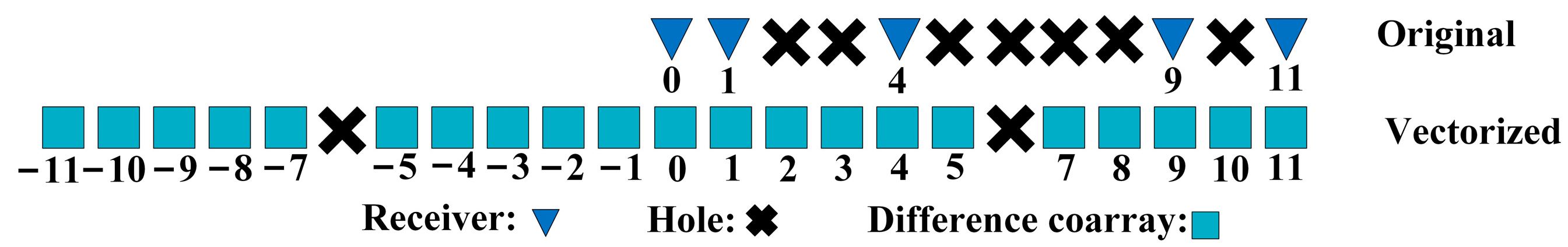
• MHA is adopted to maximize the DOF so that the estimation performance is improved.

The rest of this paper is organized as follows. In Section 2, the signal model is presented, and the DOA problem is clarified and transformed. In Section 3, SBL iterative formulas are derived, and the corresponding Bayesian deep unfolded network is constructed. Simulation results are shown in Section 4, and conclusions are drawn in Section 5.

To simplify notations, we, respectively, show functions to obtain the real/imaginary part, trace, $p$ norm, expectation, and transpose by $\Re (·)$/$\Im (·)$, $\mathrm{tr}(·)$, ${‖·‖}_p$, and $E(·)$, ${(\cdot )}^T$. We, respectively, denote real/complex number sets, conditional/marginal probability density distribution, the identity matrix, the zero vector or matrix, constant, Moore–Penrose inverse, “independent and identically distributed”, Kronecker product, and Khatri–Rao product by $ℝ$/$ℂ$, $p(a|b)$/$p(a;b)$, $I$, $0$, $const$, ${(·)}^{+}$, “i.i.d.”, $\otimes$, and $\circ$.

2. Problem Formulation

In radar detection and localization and navigation fields, the target direction is vital information in practice. Thus, how to locate signal sources well has been a research focus for more than 40 years. To be specific, array antenna receivers can receive different signals from various directions. Taking far-field radar detection as an example, adjacent antenna sensors have the same phase difference due to the plane electromagnetic wave. When the entire sensor array satisfies the configuration of MHA, a steer vector can be inferred as $a(\theta )={[\exp (-j2\pi {\xi }_1\sin (\theta )/\lambda ),\exp (-j2\pi {\xi }_2\sin (\theta )/\lambda ),\dots ,\exp (-j2\pi {\xi }_N\sin (\theta )/\lambda )]}^T\in {ℂ}^{N\times 1}$, where $\theta$ is the direction of the source signal, ${\xi }_n$ is the $n-th$ element of the MHA position set ${\mathbb{D}}_{MHA}=\left\{{\xi }_n\right|{\xi }_n={\eta }_{n}d,n=1,\dots ,N\}$, $\lambda$ is the wavelength, $d$ is the unit distance, and $N$ is the number of sensors. For all the $K$ sources from different directions $\theta =\left\{{\theta }_{k=1}^K\right\}$, the corresponding steer matrix is yielded as $A=[a({\theta }_1),\dots ,a({\theta }_K)]\in {ℂ}^{N\times K}$. $A$ is vital in DOA estimation because it implies the directions of all the sources based on the entire sensor array composed of $N$ sensors. Radio frequency signals are received by an antenna array, whose sensors transfer individually received signals to independent channels, and down conversion is conducted to produce intermediate-frequency signals, i.e., baseband signals. Later, using prior signals to execute matched filtering at time $t$, the receiver can gain the complex reflection factor of all the $K$ sources, i.e., $s(t)={[s_1(t),\dots ,s_k(t),\dots ,s_K(t)]}^T\in {ℂ}^{K\times 1}$ and $\forall k=1,\dots ,K$, where $s_k(t)$ is the product of the complex reflection coefficient and Doppler shift. Usually, the radar adopts pulse accumulation to enhance signal processing ability when the echo pulses are in the same coherent processing interval (CPI), in which little fluctuation happens between different originally received signals and processed signals. In other words, sources are motionless, and the processing signals are nearly consistent during a CPI. Overall, the entire process is briefly shown in Figure 2. The received signal at time $t$ is modeled as

$$y(t)={\displaystyle \sum _{k=1}^{K}a({\theta }_k)s_k(t)+n(t)}=A(\theta )s(t)+n(t)$$

(1)

where $y(t)\in {\mathbb{C}}^{N\times 1}$ is the received signal vector, $a({\theta }_k)={[1,\dots ,\exp (-j2\pi {\xi }_N\sin {\theta }_k/\lambda )]}^T\in {\mathbb{C}}^{N\times 1}$ is the steer vector of the $k-th$ source signal, $A(\theta )=[a({\theta }_1),\dots ,a({\theta }_K)]\in {\mathbb{C}}^{N\times K}$ is the array manifold matrix, and $n(t)\in {\mathbb{C}}^{N\times 1}$ is the vector representing the complex zero-mean Gaussian white noise with variance ${\sigma }^2$. All the complex reflection factors of source signals $s_k(t)$ are assumed to be additive complex i.i.d. Gaussian distributed with zero mean and variance ${\sigma }_k^2$, so the covariance of the received data is expressed as

$$R_y=E[y(t)y{(t)}^H]=A(\theta )R_{s}A{(\theta )}^H+{\sigma }^2{I}_N$$

(2)

where $R_s=E[s(t)s{(t)}^H]=\mathrm{diag}[{\sigma }_1^2,\dots ,{\sigma }_K^2]$. Vectorizing both sides of (2) yields

$$r=\overline{A}(\theta )\sigma +\mathrm{vec}({\sigma }^2{I}_N)$$

(3)

where $r=\mathrm{vec}(R_y)\in {\mathbb{C}}^{N^2\times 1}$, $\overline{A}(\theta )=[a{({\theta }_1)}^{\ast }\otimes a({\theta }_1),\dots ,a{({\theta }_K)}^{\ast }\otimes a({\theta }_K)]\in {\mathbb{C}}^{N^2\times K}$, and $\sigma ={[{\sigma }_1^2,\dots ,{\sigma }_K^2]}^T\in {\mathbb{R}}^{K\times 1}$. In practice, the covariance is approximated by

$${\widehat{R}}_y=\frac{1}{T}{\displaystyle \sum _{t=1}^{T}y(t)}y{(t)}^H$$

(4)

where $T$ is the number of snapshots. Compared with (3), vectorizing (4) results in an additive approximation error term $\Delta r$ [30], i.e.,

$$\widehat{r}=\overline{A}(\theta )\sigma +\mathrm{vec}({\sigma }^2{I}_N)+\Delta r$$

(5)

where $\widehat{r}=\mathrm{vec}({\widehat{R}}_y)\in {\mathbb{C}}^{N^2\times 1}$ and $\Delta r\in {\mathbb{C}}^{N^2\times 1}$ follow an asymptotic complex Gaussian distribution, i.e.,

$$p(\Delta r)=\mathcal{CN}(\Delta r|0_{N^2\times 1},R_y^H\otimes R_y/T)$$

(6)

In practice, $R_y^H\otimes R_y/T$ is replaced by $R_y^H\otimes R_y/T$ due to the unavailable $R_y$. To avoid the later influence of ${\sigma }^2$, we directly eliminate the noise term $\mathrm{vec}({\sigma }^2{I}_N)$ by a selection matrix $J\in {\mathbb{R}}^{N(N-1)\times N^2}$ [31]. Multiplying both sides of (5) yields

$$\overline{r}=\tilde{A}(\theta )x+\Delta \tilde{r}$$

(7)

where $\overline{r}=J\widehat{r}\in {\mathbb{C}}^{N(N-1)\times 1}$, $\tilde{A}(\theta )=J\overline{A}(\theta )\in {\mathbb{C}}^{N(N-1)\times K}$, $\Delta \tilde{r}=J\Delta r$$\in {\mathbb{C}}^{N(N-1)\times 1}$, and $J={[J_1^T,J_2^T,\dots ,J_i^T,\dots J_{N-1}^T]}^T$ with the $i-th$ entry $J_i$$=[0_{N\times [(i-1)N+i]},I_N,0_{N\times (N^2-iN-i)}]\in {ℝ}^{N\times N^2}$. After noise removal, $\Delta \tilde{r}$ follows $\mathcal{CN}(0_{N(N-1)\times 1},J(R_y^H\otimes R_y)J^T/T)$. Normalizing (7) so that the new approximation error follows a complex standard norm distribution and multiplying both sides of (7) by a normalization matrix $W^{-1/2}$ yields

$$\stackrel{⌢}{r}=\stackrel{⌢}{A}(\theta )\sigma +\Delta \stackrel{⌢}{r}$$

(8)

where $\stackrel{⌢}{r}=W^{-1/2}\overline{r}\in {\mathbb{C}}^{N(N-1)\times 1}$, $\stackrel{⌢}{A}(\theta )=W^{-1/2}\tilde{A}(\theta )\in {\mathbb{C}}^{N(N-1)\times K}$, $\Delta \stackrel{⌢}{r}=W^{-1/2}\Delta \tilde{r}\in {\mathbb{C}}^{N(N-1)\times 1}$, and $W=\frac{1}{T}J({\hat{R}}_y^H\otimes {\hat{R}}_y)J\in {\mathbb{C}}^{N(N-1)\times N(N-1)}$. After normalization, $\Delta \stackrel{⌢}{r}$ follows $\mathcal{CN}(0_{N(N-1)\times 1},I_{N(N-1)})$.

Let $\mathbf{\vartheta }={\mathbf{\left\{}{\vartheta }_l\mathbf{\right\}}}_{l=1}^L$ be an L-grid angular set that uniformly covers spatial range $[-\pi /2,\pi /2]$. Specially, if true sources lie on the grid, (8) can be rewritten as

$$\stackrel{⌢}{r}=\stackrel{⌣}{A}(\mathbf{\vartheta })x+\Delta \stackrel{⌢}{r}$$

(9)

where $\stackrel{⌣}{A}(\mathbf{\vartheta })=W^{-1/2}J\overline{A}(\mathbf{\vartheta }){\mathbb{C}}^{N(N-1)\times L}$ and $\overline{A}(\mathbf{\vartheta })=[a{({\vartheta }_1)}^{\ast }\otimes a({\vartheta }_1),\dots ,a{({\vartheta }_L)}^{\ast }\otimes a({\vartheta }_L)]\in {\mathbb{C}}^{N^2\times L}$. $x\in {\mathbb{R}}^{L\times 1}$ is the sparse extension of $\sigma$ with the $l-th$ element, satisfying

$$x_l=\left\{\begin{array}{c}{\sigma }_k^2, if {\vartheta }_l={\theta }_k\\ 0, elsewhere\end{array}\right.$$

(10)

Obviously, $x$ is sparse with many zero elements since $L$ is usually large enough for high estimation accuracy. Despite large $L$ being adopted, there still exists errors if true sources are off-grid, i.e., ${\vartheta }_l\ne {\theta }_k$ and $\forall l=1,\dots ,L$. Considering that, we approximate the $k-th$ true source DOA ${\theta }_k$ by the Taylor expansion at the corresponding nearest gird ${\vartheta }_{l_k}$, i.e.,

$$a({\theta }_k)\approx a({\vartheta }_{l_k})+b({\vartheta }_{l_k})({\theta }_k-{\vartheta }_{l_k})$$

(11)

where $b({\vartheta }_{l_k})=[a({\vartheta }_{l_k}){]}^{\prime }$ is the derivative of $a({\vartheta }_{l_k})$ with respect to ${\vartheta }_{l_k}$. For simplicity, the $i-th$ element of $\delta ={[{\delta }_1,\dots ,{\delta }_L]}^T$ is introduced as

$${\delta }_l=\left\{\begin{array}{c}{\theta }_k-{\vartheta }_{l_k}, if l=l_k\\ 0, elsewhere\end{array}\right.$$

(12)

where ${\delta }_l$ is limited in $[-r/2,r/2]$ and $r$ is the gird interval. If ${\delta }_l$ exceeds the range, $\pm r/2$ is assigned to ${\delta }_l$. Using (11) and (12) and ignoring the quadratic term with respect to ${\delta }_l$, the following equation approximately holds:

$$\begin{array}{l}a{({\theta }_k)}^{\ast }\otimes a({\theta }_k)={[a({\vartheta }_{l_k})+b({\vartheta }_{l_k}){\delta }_l]}^{\ast }[a({\vartheta }_{l_k})+b({\vartheta }_{l_k}){\delta }_l]\\ \approx a{({\vartheta }_{l_k})}^{\ast }\otimes a({\vartheta }_{l_k})+[b{({\vartheta }_{l_k})}^{\ast }\otimes a({\vartheta }_{l_k})+a{({\vartheta }_{l_k})}^{\ast }\otimes b({\vartheta }_{l_k})]{\delta }_l\end{array}$$

(13)

Let $\delta ={[{\delta }_1,\dots ,{\delta }_L]}^T\in {\mathbb{R}}^{L\times 1}$ and $\Delta =\mathrm{diag}(\delta )\in {\mathbb{R}}^{L\times L}$. For all the $K$ sources, (13) is extended to

$$\overline{A}(\theta )\approx \Phi (\mathbf{\vartheta })=\overline{A}(\mathbf{\vartheta })+[A{(\mathbf{\vartheta })}^{\ast }\circ B(\mathbf{\vartheta })+B{(\mathbf{\vartheta })}^{\ast }\circ A(\mathbf{\vartheta })]\Delta$$

(14)

where $\Phi (\mathbf{\vartheta })\in {\mathbb{C}}^{N^2\times L}$, $A(\mathbf{\vartheta })=[a({\vartheta }_1),\dots ,a({\vartheta }_L)]\in {\mathbb{C}}^{N\times L}$, $B(\mathbf{\vartheta })=[b({\vartheta }_1),\dots ,b({\vartheta }_L)]\in {\mathbb{C}}^{N\times L}$. Therefore, (9) is rewritten as

$$\stackrel{⌢}{r}=\psi (\mathbf{\vartheta })x+\Delta \stackrel{⌢}{r}$$

(15)

where $\psi (\mathbf{\vartheta })=W^{-1/2}J\Phi (\mathbf{\vartheta })\in {\mathbb{C}}^{N(N-1)\times L}$. As neural networks of deep unfolding are originally designed for real-valued data, we transform (15) into a real-valued equation as

$$\stackrel{⌣}{r}=\stackrel{⌣}{\psi }(\mathbf{\vartheta })x+\Delta \stackrel{⌣}{r}$$

(16)

where $\stackrel{⌣}{r}=\left[\begin{array}{c}\Re (\stackrel{⌢}{r})\\ \Im (\stackrel{⌢}{r})\end{array}\right]\in {\mathbb{R}}^{2N(N-1)\times 1}$, $D=\left[\begin{array}{c}\Re (W^{-1/2}J[A{(\mathbf{\vartheta })}^{\ast }\circ B(\mathbf{\vartheta })+B{(\mathbf{\vartheta })}^{\ast }\circ A(\mathbf{\vartheta })])\\ \Im (W^{-1/2}J[A{(\mathbf{\vartheta })}^{\ast }\circ B(\mathbf{\vartheta })+B{(\mathbf{\vartheta })}^{\ast }\circ A(\mathbf{\vartheta })])\end{array}\right]\in {\mathbb{R}}^{2N(N-1)\times L}$, $C=\left[\begin{array}{c}\Re (W^{-1/2}J\overline{A}(\mathbf{\vartheta }))\\ \Im (W^{-1/2}J\overline{A}(\mathbf{\vartheta }))\end{array}\right]\in {\mathbb{R}}^{2N(N-1)\times L}$, $\stackrel{⌣}{\psi }(\mathbf{\vartheta })=C+D\Delta$, and $\Delta \stackrel{⌣}{r}=\left[\begin{array}{c}\Re (\Delta \stackrel{⌢}{r})\\ \Im (\Delta \stackrel{⌢}{r})\end{array}\right]\in {\mathbb{R}}^{2N(N-1)\times 1}$.

Overall, the DOA estimation problem is equivalently cast as a sparse recovery problem for solving real-valued $x$ and $\delta$ with real and imaginary parts of known complex quantities $\stackrel{⌢}{r}$, $A(\mathbf{\vartheta })$, $B(\mathbf{\vartheta })$, and $\overline{A}(\mathbf{\vartheta })$.

3. Proposed Method

In this section, the DOA estimation is realized in accordance with the real-valued framework in (16) by Bayesian inference based on the posterior. The proposed method is developed via an iterative procedure to jointly recover the sparse support $x$ and the grid mismatch error $\delta$.

3.1. Bayesian Inference

As widely known, Bayesian inference is based on the posterior decided by likelihood and priors. According to (16), the likelihood is

$$p(\stackrel{⌣}{r}|x;\Delta )=\mathcal{N}(\stackrel{⌣}{r}|\stackrel{⌣}{\psi }(\mathbf{\vartheta })x,I_{2N(N-1)})$$

(17)

Then, i.i.d. Gaussian priors are assigned to all the elements of $x$ as follows:

$$p(x;\Gamma )=\mathcal{N}(x|0_L,\Gamma )$$

(18)

where $\Gamma \in {\mathbb{R}}^{L\times L}$ is a diagonal matrix, i.e., $\Gamma =\mathrm{diag}(\gamma )$ and $\gamma ={[{\gamma }_1,\dots ,{\gamma }_L]}^T\in {\mathbb{R}}^{L\times 1}$. Remark: $\gamma$ is finally regarded as the solved $x$ since $\gamma$ represents the potential source power so as to reflect the potential source location.

According to the Bayesian formula, the posterior is

$$p(x|\stackrel{⌣}{r};\Delta ,\Gamma )=\frac{p(\stackrel{⌣}{r}|x;\Delta )p(x;\Gamma )}{{\displaystyle \int p(\stackrel{⌣}{r}|x;\Delta )p(x;\Gamma )dx}}$$

(19)

(19) is analytically solved to be a Gaussian distribution with mean and variance as follows:

$$\begin{array}{l}\mu =\Sigma \stackrel{⌣}{\psi }{(\mathbf{\vartheta })}^T\stackrel{⌣}{r}\\ \Sigma ={({\Gamma }^{-1}+\stackrel{⌣}{\psi }{(\mathbf{\vartheta })}^T\stackrel{⌣}{\psi }(\mathbf{\vartheta }))}^{-1}\end{array}$$

(20)

where $\mu \in {\mathbb{R}}^{L\times 1}$ and $\Sigma \in {\mathbb{R}}^{L\times L}$. Please refer to Appendix A for the derivation. Finally, Bayesian inference is realized based on the maximum a posteriori (MAP) criterion. Specifically, we update hyperparameters $\Gamma$ and $\Delta$ to maximize the logarithmic expectation of (19), i.e.,

$$\begin{array}{l}\Gamma =\mathrm{diag}(\gamma )=\underset{\Gamma }{\arg \max }\{\mathrm{E}[\ln p(x|\stackrel{⌣}{r};\Delta ,\Gamma )]\}\\ \Delta =\mathrm{diag}(\delta )=\underset{\Delta }{\arg \max }\{\mathrm{E}[\ln p(x|\stackrel{⌣}{r};\Delta ,\Gamma )]\}\end{array}$$

(21)

Using (21), $\gamma$ and $\delta$ are analytically solved as follows:

$$\begin{array}{l}\gamma =\mathrm{diag}(\mu {\mu }^T+\Sigma )\\ \delta =\mathrm{diag}(D^{+}\stackrel{⌣}{r}{\mu }^T{(\mu {\mu }^T+\Sigma )}^{-1}-D^{+}\mathbf{C})\end{array}$$

(22)

Please refer to Appendix B for the derivation.

Overall, the SBL algorithm is summarized in

Table 1. The proposed method is named Algorithm 1.

Initialize $\delta$, $\gamma$, ${\epsilon }^{(0)}$, error tolerance $\epsilon$, set elements in $\delta$ or $\gamma$ as small and the same values. While ${\epsilon }^{(k)}>\epsilon$ do: compute $\mu$ and $\Sigma$ according to (20). compute $\gamma$ and $\delta$ according to (22). ${\epsilon }^{(k)}=‖{\gamma }^{(k+1)}-{\gamma }^{(k)}‖/‖{\gamma }^{(k)}‖$. $k=k+1$. End While Return $\gamma$ and $\delta$. Output refined DOAs.

.

The proposed method has guaranteed convergence since the posterior is bound to increase at each iteration. However, the SBL converges quite slowly, so we construct the corresponding deep unfolded network based on Algorithm 1 to accelerate the convergence rate.

3.2. Deep Unfolding

In order to unfold Algorithm 1 into deep neural network architecture, iterative equations (20) and (22) are rewritten as

$$\begin{array}{l}{\Sigma }^{(m)}={\{{\mathbf{C}}^T\mathbf{C}+{({\Gamma }^{(m-1)})}^{-1}+\underset{{\Delta }_1}{\underbrace{{\mathbf{C}}^{T}D{\Delta }^{(m-1)}+{({\Delta }^{(m-1)})}^T{D}^T\mathbf{C}}}+\underset{{\Delta }_2}{\underbrace{{({\Delta }^{(m-1)})}^T{D}^{T}D{\Delta }^{(m-1)}}}\}}^{-1}\\ {\mu }^{(m)}={\Sigma }^{(m)}(\mathbf{C}\stackrel{⌣}{\mathrm{r}}+\underset{{\Delta }_3}{\underbrace{D{\Delta }^{(m-1)}\stackrel{⌣}{r}}})\\ {\Gamma }^{(m)}=\underset{{\mu }_1}{\underbrace{{\mu }^{(m)}{({\mu }^{(m)})}^T}}+{\Sigma }^{(m)}\\ {\Delta }^{(m)}=\underset{{\mu }_2}{\underbrace{2D^{+}\stackrel{⌣}{r}{({\mu }^{(m)})}^T}}{({\Gamma }^{(m)})}^{-1}-D^{+}\mathbf{C}\end{array}$$

(23)

via linear transformation, where $m=1,\dots ,M$ denotes the $m-th$ iteration. Remark: In our deep unfolded neural networks, ${\Delta }_1$, ${\Delta }_3$, ${\mu }_2$, matrix inversion, and matrix transposition with respect to iterative hyperparameters are fitted by linear layers since they are linear transformations, while the nonlinear quadratic terms ${\Delta }_2$ and ${\mu }_1$ are fitted by nonlinear layers. Constant terms are input, and the rest in (23) are realized by adders and multipliers. Specifically, the constructed network architecture is shown in Figure 3 and Figure 4.

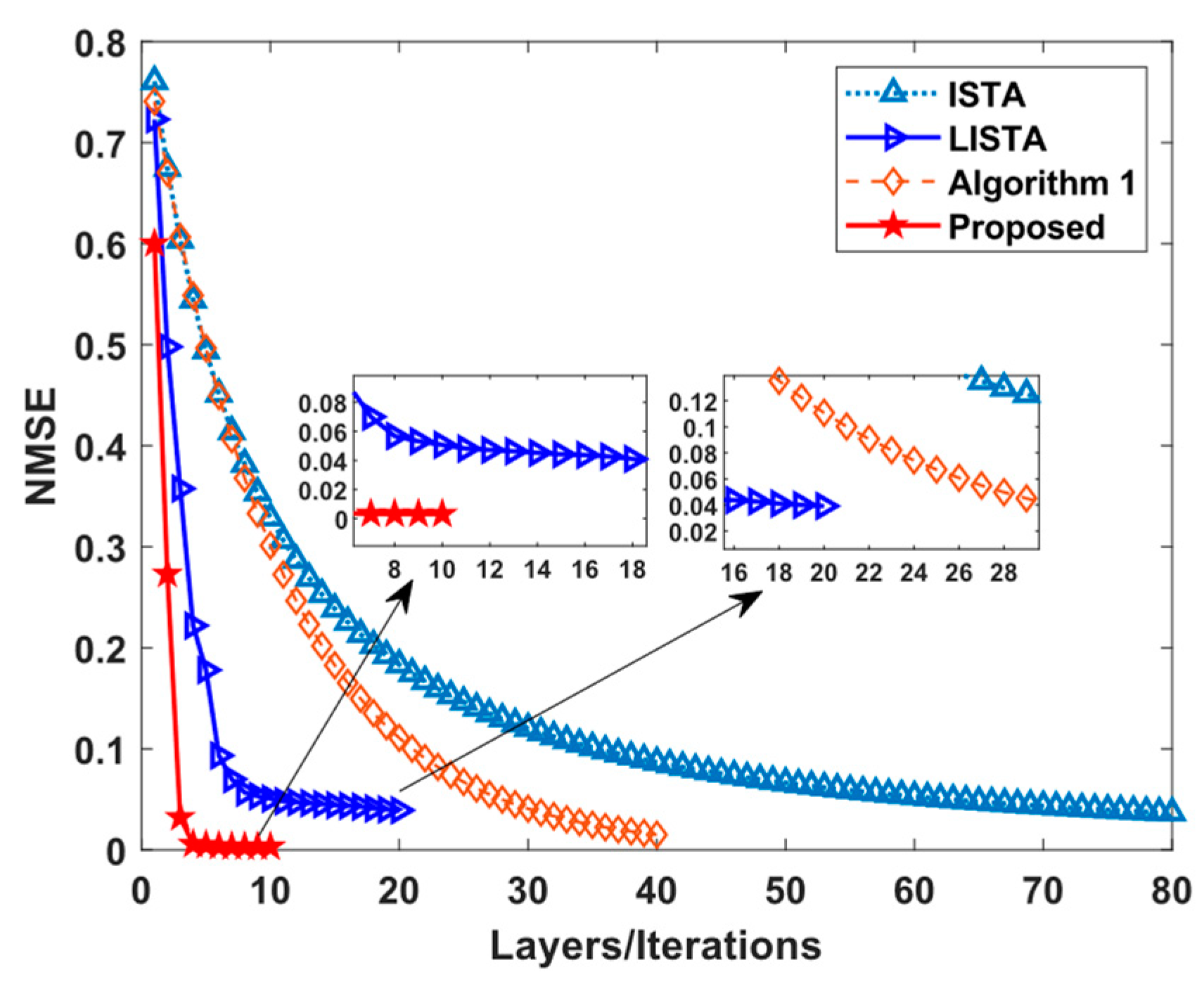
4. Numerical Simulation

In this section, the superiority of the proposed method is fully evaluated by three simulations.

Simulation 1 tests the convergence rates of the 10-layer proposed method and Algorithm 1, ISTA [32], and 20-layer LISTA [9]. Simulation conditions are as follows. (ⅰ) Baseline conditions: Inter(R) Xeon(R) Platinum 8270 CPU @ 2.70 GHz, three uncorrelated source signals from random on-grid angles $\{-{20}^{\circ },5^{\circ },{30}^{\circ }\}$ with random off-grid gaps $\{{0.13}^{\circ },{0.45}^{\circ },{0.32}^{\circ }\}$, grid interval $1^{\circ }$, $SNR=20\mathrm{dB}$, $T=60$ snapshots, $N=6$ sensors with position set ${\mathbb{D}}_{MHA}=\{0,1,8,11,13,17\}$, and grid range $[-{90}^{\circ },{90}^{\circ }]$. (ⅱ) Neural network training conditions: NVIDIA Quadro RTX 8000 GPU, on-gird space $[-{90}^{\circ },{90}^{\circ }]$ with $1^{\circ }$ interval, and off-grid space $[-{0.5}^{\circ },{0.5}^{\circ })$ with ${0.01}^{\circ }$ interval; thus, the total is 18,100 labels, and each label corresponds to 10 samples so as to yield 181,000 samples $\stackrel{⌣}{r}$, epoch 500, batch size 32, a training–validating ratio of 8:2, an Adam optimizer with a learning rate of 0.001, and a designed normalized mean square error (NMSE) function as a loss function. The NMSE is defined as

$$NMSE=\frac{1}{2P}{\displaystyle \sum _{p=1}^P({‖\widehat{x}-x‖}_2^2/{‖x‖}_2^2+{‖\widehat{\delta }-\delta ‖}_2^2/{‖\delta ‖}_2^2)}$$

(24)

where $P$ is the batch size of the validation set. $\widehat{x}$ and $\widehat{\delta }$ are the estimated values of the validated labels $x$ and $\delta$ yielded by (ⅰ) baseline conditions.

The simulation results are depicted in Figure 5. Intuitively, the algorithms based on deep unfolding, i.e., LISTA and the proposed method, converge faster than their original algorithms, i.e., ISTA and Algorithm 1. The proposed method requires fewer layers and achieves a lower bound than LISTA at convergence, which implies the proposed method has a faster convergence rate and better sparse recovery ability. The simulation results can be explained by the fact that the deep unfolded techniques indeed enable accelerating convergence, and SBL converges faster than ISTA originally. Owing to the reasonable and effective network architecture, the proposed method achieves remarkable convergence performance.

The following simulations focus on the root-mean-square error (RMSE) performance comparison of LISTA, FAAN-MUSIC [33], RVSBL [34], StructCovMLE [35], CRLB [36], and the proposed method. The RMSE is defined as

$$RMSE=\sqrt{\frac{1}{M_{c}K}{\displaystyle \sum _{m_c=1}^{M_c}{\displaystyle \sum _{k=1}^K{({\widehat{\theta }}_{m_c,k}-{\theta }_k)}^2}}}$$

(25)

where $M_c=200$ is the Monte Carlo number, ${\widehat{\theta }}_{m_c,k}$ is the estimated angle for the $k-th$ source in the $m_c-th$ trial, and ${\theta }_k$ is the true angle for the $k-th$ source.

Simulation 2 investigates the RMSE performance with respect to SNRs. As shown in Figure 6, the proposed method realizes a lower RMSE than others and approaches the CRLB. In particular, the proposed method outperforms RVSBL, which indicates that the used MHA indeed improves DOA estimation accuracy. On the one hand, the proposed method inherits the advantage of SBL, i.e., excellent sparsity recovery ability. On the other hand, the real-valued transformation further enhances its ability.

Simulation 3 tests the RMSE performance with respect to the number of snapshots. The simulation results in Figure 7 show that the proposed method is robust to snapshot varying, i.e., it requires slight sampling data but achieves high estimation accuracy, which can be explained by the fact that data-driven methods have powerful mapping and fitting abilities. Undoubtedly, the constructed deep unfolded network realizes excellent mapping effects, and, simultaneously, prominent generalization capability.

Simulation 4 examines the RMSE performance with respect to the number of sources. Here, all the source angles are uniformly selected from the interval of $[-{90}^{\circ },{90}^{\circ }]$. Intuitively, in Figure 8, all the algorithms inevitably suffer performance reduction, but the proposed method still outperforms others over the whole range of various numbers of sources. The results indicate that the proposed method has the potential to locate more sources when the angle accuracy is not strictly constrained.

Simulation 5 focuses on the RMSE performance with respect to the number of sensors. Notice that the number of sensors ranges from 4 to 8. The reason for this is that the MUSCI-based method, i.e., FAAN–MUSIC, can only locate maximal $N-1$ sources with $N$ sensors. Thus, $N-1\ge 3$ must be satisfied so that FAAN–MUSIC works normally. In the proposed method, the adopted MHA position set is ${\mathbb{D}}_{MHA}=\{0,1,4,9,15,22,32,34\}$ and contains the maximized eight sensors. In Figure 9, the proposed method achieves the fewest RMSEs. This result can be explained by the fact that the proposed method can inherit the ability of SBL to handle highly underdetermined problems, and the adopted MHA indeed plays an important role in improving estimation accuracy.

Based on Simulation 2, Simulation 6 examines the average computational time for each Monte Carlo trial. As shown in

Table 2. Computational time of the algorithms.

Algorithms	Computational Time
FAAN-MUSIC	1.223 s
RVSBL	0.294 s
StructCovMLE	0.537 s
LISTA	0.00137 s
Proposed	0.00472 s

, the proposed method runs faster than others, except for LISTA, which proves that the used deep unfolded network indeed improves SBL efficiency significantly. Remark: The result, i.e., the proposed method, is slower than LISTA and has no conflict against the conclusions in Simulation 1 because the computational complexity of each layer of the proposed method is larger than that in LISTA.

5. Conclusions

In this paper, a Bayesian deep unfolded network is constructed according to our derived SBL iterative formulas and is based on the adopted minimum hole array for a high estimation accuracy. Simulation results sufficiently illustrate the superiority of the proposed method, such as its high convergence rate and excellent estimation performance. On the one hand, the proposed method inherits the advantages of SBL, e.g., robustness to various snapshots, excellent sparsity performance, and the ability to handle underdetermined cases. On the other hand, the proposed method reserves and extends the superiority of deep learning, such as steady estimation ability owing to real-valued data and fast convergence ability. More importantly, this paper empirically proves the advantages of deep unfolding again, though rigorously theoretical identification is not provided.

References

1. Krim, H.; Viberg, M. Two decades of array signal processing research: The parametric approach. IEEE Signal Proc. Mag. 1996, 13, 67–94. [Google Scholar] [CrossRef]
2. Pesavento, M.; Trinh-Hoang, M.; Viberg, M. Three More Decades in Array Signal Processing Research: An optimization and structure exploitation perspective. IEEE Signal Proc. Mag. 2023, 40, 92–106. [Google Scholar] [CrossRef]
3. Liu, W.; Haardt, M.; Greco, M.S.; Mecklenbräuker, C.F.; Willett, P. Twenty-Five Years of Sensor Array and Multichannel Signal Processing: A review of progress to date and potential research directions. IEEE Signal Proc. Mag. 2023, 40, 80–91. [Google Scholar] [CrossRef]
4. Purwins, H.; Li, B.; Virtanen, T.; Schlüter, J.; Chang, S.Y.; Sainath, T. Deep learning for audio signal processing. IEEE J. Sel. Top. Signal Process. 2019, 13, 206–219. [Google Scholar] [CrossRef]
5. Krizhevsky, A.; Sutskever, I.; Hinton, G.E. Imagenet classification with deep convolutional neural networks. Adv. Neural Inf. Process. Syst. 2012, 25, 84–90. [Google Scholar] [CrossRef]
6. LeCun, Y.; Bengio, Y.; Hinton, G. Deep learning. Nature 2015, 521, 436–444. [Google Scholar] [CrossRef] [PubMed]
7. Nielsen, I.E.; Dera, D.; Rasool, G.; Ramachandran, R.P.; Bouaynaya, N.C. Robust explainability: A tutorial on gradient-based attribution methods for deep neural networks. IEEE Signal Proc. Mag. 2022, 39, 73–84. [Google Scholar] [CrossRef]
8. Monga, V.; Li, Y.; Eldar, Y.C. Algorithm unrolling: Interpretable, efficient deep learning for signal and image processing. IEEE Signal Proc. Mag. 2021, 38, 18–44. [Google Scholar] [CrossRef]
9. Gregor, K.; LeCun, Y. Learning fast approximations of sparse coding. In Proceedings of the 27th International Conference on International Conference on Machine Learning, Haifa, Israel, 21–24 June 2010; pp. 399–406. [Google Scholar]
10. Hershey, J.R.; Roux, J.L.; Weninger, F. Deep unfolding: Model-based inspiration of novel deep architectures. arXiv 2014, arXiv:1409.2574. [Google Scholar]
11. Liu, J.; Chen, X. ALISTA: Analytic weights are as good as learned weights in LISTA. In Proceedings of the International Conference on Learning Representations, New Orleans, LA, USA, 6–9 May 2019. [Google Scholar]
12. Chen, X.; Liu, J.; Wang, Z.; Yin, W. Theoretical linear convergence of unfolded ISTA and its practical weights and thresholds. Adv. Neural Inf. Process. Syst. 2018, 31. [Google Scholar]
13. Zhang, J.; Ghanem, B. ISTA-Net: Interpretable optimization-inspired deep network for image compressive sensing. In Proceedings of the IEEE Conference on Computer Vision and Pattern Recognition, Salt Lake City, UT, USA, 18–22 June 2018; pp. 1828–1837. [Google Scholar]
14. Sun, J.; Li, H.; Xu, Z. Deep ADMM-Net for compressive sensing MRI. Adv. Neural Inf. Process. Syst. 2016, 29, 10–18. [Google Scholar]
15. Su, X.; Liu, Z.; Shi, J.; Hu, P.; Liu, T.; Li, X. Real-valued deep unfolded networks for off-grid DOA estimation via nested array. IEEE Trans. Aerosp. Electron. Syst. 2023, 59, 4049–4062. [Google Scholar] [CrossRef]
16. Su, X.; Hu, P.; Liu, Z.; Shi, J.; Li, X. Deep alternating projection networks for gridless DOA estimation with nested array. IEEE Signal Proc. Let. 2022, 29, 1589–1593. [Google Scholar] [CrossRef]
17. Wu, L.; Liu, Z.M.; Liao, J. DOA estimation using an unfolded deep network in the presence of array imperfections. In Proceedings of the 2022 7th International Conference on Signal and Image Processing (ICSIP), Suzhou, China, 20–22 July 2022; pp. 182–187. [Google Scholar]
18. Tang, H.; Zhang, Y.; Luo, J.; Zhang, Y.; Huang, Y.; Yang, J. Sparse DOA Estimation Based on a Deep Unfolded Network for MIMO Radar. In Proceedings of the IGARSS 2023—2023 IEEE International Geoscience and Remote Sensing Symposium, Pasadena, CA, USA, 16–21 July 2023; pp. 5547–5550. [Google Scholar]
19. Li, Y.; Wang, X.; Olesen, R.L. Unfolded deep neural network (UDNN) for high mobility channel estimation. In Proceedings of the 2021 IEEE Wireless Communications and Networking Conference (WCNC), Nanjing, China, 29 March–1 April 2021; pp. 1–6. [Google Scholar]
20. Johnston, J.; Wang, X. Model-based deep learning for joint activity detection and channel estimation in massive and sporadic connectivity. IEEE Trans. Wirel. Commun. 2022, 21, 9806–9817. [Google Scholar] [CrossRef]
21. Kang, K.; Hu, Q.; Cai, Y.; Yu, G.; Hoydis, J.; Eldar, Y.C. Mixed-timescale deep-unfolding for joint channel estimation and hybrid beamforming. IEEE J. Sel. Areas Commun. 2022, 40, 2510–2528. [Google Scholar] [CrossRef]
22. Tipping, M.E. Sparse Bayesian learning and the relevance vector machine. J. Mach. Learn. Res. 2001, 1, 211–244. [Google Scholar]
23. Li, N.; Zhang, X.K.; Zong, B.; Lv, F.; Xu, J.; Wang, Z. An off-grid direction-of-arrival estimator based on sparse Bayesian learning with three-stage hierarchical Laplace priors. Signal Process. 2024, 218, 109371. [Google Scholar] [CrossRef]
24. Gong, Z.; Su, X.; Hu, P.; Liu, S.; Liu, Z. Deep Unfolding Sparse Bayesian Learning Network for Off-Grid DOA Estimation with Nested Array. Remote Sens. 2023, 15, 5320. [Google Scholar] [CrossRef]
25. Wan, Q.; Fang, J.; Huang, Y.; Duan, H.; Li, H. A variational Bayesian inference-inspired unrolled deep network for MIMO detection. IEEE Trans. Signal Process. 2022, 70, 423–437. [Google Scholar] [CrossRef]
26. Hu, Q.; Shi, S.; Cai, Y.; Yu, G. DDPG-driven deep-unfolding with adaptive depth for channel estimation with sparse Bayesian learning. IEEE Trans. Signal Process. 2022, 70, 4665–4680. [Google Scholar] [CrossRef]
27. Gao, J.; Cheng, X.; Li, G.Y. Deep Unfolding-Based Channel Estimation for Wideband TeraHertz Near-Field Massive MIMO Systems. arXiv 2023, arXiv:2308.13381. [Google Scholar]
28. Linebarger, D.A.; Sudborough, I.H.; Tollis, I.G. Difference bases and sparse sensor arrays. IEEE Trans. Inf. Theory 1993, 39, 716–721. [Google Scholar] [CrossRef]
29. Pal, P.; Vaidyanathan, P.P. Nested arrays: A novel approach to array processing with enhanced degrees of freedom. IEEE Trans. Signal Process. 2010, 58, 4167–4181. [Google Scholar] [CrossRef]
30. Ottersten, B.; Stoica, P.; Roy, R. Covariance matching estimation techniques for array signal processing applications. Digit. Signal Process. 1998, 8, 185–210. [Google Scholar] [CrossRef]
31. Yang, J.; Liao, G.; Li, J. An efficient off-grid DOA estimation approach for nested array signal processing by using sparse Bayesian learning strategies. Signal Process. 2016, 128, 110–122. [Google Scholar] [CrossRef]
32. Beck, A.; Teboulle, M. A fast iterative shrinkage-thresholding algorithm for linear inverse problems. SIAM J. Imaging Sci. 2009, 2, 183–202. [Google Scholar] [CrossRef]
33. Stoica, P.; Babu, P. Low-rank covariance matrix estimation for factor analysis in anisotropic noise: Application to array processing and portfolio selection. IEEE Trans. Signal Process. 2023, 71, 1699–1713. [Google Scholar] [CrossRef]
34. Das, A. Real-valued sparse Bayesian learning for off-grid direction-of-arrival (DOA) estimation in ocean acoustics. IEEE J. Ocean. Eng. 2020, 46, 172–182. [Google Scholar] [CrossRef]
35. Pote, R.R.; Rao, B.D. Maximum likelihood-based gridless doa estimation using structured covariance matrix recovery and sbl with grid refinement. IEEE Trans. Signal Process. 2023, 71, 802–813. [Google Scholar] [CrossRef]
36. Stoica, P.; Larsson, E.G.; Gershman, A.B. The stochastic CRB for array processing: A textbook derivation. IEEE Signal Process. Lett. 2001, 8, 1448–1501. [Google Scholar] [CrossRef]
Figure 1. Minimum hole array of five sensor receivers.
Electronics 13 02139 g001
Figure 2. Flowchart of radar signal processing for DOA estimation.
Electronics 13 02139 g002
Figure 3. Scheme of the proposed Bayesian deep unfolded network.
Electronics 13 02139 g003
Figure 4. Scheme of the m-th layer of the Bayesian deep unfolded network.
Electronics 13 02139 g004
Figure 5. NMSE versus layers/iterations.
Electronics 13 02139 g005
Figure 6. RMSE versus SNR.
Electronics 13 02139 g006
Figure 7. RMSE versus the number of snapshots.
Electronics 13 02139 g007
Figure 8. RMSE versus the number of sources.
Electronics 13 02139 g008
Figure 9. RMSE versus the number of sensors.
Electronics 13 02139 g009