Automatic Modulation Recognition Method Based on Phase Transformation and Deep Residual Shrinkage Network

Abstract

Automatic Modulation Recognition (AMR) is currently a research hotspot, and research under low Signal-to-Noise Ratio (SNR) conditions still poses certain challenges. This paper proposes an AMR method based on phase transformation and deep residual shrinkage network to improve recognition accuracy. Firstly, the raw I/Q data from the benchmark dataset RML2016.10a are used as the input. Then, an end-to-end modulation recognition is performed using the model. Phase transformation is used to correct the raw I/Q data and reduce the interference of phase shift on modulation recognition. Convolutional neural network (CNN) and Gate Recurrent Unit (GRU) extract the spatial and temporal features of the modulation signal, respectively. The improved deep residual shrinkage network is added after CNN to eliminate unimportant features through soft thresholding. Finally, the proposed model is trained and tested. The experimental results show that the proposed model notably reduces the number of parameters compared to other models, effectively improving the recognition accuracy under low SNR conditions. The average recognition accuracy reaches 62.46%, and the highest recognition accuracy reaches 92.41%.

1. Introduction

AMR can be used to identify the modulation style of intercepted signals, providing a prerequisite for information acquisition. As a key method in signal detection and demodulation, AMR has played a good role in multiple fields [1], such as spectrum detection, spectrum sensing, cognitive radio, etc. [2], and has become a research hotspot in recent years. As communication technology advances by leaps and bounds, the signal transmission environment has become increasingly complex, and the transmission process is susceptible to adverse factors such as noise, multipath fading, frequency offset, etc. In order to meet different communication needs, more and more communication signal modulation styles are being studied and applied. These have brought huge challenges to AMR technology. Therefore, designing modulation recognition models with good performance in poor wireless environments has become particularly urgent and important.

Traditional AMR method consists of two components: likelihood-theory-based AMR (LB-AMR) [3,4,5] and feature-based AMR (FB-AMR) [6]. The LB-AMR method is optimal under the Bayesian assumption, but its computational complexity is high and requires known channel parameter scenarios. FB-AMR methods first learn representative features, and then use features to distinguish modulation styles. The features used include envelope characteristics [7], wavelet transform features [8], and high-order cumulants [9]. Algorithms include artificial neural networks [10], support vector machines [11], and decision trees [12]. Although FB-AMR methods have lower computational complexity, their feature design requires strong professional knowledge and features are not universally representative, making them susceptible to factors such as noise. Compared to LB-AMR methods and FB-AMR methods, deep learning (DL)-based AMR methods have more advantages in terms of recognition accuracy and implementation complexity.

A convolutional radio modulation recognition network was first proposed in [13], which performs better than classifiers based on expert features. Drawing inspiration from residual networks (Resnet) and Densely Connected Networks (Densenet) in the field of image processing, the corresponding modulation recognition models were established in [14]. Using skip connections to enhance feature propagation between different layers, a Convolutional Long Short-term Deep Neural Network (CLDNN) model was also introduced. The inputs of the above network model are all raw I/Q data, which makes it difficult to effectively utilize relevant expert features, such as high-order cumulants, spectrograms, constellation maps, etc. In response to this issue, Zeng et al. [15] conducted research on time–frequency analysis methods and used short-time discrete Fourier transform to obtain the frequency spectrum of the signal. Peng et al. [16] converted radio signals into constellation maps and utilized the color image processing capabilities of AlexNet and GoogLeNet for feature extractions and style classifications. He et al. [17] first used continuous wavelet transform to process the received signal, and then used a model to process the obtained image, which performed well under low SNR. Although the recognition accuracy of the above models has been improved to a certain extent, in practical applications, obtaining multiple forms of signals is a complex task, and different types of inputs can lead to more complex network structures, larger model sizes, and longer computation times, which thus affect the algorithm performance.

Due to the small memory capacity and limited computing resources of edge devices [18], such as IoT devices and drones [19], it is not possible to deploy larger network models. However, in practical applications, there is a strong demand for the processing power and reaction time of the models. Hermawan et al. [20] improved the network structure by combining convolutional layers, pooling layers, and Gaussian noise layers, and added Dropout algorithm for regularization to prevent overfitting during network training. It used fewer convolutional kernels in each layer of the network to reduce the network processing time. Drawing inspiration from the effectiveness of Long Short-Term Memory (LSTM) networks in processing time series correlations, Rajendran et al. [21] first preprocessed the original I/Q data to obtain amplitude and phase information, and then used double-layer LSTM to extract features. The average recognition accuracy was high in the range of 0–20 dB SNR, and the model was well simplified. Njoku et al. [22] proposed an efficient hybrid deep learning model, consisting of CNN and GRU, using Gaussian dropout layers and small convolutional kernel sizes to accelerate the feature extraction process and prevent gradient vanishing problems. Xu et al. [23] designed a complex valued neural network for modulation recognition. The above network models ignore an issue: CNN only performs data fitting and does not have noise reduction strategies in the sense of signal processing. As a result, the features generated by noise will also have a certain mapping relationship in the model. Therefore, the above network models are affected by noise factors, and the average recognition accuracy on the benchmark dataset is not high. The recognition accuracy needs further research under low SNR. Zhao et al. [24] developed a new deep learning idea, namely deep residual shrinkage network. By incorporating the soft threshold module as a nonlinear transformation layer into the network model for training, it effectively eliminates noise-related features and enhances the model’s feature extraction ability when processing high noise vibration signals. Based on this idea, this paper improves the deep residual shrinkage network by introducing a scaling factor, multiplying it with the soft threshold in the model, and thus places the improved deep residual shrinkage network behind the CNN to preserve or eliminate the feature values obtained from the convolutional process, thereby enhancing the signal denoising effect. On this basis, we design an efficient model based on phase transformation and deep residual shrinkage network, using raw I/Q data for end-to-end modulation recognition. The model has fewer parameters, shorter training time, and to some extent improves recognition accuracy.

The main contributions of this paper are as follows:

(1)

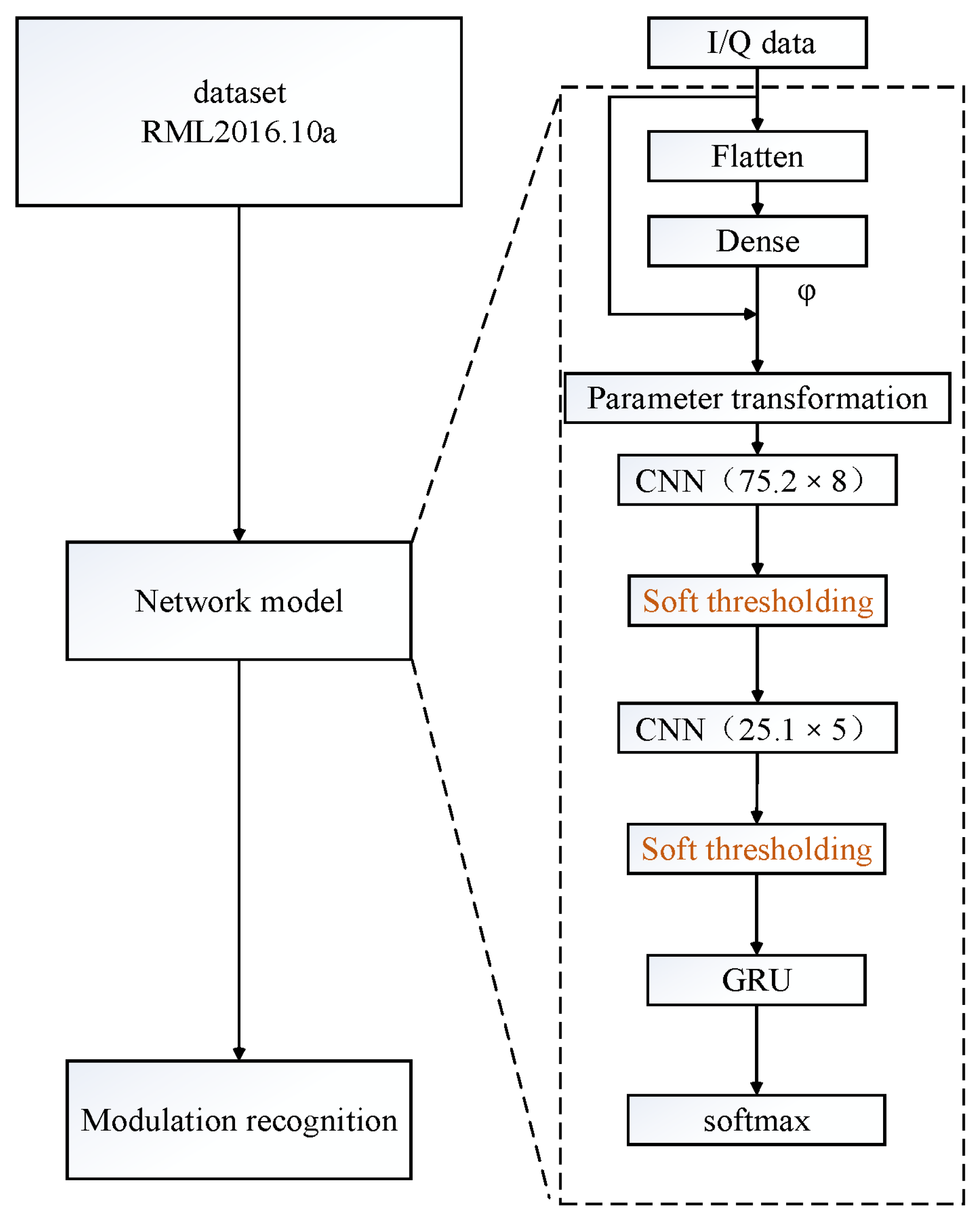
This paper proposes an AMR model based on phase transformation and deep residual shrinkage network. A series of experiments demonstrate that the proposed model can improve recognition accuracy better than other state-of-the-art models, especially under low SNR conditions, and has fewer parameters.

(2)

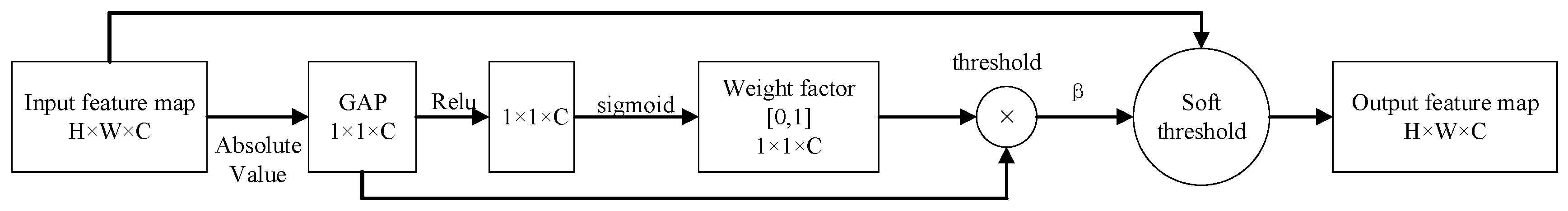
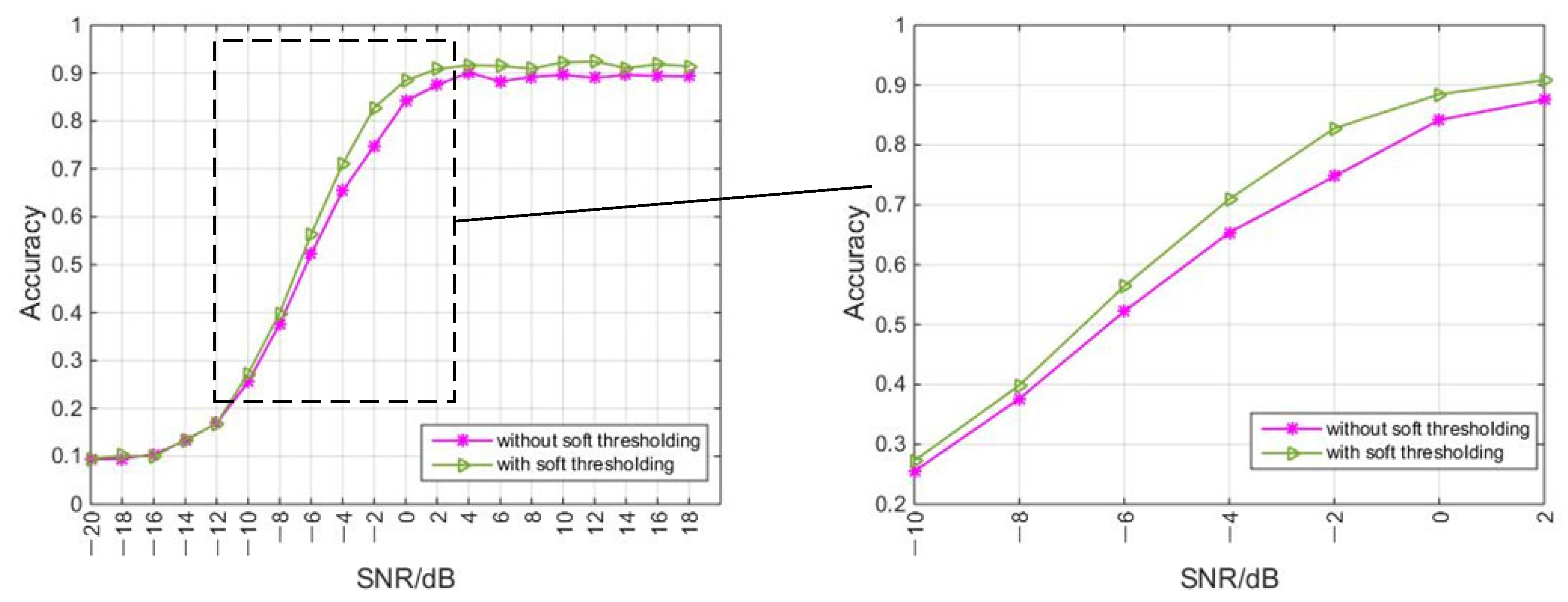
The improved deep residual shrinkage network is added after the CNN, which can generate corresponding thresholds for convolutional feature maps of different channels. Using a soft threshold function to preserve or eliminate convolutional features, the impact of noise-related feature maps on modulation recognition will be reduced to a certain extent, thereby effectively improving recognition accuracy under low SNR conditions.

2. Signal Model and the Proposed Model

2.1. Signal Model

In a single-input single-output communication system, the equivalent baseband signal at the receiving end can be represented as:

$$y[l]=A[l]e^{j(wl+\phi )}x[l]+n[l], l=1,\dots ,L$$

(1)

where $x[l]$ is the modulation signal emitted by the transmitter, $n[l]$ represents the complex Additive White Gaussian Noise (AWGN), $A[l]$ denotes the channel gain, and $w$ and $\phi$ represent frequency offset and phase offset, respectively. $y[l]$ represents the received signal, and $L$ is the number of sampling points for a single signal. The received signals are usually stored in the I/Q form, denoted as $y=[\Re \{y[1]\},\dots ,\Re \{y[L]\};\Im \{y[1]\},\dots ,\Im \{y[L]\}]$, where $\Re \left\{\right\}$ and $\Im \left\{\right\}$ represent the real and imaginary part, respectively.

2.2. Proposed Model

Figure 1 shows the network model proposed in this paper (referred to as PT-DRSN), which mainly consists of a phase transformation layer, CNN, GRU, soft thresholding layer, and a fully connected layer. The phase transformation is used to correct the original I/Q signal and reduce the impact of phase shift. CNN and GRU are used to extract spatial and temporal features of the signal, respectively. It was found that CNN architectures with larger convolutional kernels in early convolutional layers and smaller convolutional kernels in deeper convolutional layers are beneficial for AMR. The two convolutional layers have 75 and 25 convolutional kernel groups, with dimensions of 2 × 8 and 1 × 5, respectively, to ensure the receptive field range and further compress the extracted features. The number of gated recurrent units is 128. The soft thresholding layer is used to process the features obtained by the convolutional layer, eliminate unimportant features below the threshold, and effectively obtain features to improve recognition accuracy.

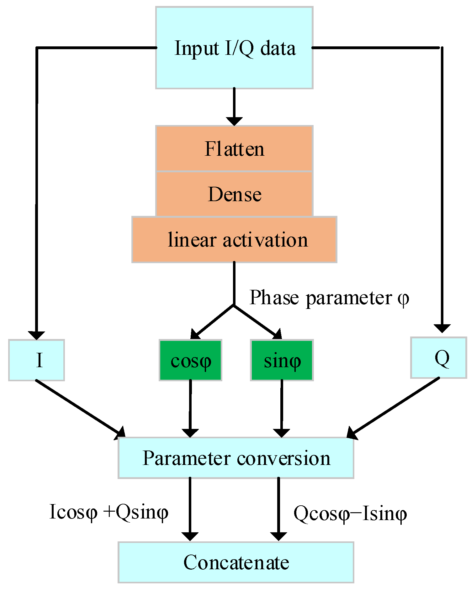
2.2.1. Phase Transformation

As introduced in the signal model, signals are easily affected by channel noise and hardware design during transmission, leading to negative effects including temporal shifting, linear mixing/rotating of the received signal. According to classical signal theory, these adverse effects can be solved through phase transformation [2]. The structure of parameter transformation is shown in Figure 2.

The phase transformation block consists a phase estimator and a parameter transformer. The phase estimator estimates phase parameters by utilizing the principle of phase shift and collaborating with subsequent models for training. Firstly, the original I/Q signal passes through the flattening layer, and its dimension changes from (2128) to (1256), which serves as input to the dense layer. This vector contains rich phase feature information. Finally, an estimated phase parameter $\phi$ is obtained through linear activation. The parameter transformer can realize parametric inverse transformation. The correction mechanism is as follows:

$$\stackrel{\wedge }{y}\left[l\right]=e^{-j\phi }y\left[l\right]=\left[\begin{array}{c}\Re \left\{y[l]\right\}\cos \phi +\Im \left\{y[l]\right\}\sin \phi \\ \Im \left\{y[l]\right\}\cos \phi -\Re \left\{y[l]\right\}\sin \phi \end{array}\right]$$

(2)

where $\phi$ is the estimated phase parameter, and $\stackrel{\wedge }{y}=[\stackrel{\wedge }{y}[1],\dots ,\stackrel{\wedge }{y}[L]]$ is the signal after phase correction.

2.2.2. Soft Thresholding

Soft thresholding is usually used for signal denoising [25,26]. Generally, after processing the original signal, the feature values close to zero are not important, and then the soft threshold function is used to set the features close to zero [24]. The mechanism of soft thresholding is as stated below:

$$z=\left\{\begin{array}{c}x-\tau \\ 0\\ x+\tau \end{array}\right. \begin{array}{c}x>\tau \\ -\tau \le x\le \tau \\ x<-\tau \end{array}$$

(3)

where $x$ is the input feature, $z$ is the output feature, and $\tau$ is a threshold value.

The derivative of soft thresholding can be expressed as follows:

$$\frac{\partial z}{\partial x}=\left\{\begin{array}{c}1\\ 0\\ 1\end{array}\right. \begin{array}{c}x>\tau \\ -\tau \le x\le \tau \\ x<-\tau \end{array}$$

(4)

The derivative value of soft thresholding processing is 1 or 0, which can effectively avoid gradient explosion or vanishing.

To ensure effective denoising of signals, a key task is to retain useful information while converting noise information into features close to zero. Unlike traditional filter designs that require specialized knowledge in signal processing and in which it is difficult to determine an effective threshold suitable for different noise conditions, soft thresholding based on DL can effectively replace the learning filter using gradient descent, avoiding tedious manual operation. Moreover, for signals of different types and SNR, corresponding thresholds can be automatically generated for processing. A mechanism diagram of its action is shown in Figure 3.

The dimensions of the input and output feature maps remain unchanged, with H, W, and C representing the height, width, and number of channels of the feature maps. The processing process is as follows: first, absolute values $x_1$ are taken for all feature maps, and global average pooling (GAP) is performed to obtain a one-dimensional vector. Then, two fully connected layers are used, with the activation functions Relu and sigmoid, to obtain a set of weights $\alpha$ between [0,1]. Multiplying these weights with the global average pooling feature maps can obtain a set of thresholds $\tau$ corresponding to different feature maps, which can be used as the boundary between useful and unimportant features on the corresponding feature maps. By multiplying the threshold and scaling factor $\beta$, the threshold can be adjusted to effectively improve the recognition accuracy. The relevant formulas are expressed as follows:

$$\tau =\alpha \times average(x_1)$$

(5)

$$\tau =\beta \times \tau$$

(6)

3. Dataset and Implementation Details

3.1. Dataset

This paper uses RML2016.10a generated by GNU radio as the dataset. The RML2016.10a dataset includes 11 commonly used modulation signals, including WBFM, AM-DSB, AM-SSB, BPSK, CPFSK, GFSK, 4PAM, 16QAM, 64QAM, QPSK, and 8PSK. The SNR range of each modulation signal is −20~18 dB, with 1000 samples generated every 2 dB interval, resulting in a total of 220,000 modulation signals. Each signal in this dataset has a length of 128, and is stored as a complex group by combining the real part I component and the imaginary part Q component, generated by simulating harsh propagation environments such as Gaussian white noise, multipath fading, sampling rate offset, center frequency offset, etc.

3.2. Implementation Detail

In the experiment, the signals of each modulation style with a single SNR in the dataset were randomly divided into training, validation, and testing sets in a 6:2:2 ratio. The batch size for gradient update is 400. The cross-entropy loss function and Adam optimizer are used. The initial learning rate is 0.001. If the validation loss does not decrease within 10 periods, the callback function is used to halve the learning rate. If the validation loss does not improve within 50 periods, the callback function is used to stop training. All experiments are conducted on a single NVIDIA GeForce GTX1050Ti GPU.

4. Experimental Results and Discussion

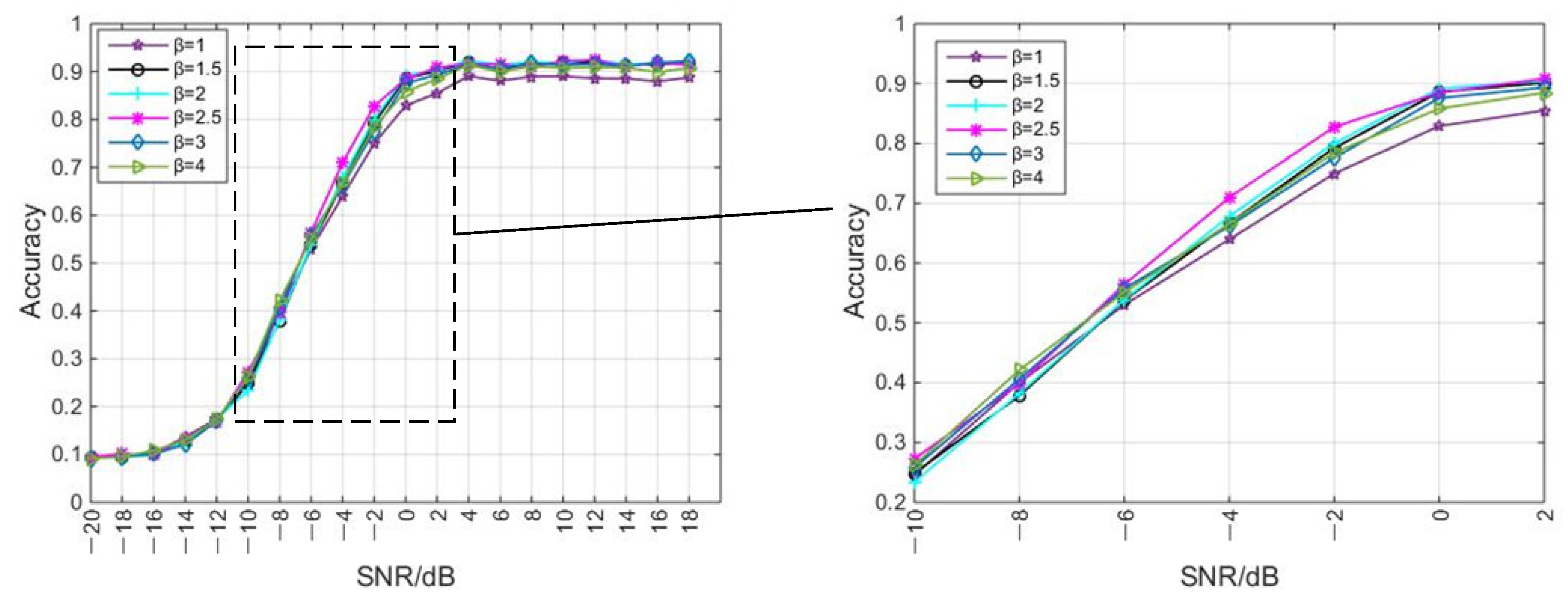
4.1. Scale Factor $\beta$

Using a scaling factor $\beta$ in Formula (6) as an adjustment parameter, which is used to change the threshold, experiments are conducted using different scaling factors, and the recognition accuracy is shown in Figure 4.

From Figure 4, it can be seen that when the scale factor changes from 1 to 2, the recognition accuracy improves. When the scale factor changes from 3 to 4, the recognition accuracy decreases. Overall, when the value of $\beta$ is 2.5, the model has good recognition accuracy at various SNR. An SNR range of −10 dB to 2 dB was selected for observation. Except for the effect at −8 dB, which is at a moderate level, the model is better than the model of other scale factors. The average recognition accuracy of different scale factor models from −20 dB to 18 dB is shown in

Table 1. Average recognition accuracy of models with different scaling factors.

Scale Factor	Average Recognition Accuracy (−20 dB–18 dB)
1	59.69%
1.5	61.65%
2	61.85%
2.5	62.46%
3	61.64%
4	61.40%

.

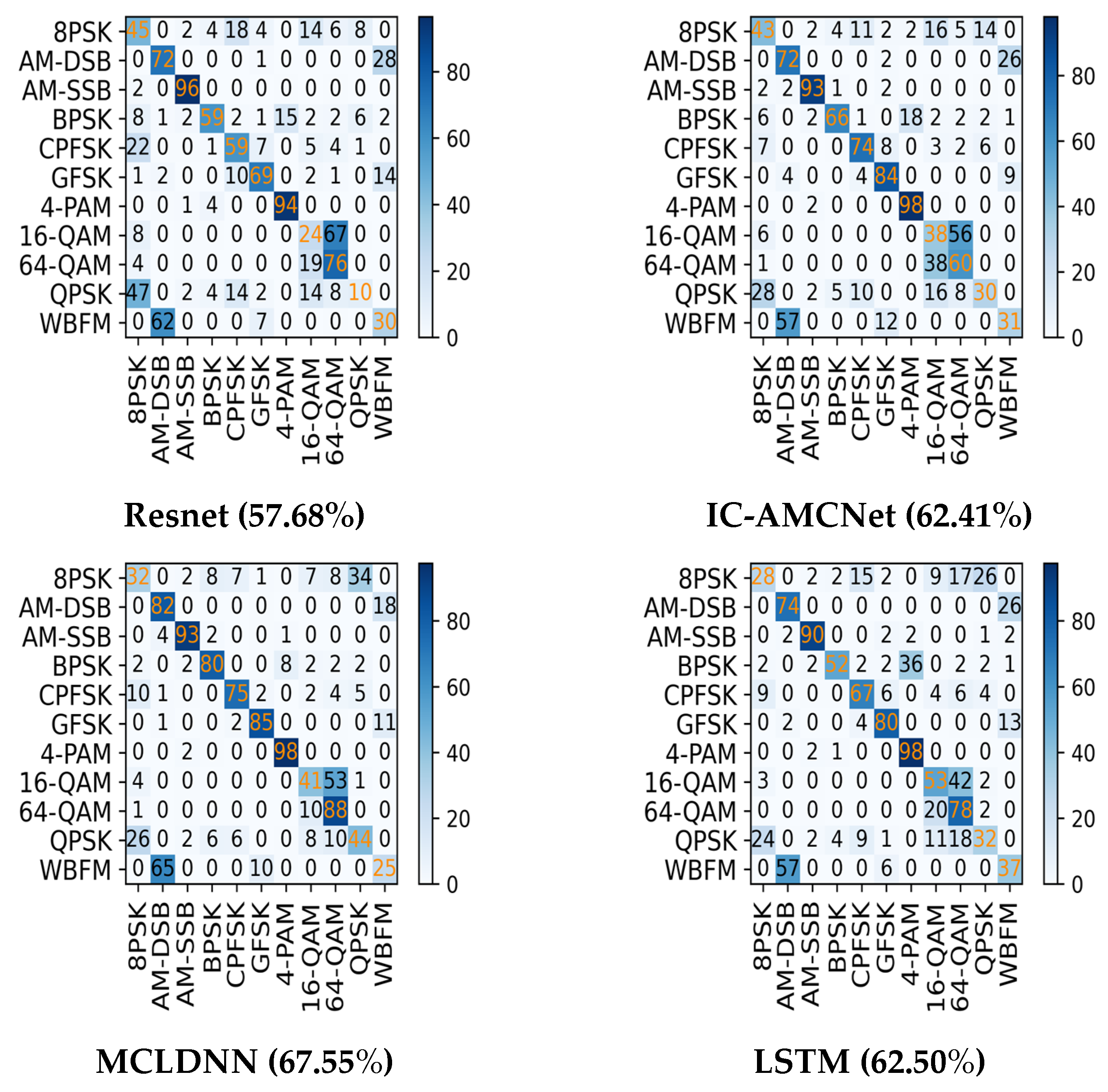
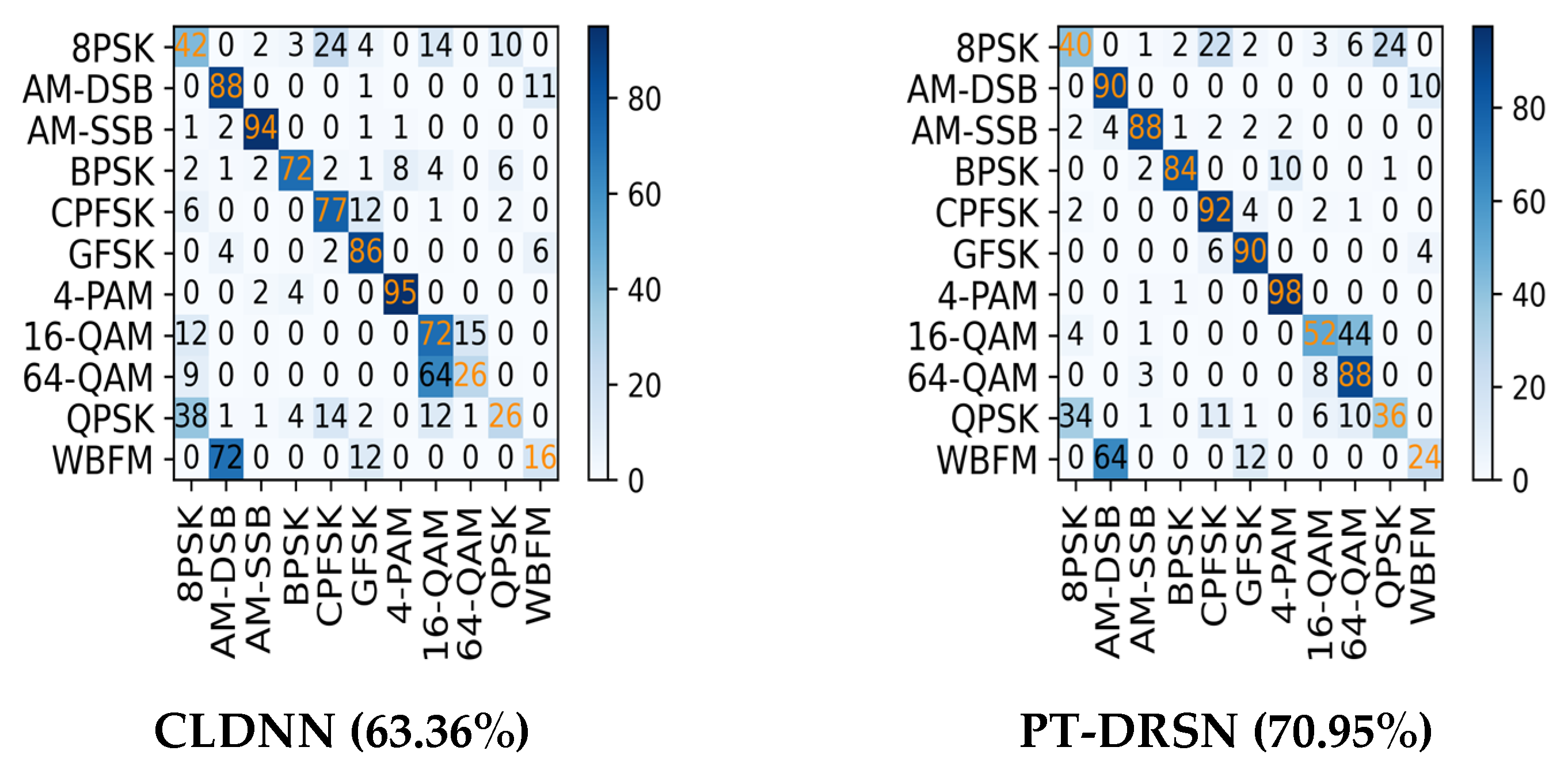
4.2. Recognition Accuracy of Different Models

To testify the superiority of the proposed model, under the same experimental conditions, as shown in Section 3.2, the accuracy of this model is compared with other models: Resnet [14], IC-AMCNet [20], MCLDNN [1], LSTM [21] and CLDNN [14]. The recognition accuracy under various SNR is shown in Figure 5. The average recognition accuracy of each model between −14 dB and −2 dB SNR is shown in

Table 2. Average recognition accuracy of each model between −14 dB and −2 dB.

Model	Resnet	IC-AMCNet	MCLDNN	LSTM	CLDNN	PT-DRSN
Average recognition accuracy ([−14 dB, −2 dB])	35.83%	37.86%	41.51%	39.57%	38.44%	43.93%

.

From Figure 5, it can be seen that the recognition accuracy of the proposed model PT-DRSN is better than other models when the SNR is from −14 dB to −2 dB. Combined with Table 2, the average recognition accuracy has improved by 2.4% to 8% in this SNR. When the SNR is higher than 0 dB, it is not on par with the recognition accuracy of the model MCLDNN. However, the model MCLDNN is complex, has multiple parameters, and requires a long training time. The next section will make specific comparisons. Overall, the model proposed in this paper outperforms other models. It can be concluded that the combination of phase transformation and improved deep residual shrinkage network proposed in this paper is effective for signal denoising at low SNR.

To visually demonstrate the superiority of the model PT-DRSN in AMR under low SNR, Figure 6 shows the identification confusion matrices of different models at a SNR of −4 dB.

From the confusion matrix diagram, it can be seen that the recognition accuracy of the model PT-DRSN is higher and the error rate is lower. Analyzing the factors that affect the accuracy of the model PT-DRSN, the main recognition errors are between 16QAM and 64QAM, as well as between AM-DSB and WBFM. A possible factor is that 16QAM and 64QAM are confused due to the presence of a large number of overlapping constellation points in the digital domain. AM-DSB and WBFM are both continuously modulated and generated through analog audio signals, and their features tend to be consistent in the complex plane.

4.3. Model Complexity

We compare the complexity of the models involved in training on the benchmark dataset RadioML2016.10A, and the specific parameters are shown in

Table 3. Model complexity comparison.

Model	Parameters	Training Time (per Epoch)
Resnet	3,098,283	91 s
IC-AMCNet	1,264,011	19 s
MCLDNN	406,199	51 s
LSTM	201,099	30 s
CLDNN	517,643	64 s
PT-DRSN	84,571	20 s

.

From Table 3, it can be seen that the model PT-DRSN has a small number of parameters, reduced by 79% and 57% compared to models MCLDNN and LSTM, and a shorter single cycle training time. Compared to models MCLDNN and LSTM, it has shortened by 61% and 33%, and is slightly longer than model IC-AMCNet. This is because model IC-AMCNet does not have a recurrent neural network module, and the time feature extraction of modulated signals is not sufficient. Simply relying on convolutional neural networks to extract spatial features for modulation recognition results in a large number of parameters and low recognition accuracy. The proposed model combines spatial and temporal feature extraction, and overall performance is superior to other models.

4.4. Module Effectiveness

This paper proposes a soft thresholding module for convolutional features based on the deep residual shrinkage network. To quantify the effectiveness of the soft thresholding module, this section mainly compares the experimental parameters of the model with and without this module. The recognition accuracy is shown in Figure 7, and detailed parameters are presented in

Table 4. Model parameter comparison (with and without soft thresholding).

Model	Parameters	Training Time (per Epoch)	Average Recognition Accuracy
			(−20 dB–18 dB)	(−10 dB–2 dB)
With soft thresholding	84,571	20 s	62.46%	65.22%
Without soft thresholding	71,871	16	60.05%	61.02%

.

From Figure 7, it can be found that the soft thresholding module of the model is effective in improving recognition accuracy, especially when the SNR is from −10 dB to 2 dB, that is, under low SNR conditions, the recognition accuracy is improved by 1.77% to 8.04%. As shown in Table 4, the addition of a soft thresholding module to the model does not change much in the number of parameters. At the expense of a certain training time, the average recognition accuracy of the full SNR is improved by 2.41%. In the SNR range of from −10 dB to 2 dB, the average recognition accuracy is improved by 4.20%. Overall, it can be seen that the soft thresholding module is effective in improving modulation recognition accuracy, especially under low SNR conditions.

5. Conclusions

This paper proposes an efficient AMR model based on phase transformation and deep residual shrinkage network. Firstly, the raw I/Q signal is used as input to avoid the problem of low real-time performance caused by signal preprocessing. Then, spatial and temporal features are extracted separately through CNN and GRU. Phase transformation and soft thresholding are used to denoise the signal. The experiment shows that the proposed model effectually improves the modulation recognition accuracy under low SNR, and the model has a small number of parameters and relatively short training time. However, this paper only considers the threshold on the convolutional channel dimension, distinguishing between signals and noise through the processing of convolutional feature values, but ignoring the spatial distribution of noise. Therefore, this denoising method is not comprehensive enough and needs further improvement. In future research, signal denoising will be based on DL to integrate channel and spatial dimensions, thereby further improving the recognition accuracy of low SNR.

References

1. Xu, J.; Luo, C.; Parr, G.; Luo, Y. A Spatiotemporal Multi-Channel Learning Framework for Automatic Modulation Recognition. IEEE Wirel. Commun. Lett. 2020, 9, 1629–1632. [Google Scholar] [CrossRef]
2. Zhang, F.; Luo, C.; Xu, J.; Luo, Y. An Efficient Deep Learning Model for Automatic Modulation Recognition Based on Parameter Estimation and Transformation. IEEE Commun. Lett. 2021, 25, 3287–3290. [Google Scholar] [CrossRef]
3. Xu, J.L.; Su, W.; Zhou, M. Likelihood-Ratio Approaches to Automatic Modulation Classification. IEEE Trans. Syst. Man Cybern. Part C (Appl. Rev.) 2011, 41, 455–469. [Google Scholar] [CrossRef]
4. Wei, W.; Mendel, J.M. Maximum-Likelihood Classification for Digital Amplitude-Phase Modulations. IEEE Trans. Commun. 2000, 48, 189–193. [Google Scholar] [CrossRef]
5. Dulek, B. Online Hybrid Likelihood Based Modulation Classification Using Multiple Sensors. IEEE Trans. Wirel. Commun. 2017, 16, 4984–5000. [Google Scholar] [CrossRef]
6. Hazza, A.; Shoaib, M.; Alshebeili, S.A.; Fahad, A. An Overview of Feature-Based Methods for Digital Modulation Classification. In Proceedings of the 2013 1st International Conference on Communications, Signal Processing, and Their Applications (ICCSPA), Sharjah, United Arab Emirates, 12–14 February 2013; pp. 1–6. [Google Scholar]
7. Chan, Y.; Gadbois, L.; Yansouni, P. Identification of the Modulation Type of a Signal. In Proceedings of the ICASSP ’85, IEEE International Conference on Acoustics, Speech, and Signal Processing, Tampa, FL, USA, 26–29 April 1985; Volume 10, pp. 838–841. [Google Scholar]
8. Hong, L.; Ho, K.C. Identification of Digital Modulation Types Using the Wavelet Transform. In Proceedings of the MILCOM 1999, IEEE Military Communications, Conference Proceedings (Cat. No.99CH36341), Atlantic City, NJ, USA, 31 October–3 November 1999; Volume 1, pp. 427–431. [Google Scholar]
9. Swami, A.; Sadler, B.M. Hierarchical Digital Modulation Classification Using Cumulants. IEEE Trans. Commun. 2000, 48, 416–429. [Google Scholar] [CrossRef]
10. Nandi, A.K.; Azzouz, E.E. Algorithms for Automatic Modulation Recognition of Communication Signals. IEEE Trans. Commun. 1998, 46, 431–436. [Google Scholar] [CrossRef]
11. Zhang, X.; Sun, J.; Zhang, X. Automatic Modulation Classification Based on Novel Feature Extraction Algorithms. IEEE Access 2020, 8, 16362–16371. [Google Scholar] [CrossRef]
12. Jiang, Y.; Zhang, Z.-Y.; Qiu, P.-L. Modulation Classification of Communication Signals. In Proceedings of the IEEE MILCOM 2004, Military Communications Conference, Monterey, CA, USA, 31 October–3 November 2004; Volume 3, pp. 1470–1476. [Google Scholar]
13. O’Shea, T.J.; Corgan, J.; Clancy, T.C. Convolutional Radio Modulation Recognition Networks. In Proceedings of the Engineering Applications of Neural Networks, EANN 2016; Jayne, C., Iliadis, L., Eds.; Springer International Publishing AG: Cham, Switzerland, 2016; Volume 629, pp. 213–226. [Google Scholar]
14. Liu, X.; Yang, D.; Gamal, A.E. Deep Neural Network Architectures for Modulation Classification. In Proceedings of the 2017 51st Asilomar Conference on Signals, Systems, and Computers, Pacific Grove, CA, USA, 29 October–1 November 2017; pp. 915–919. [Google Scholar]
15. Zeng, Y.; Zhang, M.; Han, F.; Gong, Y.; Zhang, J. Spectrum Analysis and Convolutional Neural Network for Automatic Modulation Recognition. IEEE Wirel. Commun. Lett. 2019, 8, 929–932. [Google Scholar] [CrossRef]
16. Peng, S.; Jiang, H.; Wang, H.; Alwageed, H.; Zhou, Y.; Sebdani, M.M.; Yao, Y.-D. Modulation Classification Based on Signal Constellation Diagrams and Deep Learning. IEEE Trans. Neural Netw. Learn. Syst. 2019, 30, 718–727. [Google Scholar] [CrossRef] [PubMed]
17. He, P.; Zhang, Y.; Yang, X.; Xiao, X.; Wang, H.; Zhang, R. Deep Learning-Based Modulation Recognition for Low Signal-to-Noise Ratio Environments. Electronics 2022, 11, 4026. [Google Scholar] [CrossRef]
18. Wang, Y.; Guo, L.; Zhao, Y.; Yang, J.; Adebisi, B.; Gacanin, H.; Gui, G. Distributed Learning for Automatic Modulation Classification in Edge Devices. IEEE Wirel. Commun. Lett. 2020, 9, 2177–2181. [Google Scholar] [CrossRef]
19. Cheng, Q.; Wang, H.; Zhu, B.; Shi, Y.; Xie, B. A Real-Time UAV Target Detection Algorithm Based on Edge Computing. Drones 2023, 7, 95. [Google Scholar] [CrossRef]
20. Hermawan, A.P.; Ginanjar, R.R.; Kim, D.-S.; Lee, J.-M. CNN-Based Automatic Modulation Classification for Beyond 5G Communications. IEEE Commun. Lett. 2020, 24, 1038–1041. [Google Scholar] [CrossRef]
21. Rajendran, S.; Meert, W.; Giustiniano, D.; Lenders, V.; Pollin, S. Deep Learning Models for Wireless Signal Classification With Distributed Low-Cost Spectrum Sensors. IEEE Trans. Cogn. Commun. Netw. 2018, 4, 433–445. [Google Scholar] [CrossRef]
22. Njoku, J.N.; Morocho-Cayamcela, M.E.; Lim, W. CGDNet: Efficient Hybrid Deep Learning Model for Robust Automatic Modulation Recognition. IEEE Netw. Lett. 2021, 3, 47–51. [Google Scholar] [CrossRef]
23. Xu, Z.; Hou, S.; Fang, S.; Hu, H.; Ma, Z. A Novel Complex-Valued Hybrid Neural Network for Automatic Modulation Classification. Electronics 2023, 12, 4380. [Google Scholar] [CrossRef]
24. Zhao, M.; Zhong, S.; Fu, X.; Tang, B.; Pecht, M. Deep Residual Shrinkage Networks for Fault Diagnosis. IEEE Trans. Ind. Inf. 2020, 16, 4681–4690. [Google Scholar] [CrossRef]
25. Donoho, D.L. De-Noising by Soft-Thresholding. IEEE Trans. Inf. Theory 1995, 41, 613–627. [Google Scholar] [CrossRef]
26. Isogawa, K.; Ida, T.; Shiodera, T.; Takeguchi, T. Deep Shrinkage Convolutional Neural Network for Adaptive Noise Reduction. IEEE Signal Process. Lett. 2018, 25, 224–228. [Google Scholar] [CrossRef]
Figure 1. The structure of the proposed PT-DRSN.
Electronics 13 02141 g001
Figure 2. The structure of phase transformation.
Electronics 13 02141 g002
Figure 3. The structure of soft thresholding.
Electronics 13 02141 g003
Figure 4. Recognition accuracy under different scaling factors.
Electronics 13 02141 g004
Figure 5. Recognition accuracy of different models.
Electronics 13 02141 g005
Figure 6. Identification confusion matrix for different models at −4 dB.
Electronics 13 02141 g006aElectronics 13 02141 g006b
Figure 7. Comparison of model recognition accuracy (with and without soft thresholding).
Electronics 13 02141 g007