Article

Fast Versatile Video Coding (VVC) Intra Coding for Power-Constrained Applications

1
College of Compute, National University of Defense Technology, Changsha 410073, China
2
Center for Strategic Studies, Chinese Academy of Engineering, Beijing 100088, China
3
Department of Electronic Engineering, Tsinghua University, Beijing 100084, China
4
China Mobile (Hangzhou) Information Technology Company, Ltd., Hangzhou 310000, China
5
Faculty of Information Technology, Beijing University of Technology, Beijing 100124, China
6
China Telecom Research Institute, Shanghai 200122, China
7
School of Communications and Information Engineering, Chongqing University of Posts and Telecommunications, Chongqing 400065, China
*
Author to whom correspondence should be addressed.
Electronics 2024, 13(11), 2150; https://doi.org/10.3390/electronics13112150
Submission received: 8 March 2024 / Revised: 24 May 2024 / Accepted: 29 May 2024 / Published: 31 May 2024

Abstract

:
Versatile Video Coding (VVC) achieves impressive coding gain improvement (about 40%+) over the preceding High-Efficiency Video Coding (HEVC) technology at the cost of extremely high computational complexity. Such an extremely high complexity increase is a great challenge for power-constrained applications, such as Internet of video things. In the case of intra coding, VVC utilizes the brute-force recursive search for both the partition structure of the coding unit (CU), which is based on the quadtree with nested multi-type tree (QTMT), and 67 intra prediction modes, compared to 35 in HEVC. As a result, we offer optimization strategies for CU partition decision and intra coding modes to lessen the computational overhead. Regarding the high complexity of the CU partition process, first, CUs are categorized as simple, fuzzy, and complex based on their texture characteristics. Then, we train two random forest classifiers to speed up the RDO-based brute-force recursive search process. One of the classifiers directly predicts the optimal partition modes for simple and complex CUs, while another classifier determines the early termination of the partition process for fuzzy CUs. Meanwhile, to reduce the complexity of intra mode prediction, a fast hierarchical intra mode search method is designed based on the texture features of CUs, including texture complexity, texture direction, and texture context information. Extensive experimental findings demonstrate that the proposed approach reduces complexity by up to 77% compared to the latest VVC reference software (VTM-23.1). Additionally, an average coding time saving of 70% is achieved with only a 1.65% increase in BDBR. Furthermore, when compared to state-of-the-art methods, the proposed method also achieves the largest time saving with comparable BDBR loss. These findings indicate that our method is superior to other up-to-date methods in terms of lowering VVC intra coding complexity, which provides an elective solution for power-constrained applications.

1. Introduction

As the next generation of the video coding standard, Versatile Video Coding (VVC) [1] has been developed by the Joint Video Exploration Team of the ITU-T Video Coding Group and the ISO/IEC Moving Picture Experts Group. The purpose of VVC standard is to provide adequate coding gain enhancement over the High Efficiency Video Coding (HEVC) standard to meet the requirements of the future video market, such as 4 K/8 K ultra-high definition, high dynamic range, virtual reality, and 360 degree video content. According to reports, the VVC reference software (VTM) achieves a 45% bitrate reduction when compared to HEVC (HM) under standard test settings [2]. In fact, the coding efficiency improvement mainly benefits from several newly adopted innovative video coding techniques (e.g., the quadtree with nested multi-type tree (QTMT) partition structure [3], 65 directional intra prediction modes, and affine motion compensated prediction [4]), which leads to an extremely high encoding complexity increase. Based on the AHG report, the intra coding complexity of VTM increases more than 10 times over that of HM under the All-Intra test configuration [5]. However, such a high computational complexity will bring a significant challenge for power-constrained applications, such as Internet of video things (IoVT) [6]. The substantial volume of data also poses potential risk for IoVT security. Especially in terms of real-time requirements, more rapid video encoding and decoding is desired. Consequently, fast coding algorithms of VVC must be developed in order to decrease the computing complexity.
Brute-force recursive RDO searches of intra prediction modes and the partition structure of CU occupy most of the time in VVC intra coding. VVC adopts the QTMT partition structure to make CU partition shapes more flexible as shown in Figure 1. A quadtree (QT) is first used to partition a coding tree unit (CTU), and then each leaf node is partitioned by a multi-type (MT) structure until the size of the CU is the smallest. Vertical binary tree (BV), horizontal binary tree (BH), vertical ternary tree (TV), and horizontal ternary tree (TH) are four partition options of a multi-type tree (MT) structure. A QTMT partition structure is depicted in Figure 1, where different lines indicate different partition modes. Indeed, the QTMT coding block structure better suits the characteristics of various texture patterns, resulting in significant coding efficiency gain. However, such an impressive performance improvement comes at the expense of extremely high computational complexity. Based on the principle of the QTMT structure with several limitations, it can be deduced that there are, in total, more than 30,000 possible CU partition modes for a 128 × 128 CTU. With so many Rate-Distortion Optimization (RDO) based brute-force recursive searches, they contribute to the largest proportion of the encoding time.Therefore, a central priority is to achieve an efficient CU partition method for the fast coding algorithm.
In addition, to further reduce the spatial redundancy of the intra frames, VVC designs up to 67 intra prediction modes, whereas HEVC only allows for 35. Meanwhile, several advanced prediction techniques are also proposed to further improve the intra coding efficiency, such as matrix weighted intra prediction [7], multi-reference line intra prediction [8], and intra sub-partition [9]. Evidently, the improvement of the VVC intra coding efficiency beyond HEVC requires more calculations. Therefore, instead of conducting the brute-force traversal of the expensive RDO process for all 67 modes as shown in Figure 2, the classical three-step fast intra mode decision (TS-FMD) [10] of HEVC is inherited by VVC to reduce the computational complexity of the intra mode prediction. First, VVC adopts rough mode decision (RMD) [11] to limit the number of modes for the RDO search process. In RMD, N (usually 2 or 3) modes with the smallest Hadamard transform-based (HAD) cost are chosen from the original 35 modes of HEVC to construct a candidate list. The HAD cost is calculated as follows:
H A D C o s t = S A T D + λ · B i t M o d e
where S A T D is the sum of residual signal’s absolute Hadamard transformed differences, λ represents the Lagrange multiplier, and B i t M o d e specifies the number of bits for encoding the intra mode information. Second, two kinds of intra mode are integrated to create a final candidate list consisting of two neighbors (left and right) of the N RMD modes and a most probable model (MPM) generated by the neighboring CUs. Finally, two or three models from the candidate list with minimal HAD-cost proceed through the RDO process to generate the final intra prediction mode. The RD-cost for each mode is calculated as follows:
R D C o s t = S S E + λ · B i t T o t a l
where S S E is the sum of squared errors between the original and reconstructed CU, and B i t T o t a l is the bits budget to encode the selected mode. It can be seen that TS-FMD selects the best mode with about 40 times of the RMD process and 2 or 3 times of the RDO process. The TS-FMD approach can reduce the complexity of the intra prediction processing to some extent but requires additional reduction in the computing complexity.
To minimize the computational cost of VVC significantly, we propose a fast intra coding algorithm that integrates a more efficient CU partition strategy and a fast intra mode prediction scheme. First, a detailed statistical analysis for the CU depth distribution and intra prediction mode is presented, which motivates us to design the fast intra coding algorithm. From the distribution of the CU depth, the RDO brute-force recursive search of the CU partition process is sped up by using random forest-based classification. The CUs are categorized as simple, fuzzy, and complex CUs based on their texture characteristics. One random forest classifier predicts the best partition modes of simple and complicated CUs directly, while another random forest identifies the early termination of the partition process for fuzzy CUs. This approach not only maximizes the potential for speed improvement but also effectively mitigates bitrate distortion (BDBR) losses, particularly for fuzzy CUs. Meanwhile, a fast hierarchical intra mode search method based on the CU texture feature is presented, and experimental results prove that our method significantly lessens the computational cost of intra mode prediction while causing negligible RD loss.
The remainder of this paper is structured as follows. Section 2 provides an overview of the related work. The statistical distribution of intra prediction and CU depth is explored in Section 3. Section 4 describes our algorithm in details. The extensive experimental results and several ablation studies are shown in Section 5, while Section 6 ends with a conclusion.

2. Related Works

The fast intra coding algorithm focuses on two main tasks, the fast CU partition mode decision and fast intra mode prediction, respectively.

2.1. Fast CU Partition Structure Decision

For the CU partition structure decision, there are three kinds of strategies, including early termination, multi-classification, and joint classification. The early-termination policy attempts to determine whether the recursive CU partition terminates after partitioning at the current depth level. It is easy to understand that the early termination mainly happens in the region of smooth texture. It maintains the RD performance well, but the reduction in computational complexity is also limited. The multi-classification strategy designs a sophisticated prediction model to directly obtain the optimal partition mode. It reduces the computational complexity significantly. However, the complex partition structure of VVC leads to the limitation of prediction accuracy and greater loss of RD performance. For the sake of improving the prediction accuracy while achieving a large amount of time saving, joint classification is designed to predict the probability of each partition mode, and one or more partition modes with highest probability are selected as the candidates of the final encoding mode.
For each of the above three strategies, three categories of common methods are used, including heuristic methods, traditional machine learning methods, and end-to-end deep learning methods. The heuristic methods first extract some handcrafted features in the encoding process (e.g., image texture complexity, rate-distortion cost, and context information), and the decision criteria are based on the preset thresholds. Its efficiency is influenced by the chosen features and decision criteria simultaneously. The greatest advantage of heuristic methods is that they are very simple but accuracy is limited. Traditional machine learning methods employ advanced classifier (e.g., decision tree) to automatically learn a decision function instead of manually designing one of the heuristic methods. However, it still needs to select some handcrafted features. On the contrary, end-to-end deep learning methods attempt to accomplish the feature extraction and decision work automatically with advanced deep neural networks.

2.1.1. Heuristic Methods

In the last few years, several heuristic methods have extensively been adopted for the fast CU partition structure decision algorithms in HEVC and VVC. By considering the spatial correlation, Gu et al. used context information to skip some CU depths that are rarely found in neighboring CUs [12]. Li et al. proposed an early intra CU size decision approach for VVC based on a configurable decision model [13]. Ni et al. proposed a texture analysis-based TT and BT partition strategy with the gradient-based intra mode decision to accelerate VVC intra coding [14]. In [15], the Bayesian decision rule was used to design an early termination framework for CU partition based on the distribution of partition modes and RD cost. Similarly, an early termination strategy based on the HAD and RD cost was presented in [16]. Saldanha et al. proposed to remove abundant predictions by analyzing the characteristics of current block and encoding context using selected intra prediction modes [17]. In [18], Cui et al. predicted the likelihood of partition modes according to the directional gradient, and then eliminated the unlikely partitions. Fan et al. suggested that if the texture of the current CU was found to be smooth, CU partition would be terminated. Then, the gradient could be utilized to determine whether or not to split the CU by QT partition. Finally, one QTMT partition would be selected based on the difference of the variance of the sub-CUs [19].

2.1.2. Machine Learning Methods

Since CU partition can be regarded as a classification problem, both VVC and HEVC employ machine learning. Kim et al. suggested a fast CU partition approach based on Bayesian decision making that predicts whether the CU partition should be terminated via offline and online joint learning [20]. Wang et al. proposed a fast CU decision algorithm based on FSVMs and DAG-SVMs for coding complexity reduction, which divides the CU-partitioning process into two stages and symmetrically extracts some of the same CU features [21]. The fast CU size decision method was guided by the SVM classification of the complexity degree [22]. Erabadda et al. devised a weighted SVM-based CU size selection algorithm [23]. This algorithm extracts texture complexity, RD cost and context information to train the model. Shan et al. proposed a fast CU partition algorithm based on SVM and the Laplace Transparent Composite Model (LPTCM) [24]. To obtain the partition mode, the feature vectors called the Summation of Binarized Outlier Coefficient are recovered from the original frames using LPTCM and fed to the online trained SVM. The decision tree-based fast CTU partition structure in [25] explores the distribution of CU depths and designs a joint-classification framework to predict the partition probability for each partition mode. Zhang et al. designed an individual fast CU partition scheme for different CU types based on their texture complexity, while the CU with simple texture complexity was not handled efficiently [26].

2.1.3. Deep Learning Methods

Benefiting from the development of deep learning, end-to-end prediction of CU partition modes have been developed to lessen the computational complexity of video coding recently. Wu et al. proposed a hierarchical grid fully convolutional network to predict the QTMT partition structure for fast VVC intra coding [27]. Chen et al. proposed to predict CU partition modes for VVC intra coding by a CNN model, which is trained with the neighboring line pixels and quantization parameters [28]. In [29], heuristic and deep learning methods were combined. A threshold-based texture classification model was first conducted to terminate the partition process of the homogeneous CUs. Then, three different CNNs were designed to predict the partition modes for the remaining CUs. In [30], a bagged tree model was employed to predict the splitting of a CTU, and the partition problem of a 32 × 32 -sized CU was modeled as a 17-output classification task. Wang et al. [31] proposed a densely connected convolution neural network to predict the partition of coding units (CUs), which significantly reduces the coding complexity. Zan et al. proposed a redesigned U-NET with a quality parameter fusion network to accelerate the QTMT partition process [32]. Tang et al. proposed an adaptive CU partition choice with a pooling-variable CNN architecture, which is applicable to a wide range of CU sizes and requires only one parameter set to be configured [33]. In [34], a CNN was built for each 64 × 64 CU to predict a probability vector to speed up the partition process during encoding.

2.2. Fast Intra Mode Prediction

Based on the discovery that intra mode prediction is highly associated to texture features, the fast intra mode prediction algorithms focus on modeling such a relationship to accelerate the intra mode prediction process. Each block had five different edge directions, determined in [35]. A limited set of intra modes was defined for the specified edge type, reducing the complexity of the RMD process. In [36], a gradient-based strategy was presented to decrease the number of RMD and RDO candidate modes: the average gradients in the horizontal (AGH) and vertical (AGV) directions were utilized to determine the rough range of the block direction; the number of RMD and RDO modes was reduced based on the values of AGH, AGV, and AGH/AGV. In addition, Zhang et al. also proposed a gradient-based method to eliminate irrelevant orientation modes from the candidate list [37]. In order to further reduce the complexity, a mode classification based on texture features was developed to adaptively reduce the number of intra modes in chrominance. Jamali et al. not only utilized the Prewitt operator in the gradient but also tried to skip needless modes by predicting the cost of RDO [38]. In [39], progressive rough mode search (pRMS) was conducted based on the HAD cost, selecting potential modes rather than traversing all candidates. In the subsequent RDO process, fewer candidate modes were selected by pRMS. Jamali et al. succeeded in rejecting non-promising modes from further processing by utilizing the prediction modes and saving significant computations [40]. Ogata et al. [41] offered a fast intra mode decision that limits the number of possible modes by using DCT coefficients and outliers from nearby blocks.
In addition, machine learning and deep learning were also applied for intra mode prediction. Ryu et al. designed a random forest which uses four pixel points as features to reduce the number of candidates before optimizing rate-distortion [42]. Song et al. offered a fast intra mode prediction algorithm based on CNN which outputs the probability of each mode being selected as the optimal mode [43]. Meanwhile, a corner detection algorithm was developed to further minimize the number of candidate modes entering the RDO process. Ting et al. used an improved LeNet-5 CNN model to predict the probability of each mode, which achieved higher prediction accuracy [44].

3. Statistical Analysis of Intra Coding

The statistical study of VVC intra coding is useful for proposing and comprehending novel algorithms. The following study employs 26 JCT-VC test sequences encoded with VTM7.0 and placed in an all-intra configuration. These test sequences range from Class A1 to Class F with varying resolutions and contents.

3.1. CU Partition Depth Distribution

Similar to [26], the CU depth distribution of different sequences with Q P s { 22 , 27 , 32 , 37 } is shown in Table 1. It should be noted that only one sequence of each class is analyzed based on VTM 2.0 in [26]. However, our analysis is based on all of the sequences of each class. In addition, our experiments are implemented with VTM 7.0, which includes some new advanced intra coding techniques as compared to VTM 2.0. The results are the average values for each class. D i , j denotes the CU depth with QT depth of i , i { 1 , 2 , 3 , 4 } and MT depth of j , j { 1 , 2 , 3 } . There are some statistical conclusions that can be observed from Table 1 as follows:
(1)
High-resolution sequences tend to be coded with a large CU size, and lower-resolution sequences prefer using a small CU size.
(2)
The percentage of large size CU increases gradually with the increasing of QP.
(3)
The percentage of CUs decreases with the decreasing of the CU size on the trend.
(4)
Nearly two thirds of regions are coded with MT CUs.
In addition, some intuitive observations between the texture complexity and CU partition mode can be found in Figure 3 as follows:
(1)
Generally, flat regions imply a simple CU partition mode, while rich texture regions adopt a more complex CU partition structure.
(2)
Since two directions of multi-type tree partition are employed in VVC, the partition direction is related to the texture direction. Taking the edge areas as an example, the texture extends vertically with the woman’s body, and thus the majority of partitions tend to be vertical as well.
(3)
If the texture complexity among the sub-CUs is different, the current CU probably needs to be split into smaller CUs.
Furthermore, statistical analysis of the relationship between the texture complexity and CU partition mode is performed as follows. The variance of a CU is defined as its texture complexity. As shown in Figure 4, by comparing the texture complexity of the current CU and its neighboring CUs, we classify CUs into three categories. If the texture complexity of the current CU is smaller than the minimum texture complexity of its neighboring CUs, it is classified as a simple CU; if the texture complexity of the current CU is greater than the maximum value of its neighboring CUs, it is classified as a complex CU. Otherwise, it is classified as a fuzzy CU. The partition probability of the three CU categories is shown in Table 2:
(1)
Nearly two-thirds of the complex CUs need to be further partitioned, especially for the videos with lower resolution.
(2)
More than 70% of simple CUs terminate the partition process at the current depth level, especially for the videos with high resolution.
(3)
The probability of early termination for fuzzy CUs is about 50%.
It seems that the partition process for complex and simple CUs has an obvious tendency, while the partition for fuzzy CUs is ambiguous. Therefore, we propose different acceleration schemes for the three categories of CUs, respectively.

3.2. Intra Prediction Mode Distribution

The 67 intra prediction modes of VVC can be divided into DC mode, planar mode, and angle mode. The distribution of the intra mode is presented in Table 3, and some observations can be obtained as follows:
(1)
Intra mode distribution is closely related to the sequence resolution. High-resolution sequences have more flat areas, which tend to select DC or planar mode as the best mode.
(2)
About 78.6% of the CUs best mode can be found in MPM, and it reaches 85% for some sequences with a high spatial correlation.
To lessen the computational cost of intra mode prediction, a feasible way is to narrow down the candidate list by removing some improbable modes. According to the first conclusion, the CUs can first be divided into two types, one is a flat CU and the other one is a non-flat CU. For flat CU, only DC and planar modes are checked to obtain the best mode. This method reduces the complexity to a certain extent, but there are still more than 60% of CUs that select directional modes.
Intuitively, the intra prediction direction is inextricably related to the texture direction. For example, as shown in Figure 5, the texture direction is 135° diagonal. The optimal intra prediction direction is more likely corresponding to it. The opposite direction of the texture direction is nearly impossible to be chosen as the optimal intra modes. It inspires us that the complexity reduction benefits from eliminating modes in unnecessary directions. The gradient is adopted to reflect the texture direction. As shown in Figure 5, it is clear that the texture direction (135° diagonal) has the smallest gradient value. By contrast, the opposite direction of the texture direction (45° diagonal) is almost impossible to be selected as the intra prediction direction, which has the largest gradient value. We investigate the probability that CUs choose the modes located in the direction with the biggest gradient value, which is shown in Table 4 and it can be found that no more than 10% of CUs select the modes in the direction with the biggest gradient value.

4. Proposed Algorithm

Based on the above analysis of the statistical results in Section 3, an efficient fast algorithm for VVC intra coding is proposed, which is composed of random forest-guided classification for fast CU partition and hierarchical search-based fast intra mode prediction.

4.1. Random Forest-Guided Classification for Fast CU Partition

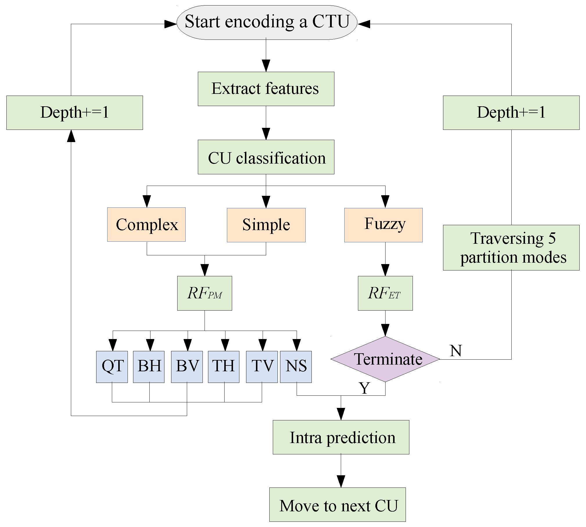
4.1.1. System Overview of CU Partition Structure

The proposed fast CU partition algorithm uses the random forest classifier to deal with different kinds of CU. By comparing the texture complexity between neighboring CUs, we classify CUs into three categories: simple, complex, and fuzzy. To find the best partition mode for simple and complex CUs, we utilize the same trained random forest classifier. Another random forest is utilized for fuzzy CU to decide if the partition process terminates. The overall structure is shown in Figure 6.

4.1.2. Feature Extraction

In addition to texture complexity, four other features related to the partition mode will be analyzed, including gradient information, the sub-CUs complexity difference, context information, and block information.
Texture complexity: Variance can be used to describe texture complexity as follows:
V a r = 1 W · H x = 1 W y = 1 H ( P ( x , y ) M e a n ) 2
M e a n = 1 W · H x = 1 W y = 1 H P ( x , y )
where W is the width of target CU, H is the height of target CU, and P ( x , y ) is the pixel value at position (x,y).
However, the two pictures shown in Figure 7 have the same variance but different textures, which leads to a different partition. It means that variance can only describe the global texture complexity, not the local one. So neighboring mean squared error (NMSE) is introduced to describe the local texture complexity as follows:
N M S E = 1 W · H x = 1 W y = 1 H ( M A D P ( x , y ) M e a n M A D P ) 2
where M A D P is the mean of absolute difference between pixels as follows:
M A D P ( x , y ) = 1 8 ( P ( x , y ) P ( x 1 , y 1 ) + P ( x , y ) P ( x 1 , y ) + P ( x , y ) P ( x 1 , y + 1 ) + P ( x , y ) P ( x , y 1 ) + P ( x , y ) P ( x , y + 1 ) + P ( x , y ) P ( x + 1 , y 1 ) + P ( x , y ) P ( x + 1 , y ) + P ( x , y ) P ( x + 1 , y + 1 ) )
Gradient: As mentioned earlier, the partition direction is related to the texture direction, so the gradient is also one of the features related to the partition mode. Besides the normalized gradient ( G a v g ) and maximum gradient ( G m a x ), the average gradient in different directions, including horizontal, vertical, diagonal down right (DDR) and diagonal down left (DDL), should also be considered. The average gradients in the above directions are expressed as G H O R , G V E R , G D D R , and G D D L , respectively. All the above gradients are formulated as Equation (7) to Equation (11):
G d ( x , y ) = S d · P , d { H O R , V E R , D D R , D D L }
P = p ( x 1 , y 1 ) p ( x 1 , y ) p ( x 1 , y + 1 ) p ( x , y 1 ) p ( x , y ) p ( x , y + 1 ) p ( x + 1 , y 1 ) p ( x + 1 , y ) p ( x + 1 , y + 1 )
G d = 1 W · H x = 1 W y = 1 H G d ( x , y ) , d { H O R , V E R , D D R , D D L }
G a v g = 1 4 G d , d { H O R , V E R , D D R , D D L }
G m a x = arg max ( G d ( x , y ) ) , d { H O R , V E R , D D R , D D L }
where S d is Sobel operators.
Sub-CUs Complexity Difference: Variance difference is used to represent the texture complexity between sub-CUs, which is related to whether a sub-CU should be further partitioned. Under five partition modes, including QT, BH, BV, TH and TV, the sub-CUs complexity difference (SCCD) is represented as follows:
S C C D Q T = 1 4 i = 1 4 ( v a r i v a r Q T ¯ ) 2 S C C D B H = 1 2 i = 1 2 ( v a r i v a r B V ¯ ) 2 S C C D B V = 1 2 i = 1 2 ( v a r i v a r B H ¯ ) 2 S C C D T H = 1 3 i = 1 3 ( v a r i v a r T H ¯ ) 2 S C C D T V = 1 3 i = 1 3 ( v a r i v a r T V ¯ ) 2
where v a r i is the variance of the i-th sub-CU obtained by Equation (3), and v a r ¯ is the average value of the sub-CUs variance.
Context Information: Select neighboring CUs complexity (NCC) and neighboring CUs depth (NCD), including the maximum, minimum, and average values, to represent the context information because the texture complexity and partition mode between neighboring CUs shown in Figure 4 are very similar due to the spatial correlation of video content. Different values of NCC are expressed as N C C m a x , N C C m i n , N C C a v g , and different values of NCD under QT and MT are shown as N C D Q T _ m a x , N C D Q T _ m i n , N C D Q T _ a v g , N C D M T _ m a x , N C D M T _ m i n , and N C D M T _ a v g , respectively.
Block Information: Three important pieces of block information are selected as features to be extracted, including the width and height of CU, QT depth ( D Q T ), and MT depth ( D M T ).

4.1.3. Random Forest Training

The random forest classifier (RFC) [45] is composed of multiple independent decision trees. The output of each decision tree has an impact on the final output, which ensures the stability of the RFC output. By randomly selecting equal sample sets, the RFC model reduces the error of imbalanced data and avoids overfitting. Meanwhile, it can process high-dimensional data by randomly selecting subsets of features with equal probability. This paper uses classification and regression tree (CART) [46] as the basic decision tree of RFC.
CART constructs binary trees using the feature and threshold that yield the smallest Gini index at each node. The Gini index of a node m indicates the impurity of data, which is expressed as follows:
G ( D m ) = k = 1 K p m k ( 1 p m k ) = 1 k = 1 K ( p m k ) 2
p m k = N m k N m
where D m represents the data at node m with N m samples, K indicates the number of classification, N m k specifies the number of samples belonging to class k, and p m k means the proportion of class k in node m.
For each candidate split θ = ( f , t m ) consisting of a feature f and threshold t m , partition the data into D m l e f t ( θ ) and D m r i g h t ( θ ) . The Gini index is then used to calculate the quality of a proposed split of node m:
Q ( D m , θ ) = N m l e f t N m G ( D m l e f t ( θ ) ) + N m r i g h t N m G ( D m r i g h t ( θ ) )
The parameters that minimize the impurity are selected in the next step.
Finally, the recursive process is continuously conducted for subsets D m l e f t ( θ ) and D m r i g h t ( θ ) until the greatest depth permitted has been reached G ( D m ) = 1 or N m = 1 :
θ = arg min θ Q ( D m , θ )
The illustration of our random forest (RF) is shown in Figure 8. For training RF, part of the sequences from the JCT-VC standard dataset is selected as the training sequence (7 out of 30, marked with * shown in Table 5 and Table 6). To create the training set, we use the first 40 frames of each sequence in each class as the training set, which are encoded with the all-Intra configuration. We reported the performance on both the training sequences (BDBR: 1.2%, Δ T: 56.96%) and the testing sequences (BDBR: 1.21%, Δ T: 57.21%) when utilizing VTM7.0. Similarly, we also reported the performance on the training sequences (BDBR: 1.27%, Δ T: 56.02%) and the testing sequences (BDBR: 1.32%, Δ T: 60.11%) when utilizing VTM23.1. These results indicate that our models possess good generalization ability, despite being trained on a limited subset of frames from a small number of sequences. Table 7 shows the distribution of the CU partition. The proposed RF is trained for 26 features with 10 trees in the forest and maximum depth of 15 features and minimum samples that split a node of 20. Among the trained RFs, six are for R F P M and two are for R F E T . Then, the trained RFs are imported into VTM 7.0.

4.2. Fast Intra Mode Prediction

In [25], Yang et al. proposed the one-dimensional gradient decent search method to reduce the RMD search range. Based on our above analysis in Section 3, we employ three texture features to design a hierarchical search method to further reduce the search range as shown in Figure 9.
First, flat CUs tend to choose the planar or DC mode as the best intra mode. Thus, variance threshold τ f of a CU is carefully tuned to divide the CUs into two categories, including flat and non-flat. For flat CUs, the RMD process is skipped, and only DC and planar modes are checked in the RDO process to obtain the best intra mode. In our experiments, τ f is set as 0.3 × QP.
Second, the optimal intra mode direction is almost consistent with the texture direction. In other words, the prediction orientation deviating from the texture direction is rarely chosen as the best intra mode. Thus, the direction information of CU is conducted to narrow down the search range of the coarse search process.
(1)
The 65 directional prediction modes are divided into four groups. Prediction modes from 10 to 26 are categorized as the horizontal group ( C h ), prediction modes from 42 to 58 are categorized as the vertical group ( C v ), prediction modes from 2 to 10 and 58 to 66 are categorized as the 45° diagonal group ( C 45 ), and prediction modes 26 to 42 are categorized as the 135° diagonal group ( C 135 ).
(2)
The gradients of four directions are computed, including horizontal ( G H O R ), vertical ( G V E R ), diagonal down right ( G D D R ), and diagonal down left ( G D D L ). The maximum value of G H O R , G V E R , G D D R , G D D L is denoted as G m a x . Only if G m a x / G i is larger than a threshold τ d is the corresponding prediction mode group added into the coarse search range, where the i H O R , V E R , D D R , D D L . One exception is that all 67 prediction modes are added into the search range only if all G m a x / G i are smaller than τ d . In our experiments, τ d is set to 1.5.
Third, the optimal prediction modes of the neighboring CUs are usually similar, which is represented as the MPM list. It is very helpful for choosing the initial point for the coarse search. The RMD process is conducted on the six modes in the MPM list. The mode with the smallest HAD cost is chosen as the initial search point for the coarse search process. If the initial search point is not within the search range, all 65 modes are included in the search range.
Fourth, the optimal mode M c of the coarse search is set as the initial point for the fine search, and the search range is from M c 2 to M c + 2 , and the step size is 1. Finally, the two modes with the smallest HAD cost after the fine search are checked through the RDO process. The mode with the smallest RDO cost is chosen as the optimal intra prediction mode. The planar mode is not included in the two modes, and the RDO cost of the planar mode also needs to be compared.

5. Experimental Results

We implement the proposed method on top of both VTM 7.0 and VTM 23.1. In the evaluation process, we use all of the video sequences from JCT-VC standard test set and fix quantization parameters to 22, 27, 32, 37, named as QP values. For quantitative analysis, we employ BDBR and BDPSNR for the rate-distortion assessment, as well as the time-saving rate for estimating the complexity reduction. The time-saving rate Δ T is defined as
Δ T = T V T M T F a s t T V T M
where T V T M is the encoding time of the original VTM 7.0 or VTM 23.1, and T F a s t is the encoding time of our improved fast method. We practice our method on a laptop with Intel Core i7-9750H and 2.6 GHz GPU.

5.1. Performance Evaluation of Proposed Algorithm

Table 5 shows the test performance of the proposed fast CU partition decision (FCPD), fast intra mode prediction (FIMP), and the overall method. It can be seen that FCPD can save the coding time by 66.89% at most, 41.18% at least, and 57.14% on average, with only 1.21% BDBR increasing and 0.11 dB BDPSNR decreasing on average. Meanwhile, the results also show that the performance between testing sequences and training sequences (the sequences with *) are almost the same, which indicates that our two random forest models have good generalization ability.
FIMP can save coding time by 35.11% at most, 19.68% at least, and 27.53% on average, with only 0.6% BDBR increasing and 0.03 dB BDPSNR decreasing on average, which proves that within acceptable loss, FIMP significantly improves efficiency by eliminating some needless modes. In Table 5, we also calculate the overall performance of the proposed fast algorithm composed of FCPD and FIMP. The experimental results show that approximately 66.31% of the coding time is saved with a tolerable 1.62% BDBR performance loss on average. It can be seen that the proposed method significantly reduces the coding complexity, making it more suitable for power-constrained application scenarios. In addition, as shown in Table 6, we test all sequences on top of VTM23.1, and the results show that our algorithm also achieves the maximum time saving within the acceptable loss range of BDBR.

5.2. Comparison with Others

We compare our algorithm with three of the most advanced methods, namely, those of Ni 2022 [14], Wang 2023 [21], and Li 2024 [22]. As shown in Table 8, the T/B = TS/BDBR denotes the measurement for the trade-off between the time savings and BDBR performance. While the proposed method may not achieve the optimal balance, it stands out in maximizing the encoding time savings among other advanced techniques, while keeping the BDBR loss within an acceptable range. It can be seen that our algorithm offers substantial time savings while maintaining an acceptable level of BDBR loss. The relative time-saving improvements are 27.38%, 15.45%, and 13.32%, respectively. Meanwhile, the relative BDBR losses incurred are 1.21%, 0.58%, and 0.52%, respectively.
A quantitative analysis comparing our model with deep learning-based methods is presented in Table 9. This includes methods from Zan 2023 [32], Wu 2022 [27], and Chen 2023 [28]. It can be seen that our algorithm on top of VTM 23.1 achieves the maximum time saving of 69.85% with the minimum BDBR loss of 1.65% (the time saving of the proposed method on top VTM 7.0 is slightly reduced to 66.69%). The particularly high T/B ratio (69.85) demonstrates the superiority of our model in achieving the trade-off between time savings and BDBR loss in comparison to deep learning-based methods.

5.3. Ablation Study

We conduct ablation experiments to analyze the impact of major components in the proposed algorithm. For the FCPD scheme, we first investigate the prediction accuracy of the two random forests, including R F P M and R F E T . Figure 10 illustrates the prediction accuracies of R F P M and R F E T for different sequences under four QP settings. It can be observed that the prediction accuracies of R F P M and R F E T are both beyond 90%. The prediction accuracies are also stable for different sequences and different QP settings. Therefore, the FCPD scheme can efficiently maintain the RD performance. Moreover, in order to evaluate the effectiveness of the employed features, the importance proportion of the five types of features in the random forest classification is shown in Table 10. It can be observed that the contribution of each feature is beyond 10%, and the sub-CUs complexity difference contributes the most (beyond 30%). It demonstrates that all of the employed features are effective and representative.
The proposed FCPD scheme is composed of accelerating of the simple, fuzzy, and complex CU partition decision. Figure 11 reports the time saving of each component. FCPD improves complex CUs the most, which saves 30–60% encoding time. Meanwhile, predicting the optimal partition mode for simple CUs and the early termination process for fuzzy CUs also bring considerable complexity reduction, about 10–25% encoding time saving, respectively.
For the FIMP scheme, we investigate the prediction accuracy, which indicates the ratio of the CUs that the predicted intra modes by FIMP are same as the original VTM encoder. Overall, as shown in Figure 12, the average accuracy of different sequences is around 90% and the accuracy is slightly higher with the increasing of QPs.
To the proposed FCPD, FIMP, and overall algorithm, we compare the RD performance and time saving under four different QP values as shown in Figure 13. Figure 13a shows that the RD performance results of FCPD, FIMP, and the overall algorithm are almost comparable to the VTM encoder. Figure 13b indicates that the proposed algorithm maintains similar complexity reduction over different QP values.

6. Conclusions

We propose a fast VVC intra coding method for power-constrained applications. The proposed method is divided into two parts. First, a fast CU partition scheme is proposed based on two random forest classifiers. The CUs are categorized as simple, fuzzy, and complex CUs based on their texture characteristics. One random forest classifier predicts the best partition modes of simple and complicated CUs directly, while another random forest identifies the early termination of the partition process for fuzzy CUs. This approach not only maximizes the potential for speed improvement but also effectively mitigates bitrate distortion (BDBR) losses, particularly for fuzzy CUs. Second, a hierarchical search method based on texture features is proposed to accelerate the intra mode prediction process. Experimental findings indicate that our algorithm obtains significant complexity reduction with acceptable loss compared with the latest VVC reference software (VTM 23.1). Further, when compared to state-of-the-art methods, the proposed method also achieves the largest time saving with comparable BDBR loss.

Author Contributions

Writing—original draft, L.C.; Writing—review and editing, B.C.; Writing—review and editing, H.Z.; Visualization, H.Q.; Supervision, L.D.; Project administration, L.L. All authors have read and agreed to the published version of the manuscript.

Funding

This work was supported in part by the National Natural Science Foundation of China under Grant 61501074.

Data Availability Statement

The data presented in this study are available on reasonable request from the corresponding author.

Conflicts of Interest

Lihua Deng is employed by China Telecom Research Institute. The remaining authors declare that the research was conducted in the absence of any commercial or financial relationships that could be construed as a potential conflict of interest.

Abbreviations

The following abbreviations are used in this manuscript:
VCCversatile video coding
HEVChigh-efficiency video coding
CUcoding unit
QTMTquadtree with nested multi-type tree
BDBRBjøntegaard delta bit rate
BDPSNRBjøntegaard delta peak signal-to-noise rate
QTquadtree
CTUcoding tree unit
MTmulti-type
BVvertical binary tree
BHhorizontal binary tree
TVvertical ternary tree
THhorizontal ternary tree
RDOrate-distortion optimization
TS-FMDthe classical three-step fast intra mode decision
RMDrough mode decision
MPMmost probable model
SVMsupport vector machine
LPTCMLaplace transparent composite model
CNNconvolutional neural network
AGHthe average gradients in the horizontal
AGVthe average gradients in the vertical
pRMSprogressive rough mode search
NMSEneighboring mean squared error
DDRdiagonal down right
DDLdiagonal down left
SCCDsub-CUs complexity difference
NCCneighboring CUs complexity
NCDneighboring CUs depth
RFCrandom forest classifier
CARTclassification and regression tree
RFrandom forest
FCPDfast CU partition decision
FIMPfast intra mode prediction

References

  1. Bross, B. Versatile Video Coding (Draft 1). In Proceedings of the Joint Video Exploration Team (JVET), San Diego, CA, USA, 10–20 April 2018. [Google Scholar]
  2. Sullivan, G.J.; Ohm, J.R.; Han, W.J.; Wiegand, T. Overview of the High Efficiency Video Coding (HEVC) Standard. IEEE Trans. Circuits Syst. Video Technol. 2012, 22, 1649–1668. [Google Scholar] [CrossRef]
  3. Liu, S.; Brass, B.; Chen, J. Versatile Video Coding (Draft 2). In Proceedings of the 11th JVET Meeting, Ljubljana, Slovenia, 10–18 July 2018; Volume 22, pp. 1649–1668. [Google Scholar]
  4. Lin, S.; Chen, H.; Zhang, H.; Maxim, S.; Yang, H.; Zhou, J. Affine Transform Prediction for Next Generation Video Coding. In Huawei Technologies, International Organisation for Standardisation Organisation Internationale De Normalisation ISO/IEC JTC1/SC29/WG11 Coding of Moving Pictures and Audio, ISO/IEC JTC1/SC29/WG11 MPEG2015/m37525; ISO: Geneva, Switzerland, 2015. [Google Scholar]
  5. Bossen, F.; Li, X.; Suehring, K. AHG report: Test model software development (AHG3). In Proceedings of the Joint Video Exploration Team (JVET), San Diego, CA, USA, 10–20 April 2018. [Google Scholar]
  6. Chen, C.W. Internet of Video Things: Next-Generation IoT With Visual Sensors. IEEE Internet Things J. 2020, 7, 6676–6685. [Google Scholar] [CrossRef]
  7. Bross, B.; Chen, J.; Liu, S. Versatile Video Coding (Draft 5). In Proceedings of the Joint Video Exploration Team (JVET), Geneva, Switzerland, 19–27 March 2019. [Google Scholar]
  8. Chang, Y.; Jhu, H.; Jiang, H.; Zhao, L.; Zhao, X.; Li, X.; Liu, S.; Bross, B.; Keydel, P.; Schwarz, H.; et al. Multiple Reference Line Coding for Most Probable Modes in Intra Prediction. In Proceedings of the 2019 Data Compression Conference (DCC), Snowbird, UT, USA, 26–29 March 2019; p. 559. [Google Scholar]
  9. De-Luxn-Hernndez, S.; Valeri, G.; Ma, J.; Tung, N.; Schwarz, H.; Marpe, D.; Wiegand, T. An Intra Subpartition Coding Mode for VVC. In Proceedings of the 2019 IEEE International Conference on Image Processing (ICIP), Taipei, Taiwan, 22–25 September 2019; pp. 1203–1207. [Google Scholar]
  10. Piao, Y.; Min, J.; Chen, J. Encoder Improvement of Unified Intra Prediction. In Proceedings of the Joint Collaborative Team on Video Coding (JCT-VC), Guangzhou, China, 7–15 October 2010. [Google Scholar]
  11. Chen, J.; Chen, Y.; Karczewicz, M.; Li, X.; Liu, H.; Zhang, L.; Zhao, X. Coding tools investigation for next generation video coding based on HEVC. In Proceedings of the Applications of Digital Image Processing XXXVIII, San Diego, CA, USA, 10–13 August 2015. [Google Scholar]
  12. Gu, J.; Tang, M.; Wen, J.; Han, Y. Adaptive Intra Candidate Selection With Early Depth Decision for Fast Intra Prediction in HEVC. IEEE Signal Process. Lett. 2018, 25, 159–163. [Google Scholar] [CrossRef]
  13. Li, Y.; Yang, G.; Song, Y.; Zhang, H.; Ding, X.; Zhang, D. Early Intra CU Size Decision for Versatile Video Coding Based on a Tunable Decision Model. IEEE Trans. Broadcast. 2021, 67, 710–720. [Google Scholar] [CrossRef]
  14. Ni, C.T.; Lin, S.H.; Chen, P.Y.; Chu, Y.T. High Efficiency Intra CU Partition and Mode Decision Method for VVC. IEEE Access 2022, 10, 77759–77771. [Google Scholar] [CrossRef]
  15. Fu, T.; Zhang, H.; Mu, F.; Chen, H. Fast CU Partitioning Algorithm for H.266/VVC Intra-Frame Coding. In Proceedings of the 2019 IEEE International Conference on Multimedia and Expo (ICME), Shanghai, China, 8–12 July 2019; pp. 55–60. [Google Scholar]
  16. Lei, M.; Luo, F.; Zhang, X.; Wang, S.; Ma, S. Look-Ahead Prediction Based Coding Unit Size Pruning for VVC Intra Coding. In Proceedings of the 2019 IEEE International Conference on Image Processing (ICIP), Taipei, Taiwan, 22–25 September 2019; pp. 4120–4124. [Google Scholar]
  17. Saldanha, M.; Sanchez, G.; Marcon, C.; Agostini, L. Fast Partitioning Decision Scheme for Versatile Video Coding Intra-Frame Prediction. In Proceedings of the 2020 IEEE International Symposium on Circuits and Systems (ISCAS), Sevilla, Spain, 10–21 October 2020; pp. 1–5. [Google Scholar]
  18. Cui, J.; Zhang, T.; Gu, C.; Zhang, X.; Ma, S. Gradient-Based Early Termination of CU Partition in VVC Intra Coding. In Proceedings of the 2020 Data Compression Conference (DCC), Snowbird, UT, USA, 24–27 March 2020; pp. 103–112. [Google Scholar]
  19. Fan, Y.; Chen, J.; Sun, H.; Katto, J.; Jing, M. A Fast QTMT Partition Decision Strategy for VVC Intra Prediction. IEEE Access 2020, 8, 107900–107911. [Google Scholar] [CrossRef]
  20. Kim, H.; Park, R. Fast CU Partitioning Algorithm for HEVC Using an Online-Learning-Based Bayesian Decision Rule. IEEE Trans. Circuits Syst. Video Technol. 2016, 26, 130–138. [Google Scholar] [CrossRef]
  21. Wang, F.; Wang, Z.; Zhang, Q. FSVM- and DAG-SVM-Based Fast CU-Partitioning Algorithm for VVC Intra-Coding. Symmetry 2023, 15, 1078. [Google Scholar] [CrossRef]
  22. Li, M.; Wang, Z.; Zhang, Q. Fast CU size decision and intra-prediction mode decision method for H.266/VVC. EURASIP J. Image Video Process. 2024, 7, 7. [Google Scholar] [CrossRef]
  23. Erabadda, B.; Mallikarachchi, T.; Kulupana, G.; Fernando, A. Content Adaptive Fast CU Size Selection for HEVC Intra-Prediction. In Proceedings of the 2019 IEEE International Conference on Consumer Electronics (ICCE), Las Vegas, NV, USA, 11–13 January 2019; pp. 1–2. [Google Scholar]
  24. Shan, Y.; Yang, E. Fast HEVC intra coding algorithm based on machine learning and Laplacian Transparent Composite Model. In Proceedings of the 2017 IEEE International Conference on Acoustics, Speech and Signal Processing (ICASSP), New Orleans, LA, USA, 5–9 March 2017; pp. 2642–2646. [Google Scholar]
  25. Yang, H.; Shen, L.; Dong, X.; Ding, Q.; An, P.; Jiang, G. Low-Complexity CTU Partition Structure Decision and Fast Intra Mode Decision for Versatile Video Coding. IEEE Trans. Circuits Syst. Video Technol. 2020, 30, 1668–1682. [Google Scholar] [CrossRef]
  26. Zhang, Q.; Wang, Y.; Huang, L.; Jiang, B. Fast CU Partition and Intra Mode Decision Method for H.266/VVC. IEEE Access 2020, 8, 117539–117550. [Google Scholar] [CrossRef]
  27. Wu, S.; Shi, J.; Chen, Z. HG-FCN: Hierarchical Grid Fully Convolutional Network for Fast VVC Intra Coding. IEEE Trans. Circuits Syst. Video Technol. 2022, 32, 5638–5649. [Google Scholar] [CrossRef]
  28. Chen, J.-J.; Chou, Y.-G.; Jiang, C.-S. Speed Up VVC Intra-Coding by Learned Models and Feature Statistics. IEEE Access 2023, 11, 124609–124623. [Google Scholar] [CrossRef]
  29. Zhang, Y.; Wang, G.; Tian, R.; Xu, M.; Kuo, C.C.J. Texture-Classification Accelerated CNN Scheme for Fast Intra CU Partition in HEVC. In Proceedings of the 2019 Data Compression Conference (DCC), Snowbird, UT, USA, 26–29 March 2019; pp. 241–249. [Google Scholar]
  30. Li, Y.; Li, L.; Fang, Y.; Peng, H.; Ling, N. Bagged tree and ResNet-based joint end-to-end fast CTU partition decision algorithm for video intra coding. Electronics 2022, 11, 1264. [Google Scholar] [CrossRef]
  31. Wang, T.; Wei, G.; Li, H.; Bui, T.; Zeng, Q.; Wang, R. A Method to Reduce the Intra-Frame Prediction Complexity of HEVC Based on D-CNN. Electronics 2023, 12, 2091. [Google Scholar] [CrossRef]
  32. Zan, Z.; Huang, L.; Chen, S.; Zhang, X.; Zhao, Z.; Yin, H.; Fan, Y. Fast QTMT Partition for VVC Intra Coding Using U-Net Framework. In Proceedings of the 2023 IEEE International Conference on Image Processing (ICIP), Kuala Lumpur, Malaysia, 8–11 October 2023; pp. 600–604. [Google Scholar]
  33. Tang, G.; Jing, M.; Zeng, X.; Fan, Y. Adaptive CU Split Decision with Pooling-variable CNN for VVC Intra Encoding. In Proceedings of the 2019 IEEE Visual Communications and Image Processing (VCIP), Sydney, Australia, 1–4 December 2019; pp. 1–4. [Google Scholar]
  34. Tissier, A.; Hamidouche, W.; Vanne, F.G.J.; Menard, D. CNN Oriented Complexity Reduction Of VVC Intra Encoder. In Proceedings of the 2020 IEEE International Conference on Image Processing (ICIP), Virtual Conference, 25–28 October 2020; pp. 3139–3143. [Google Scholar]
  35. da Silva, T.L.; Agostini, L.V.; da Silva Cruz, L.A. Fast HEVC intra prediction mode decision based on EDGE direction information. In Proceedings of the 20th European Signal Processing Conference (EUSIPCO), Bucharest, Romania, 27–31 August 2012; pp. 1214–1218. [Google Scholar]
  36. Zhang, T.; Sun, M.T.; Gao, W. Fast Intra-Mode and CU Size Decision for HEVC. IEEE Trans. Circuits Syst. Video Technol. 2017, 27, 1714–1726. [Google Scholar] [CrossRef]
  37. Zhang, D.; Chen, Y.; Izquierdo, E. Fast intra mode decision for HEVC based on texture characteristic from RMD and MPM. In Proceedings of the 2014 IEEE Visual Communications and Image Processing Conference, Valletta, Malta, 7–10 December 2014; pp. 510–513. [Google Scholar] [CrossRef]
  38. Gwon, D.; Choi, H.; Youn, J.M. HEVC fast intra mode decision based on edge and SATD cost. In Proceedings of the 2015 Asia Pacific Conference on Multimedia and Broadcasting, Bali, Indonesia, 23–25 April 2015; pp. 1–5. [Google Scholar]
  39. Zhang, H.; Ma, Z. Fast Intra Mode Decision for High Efficiency Video Coding (HEVC). IEEE Trans. Circuits Syst. Video Technol. 2014, 24, 660–668. [Google Scholar] [CrossRef]
  40. Jamali, M.; Coulombe, S. Fast HEVC Intra Mode Decision Based on RDO Cost Prediction. IEEE Trans. Broadcast. 2019, 65, 109–122. [Google Scholar] [CrossRef]
  41. Ogata, J.; Ichige, K. Fast Intra Mode Decision Method Based on Outliers of DCT Coefficients and Neighboring Block Information for H.265/HEVC. In Proceedings of the 2018 IEEE International Symposium on Circuits and Systems (ISCAS), Florence, Italy, 27–30 May 2018; pp. 1–5. [Google Scholar]
  42. Ryu, S.; Kang, J. Machine Learning-Based Fast Angular Prediction Mode Decision Technique in Video Coding. IEEE Trans. Image Process. 2018, 27, 5525–5538. [Google Scholar] [CrossRef]
  43. Song, N.; Liu, Z.; Ji, X.; Wang, D. CNN oriented fast PU mode decision for HEVC hardwired intra encoder. In Proceedings of the 2017 IEEE Global Conference on Signal and Information Processing (GlobalSIP), Montreal, QC, Canada, 14–16 November 2017; pp. 239–243. [Google Scholar]
  44. Ting, H.; Fang, H.; Wang, J. Complexity Reduction on HEVC Intra Mode Decision with modified LeNet-5. In Proceedings of the 2019 IEEE International Conference on Artificial Intelligence Circuits and Systems (AICAS), Hsinchu, Taiwan, 18–20 March 2019; pp. 20–24. [Google Scholar]
  45. Breiman, L. Random Forest. Mach. Learn. 2001, 45, 5–32. [Google Scholar] [CrossRef]
  46. Breiman, L.; Friedman, J.; Olshen, R.; Stone, C. Classification and Regression Trees. Eur. J. Oper. Res. 1985, 19, 144. [Google Scholar]
Figure 1. An illustration of the QTMT partition structure [1].
Electronics 13 02150 g001
Figure 2. Flowchart of the three-step intra mode decision in VVC reference software.
Electronics 13 02150 g002
Figure 3. An example of quadtree with nested multi-type tree coding block structure.
Electronics 13 02150 g003
Figure 4. Neighboring CUs.
Electronics 13 02150 g004
Figure 5. Relation between texture direction and gradient.
Electronics 13 02150 g005
Figure 6. Flowchart of the proposed fast CU partition decision based on random forest classifier.
Electronics 13 02150 g006
Figure 7. Different CUs with same variance.
Electronics 13 02150 g007
Figure 8. Illustration of the random forest R F P M or R F E T .
Electronics 13 02150 g008
Figure 9. Flowchart of the hierarchical search method for fast intra mode prediction.
Electronics 13 02150 g009
Figure 10. The accuracy of the two random forest classifiers. (a) R F P M ; (b) R F E T .
Electronics 13 02150 g010
Figure 11. Influence of different components in FCPD for different sequences. (a) BasketballDrive; (b) RaceHorses; (c) BasketballPass; (d) Johnny.
Electronics 13 02150 g011
Figure 12. The accuracy of FIMP.
Electronics 13 02150 g012
Figure 13. Performance results of the proposed FCPD, FIMD, and overall algorithm compared with VTM-7.0 encoder of RaceHorseC. (a) RD curves; (b) time saving under different QPs.
Electronics 13 02150 g013
Table 1. CU depth distribution for sequences with different resolution and QPs (%).
ClassQP D 1 , 0 Quadtree Depth 2Quadtree Depth 3Quadtree Depth 4
D 2 , 0 D 2 , 1 D 2 , 2 D 2 , 3 D 3 , 0 D 3 , 1 D 3 , 2 D 3 , 3 D 4 , 0 D 4 , 1 D 4 , 2
A12220.920.519.211.18.92.95.35.83.31.20.60.4
A12728.129.419.79.25.42.42.41.71.00.40.20.1
A13236.830.818.16.83.31.71.20.60.30.20.10
A13751.227.312.34.42.41.10.80.30.10.100
A22213.410.616.419.318.14.66.66.13.01.10.50.3
A22721.816.622.516.012.03.63.42.21.10.50.20.1
A23224.418.523.415.111.12.52.61.50.50.30.10
A23729.422.124.812.87.61.41.10.50.10.100
B226.56.113.817.615.54.18.011.46.77.32.01.1
B2711.111.020.116.811.74.97.57.25.92.01.20.9
B3214.515.223.614.910.24.16.25.03.71.30.80.5
B3719.219.625.813.09.23.24.32.91.60.70.30.2
C2201.23.75.67.64.213.822.124.05.86.25.8
C270.22.25.57.611.16.016.219.217.45.84.83.8
C320.34.311.312.414.47.214.914.611.53.93.02.2
C371.210.316.815.416.06.512.29.96.52.71.60.9
D2201.83.54.57.14.213.320.425.15.07.38.0
D2701.75.97.09.45.816.117.818.45.56.16.1
D320.33.79.410.011.18.516.114.714.44.44.13.4
D370.67.514.513.014.38.813.911.29.13.22.41.6
E228.515.619.514.112.44.98.47.35.81.51.20.7
E2721.913.016.412.911.24.97.15.84.21.30.90.5
E3225.815.217.812.110.74.35.94.12.50.90.50.2
E3730.217.520.011.99.43.33.72.31.10.50.20
F227.012.219.011.67.66.39.59.18.93.03.02.9
F279.115.020.412.48.95.89.37.75.92.31.81.5
F3211.018.321.413.09.55.97.95.34.21.51.20.9
F3714.920.623.012.17.55.36.94.53.00.90.70.5
Average 14.613.916.711.910.14.68.07.96.82.31.81.5
Table 2. Further partition probability of different CU (%).
ClassSimpleFuzzyComplex
A121.8543.8758.8
A226.0450.265.32
B27.1251.9266.44
C30.2950.4973.01
D31.9659.5271.04
E25.8952.6564.89
F38.1354.2965.39
Average28.7552.9966.42
Table 3. Intra mode distribution of different sequences (%).
ClassPlanarDCAngel Modes N MPM N T
A147.06.246.881.2
A241.57.950.684.5
B40.66.453.083.8
C25.54.470.176.4
D29.34.266.567.9
E32.24.063.778.0
F13.02.584.578.7
Average32.75.162.278.6
Table 4. Probability of choosing mode in directions with the largest gradient (%).
QPHorizontalVertical45135
2210.673.374.9812.25
2710.553.444.9310.89
329.993.435.069.52
379.253.945.298.19
Average10.113.525.0610.21
Table 5. Results of the proposed algorithm compared with VTM7.0 encoder (the training sequences are marked with *).
ClassSequenceFCPDFIMPOverall
BDBRBDPSNR Δ T BDBRBDPSNR Δ T BDBRBDPSNR Δ T
(%)(dB)(%)(%)(dB)(%)(%)(dB)(%)
A1Tango2 *0.49−0.0460.250.32−0.0221.760.67−0.0666.84
FoodMarket0.44−0.0459.630.94−0.0419.681.23−0.0664.68
Campfire1.04−0.0956.220.74−0.0125.691.62−0.1165.95
A2Catrobot *1.02−0.0557.80.39−0.0225.791.25−0.0764.58
DaylightRoad20.93−0.0763.620.68−0.0127.981.44−0.0771.88
ParkRuning30.58−0.0353.520.55−0.0120.360.99−0.0559.67
BBasketballDrive1.8−0.0661.760.75−0.0123.472.39−0.0767.87
BQTerrace *1.42−0.1163.970.79−0.0428.741.92−0.1470.08
Cactus1.35−0.0963.460.48−0.0325.641.69−0.1169.43
Kimono1.06−0.0266.890.22−0.0122.711.1−0.0372.25
ParkScene1.82−0.1763.350.26−0.0127.841.89−0.1872.19
CBasketballDrill0.99−0.253.240.37−0.0429.651.22−0.2465.63
BQMall1.11−0.161.240.39−0.0427.841.39−0.1369.26
PartyScene *1.3−0.1651.930.8−0.0135.112.09−0.1465.64
RaceHorsesC0.48−0.1552.830.54−0.0532.320.93−0.2264.16
DBasketballPass1.28−0.1646.060.62−0.0231.111.6−0.0959.74
BlowingBubbles *0.83−0.0953.780.48−0.0129.271.09−0.1563.09
BQSquare0.49−0.0849.710.64−0.0633.380.93−0.262.11
RaceHorses0.36−0.0441.180.32−0.0731.940.62−0.1556.29
EFourPeople *1.72−0.1362.530.4−0.0725.332.09−0.1970.57
Johnny1.9−0.1664.290.94−0.0623.662.67−0.1172.24
KristenAndSara2.12−0.1365.580.38−0.0624.982.29−0.1972.98
FBasketballDrillText1.53−0.1455.311.08−0.0625.292.45−0.1764.51
ChinaSpeed2.17−0.1854.310.81−0.0434.742.32−0.1966.19
SlideEditing *1.65−0.1848.441.09−0.0430.512.25−0.1759.74
SlideShow1.48−0.1854.780.71−0.0631.022.09−0.266.58
Training average1.2−0.1156.96------
Test average1.21−0.1157.21------
Average1.21−0.1157.140.6−0.0327.531.62−0.1366.31
Table 6. Results of the proposed algorithm compared with VTM23.1 encoder (the training sequences are marked with *).
ClassSequenceFCPDFIMPOverall
BDBRBDPSNR Δ T BDBRBDPSNR Δ T BDBRBDPSNR Δ T
(%)(dB)(%)(%)(dB)(%)(%)(dB)(%)
A1Tango2 *0.57−0.0562.280.35−0.0323.120.92−0.0769.5
FoodMarket0.58−0.0762.341.01−0.0521.221.49−0.0867.65
Campfire1.19−0.358.900.79−0.0227.231.86−0.1370.06
Drums1.32−0.1660.600.82−0.0328.171.73−0.1468.28
A2Catrobot1 *1.09−0.0659.860.43−0.0427.241.38−0.0867.56
DaylightRoad21.10−0.1066.300.8−0.0329.241.46−0.0874.9
ParkRuning30.73−0.0756.220.59−0.0322.311.28−0.0669.11
TrafficFlow0.61−0.0654.730.47−0.0220.891.23−0.0566.82
BBasketballDrive1.93−0.1164.460.8−0.0325.342.42−0.0870.51
BQTerrace *1.48−0.1366.050.85−0.0530.351.97−0.1575.22
Cactus1.48−0.1466.160.52−0.0427.441.71−0.1376.92
Kimono1.19−0.0769.590.25−0.0324.411.45−0.0474.44
ParkScene1.93−0.2166.040.3−0.0329.571.92−0.1974.64
MarketPlace1.38−0.1564.660.71−0.0327.881.78−0.1369.34
RitualDance1.47−0.1464.210.79−0.0325.661.84−0.1366.28
CBasketballDrill1.13−0.2455.930.41−0.0531.341.49−0.2567.89
BQMall1.24−0.1463.930.45−0.0529.451.41−0.1472.07
PartyScene *1.37−0.17540.83−0.0336.392.13−0.1568.26
RaceHorsesC0.63−0.1955.520.57−0.0634.281.27−0.2366.36
DBasketballPass1.39−0.2048.750.64−0.0332.381.62−0.0966.72
BlowingBubbles *0.91−0.1155.850.54−0.0331.441.14−0.1767.12
BQSquare0.63−0.1152.410.66−0.0734.671.07−0.2364.78
RaceHorses0.52−0.0743.880.36−0.0933.431.04−0.1559.32
EFourPeople *1.79−0.1464.60.42−0.0927.612.15−0.1972.81
Johnny1.21−0.2066.980.96−0.0725.522.71−0.1374.59
KristenAndSara2.23−0.1768.270.4−0.0826.432.31−0.275.41
FBasketballDrillText1.67−0.1858.001.1−0.0727.572.49−0.1967.98
ChinaSpeed2.28−0.2256.990.85−0.0536.782.34−0.268.28
SlideEditing *1.71−0.1950.511.19−0.0532.822.28−0.1961.91
SlideShow1.59−0.2257.570.79−0.0733.22.12−0.2169.34
Training average1.27−0.1259.02------
Test average1.32−0.1560.11------
Average1.31−0.1459.860.66−0.0528.781.73−0.1469.47
Table 7. Partition distribution of training set.
Partition TypeQP 22QP 27QP 32QP37
NS5,079,6963,492,6933,243,8622,353,272
QT771,644505,940442,246302,200
BH2,444,7581,480,7141,178,438744,162
BV2,348,7661,433,6161,147,124723,560
TH595,808366,073349,944242,860
TV586,848380,857353,132241,424
Table 8. Performance comparison between the proposed algorithm and state-of-the-art algorithms.
ClassSequenceNi 2022 [14]
(VTM11.0)
Wang 2023 [21]
(VTM10.0)
Li 2024 [22]
(VTM7.0)
Ours
(VTM7.0)
Ours
(VTM23.1)
BDBRTS T B BDBRTS T B BDBRTS T B BDBRTS T B BDBRTS T B
(%)(%)(%)(%)(%)(%)(%)(%)(%)(%)
A1Tango20.5847.3581.68///0.9956.8557.420.6766.8499.760.9269.575.54
FoodMarket0.5250.2996.711.1454.8548.110.9753.5355.191.2364.6852.591.4967.6545.40
Campfire0.2643.58167.621.2557.1645.730.8649.6757.761.6265.9540.711.8670.0637.67
Drums///1.3758.0442,36//////1.7368.2839.47
A2Catrobot10.3741.43111.97///1.1255.9949.991.2564.5851.661.3867.5648.96
DaylightRoad20.2633.29128.041.2352.2942.510.9754.5356.221.4471.8849.921.4674.951.30
ParkRuning30.2741.57153.961.3155.4542.321.0953.5749.150.9959.6760.271.2869.1153.99
TrafficFlow///0.9254.3959.12//////1.2366.8254.33
BBasketballDrive0.3644.73124.25//////2.3967.8728.402.4270.5129.14
BQTerrace0.340.05133.501.0354.9853.381.2952.4140.631.9270.0836.51.9775.2238.18
Cactus0.4421051.2856.8144.38///1.6969.4341.081.7176.9244.98
Kimono0.3443.03126.561.3657.4742.261.2257.5647.181.172.2565.681.4574.4451.34
ParkScene0.3740108.11///0.9559.2262.341.8972.1938.201.9274.6438.88
MarketPlace0.5840.4169.670.9151.8957.02//////1.7869.3438.96
RitualDance0.4342.5598.95/////////1.8466.2836.02
CBasketballDrill1.1647.8841.280.7649.3864.970.9450.6853.911.2265.6353.801.4967.8945.56
BQMall0.5245.4387.371.0450.6648.71///1.3969.2649.831.4172.0751.11
PartyScene0.3241.5129.690.8555.9265.790.9553.6656.482.0965.6431.412.1368.2632.05
RaceHorsesC0.2944.9154.831.0956.2451.60.9153.7559.070.9364.16691.2766.3652.25
DBasketballPass0.4442.0295.50.9452.4355.78///1.659.7437.341.6266.2240.88
BlowingBubbles0.3940.66104.260.9353.6157.650.9154.8860.311.0963.0957.881.1467.1258.88
BQSquare0.3640.3111.940.8653.2861.951.1655.5547.890.9362.1166.781.0764.7860.54
RaceHorses0.3741.54112.271.0757.3953.631.0149.4548.960.6256.2990.791.0459.3257.04
EFourPeople0.6239.5763.82///0.8958.7265.982.0970.5733.772.1572.8133.87
Johnny0.6244.1671.23///0.9659.3361.802.6772.2427.062.7174.5927.52
KristenAndSara0.5541.1974.89///1.2357.6246.852.2972.9831.872.3175.4132.65
Average0.4442.4796.521.0754.450.841.0254.8353.751.5166.6944.171.6569.8542.33
Table 9. Performance comparison with deep learning methods.
ClassSequenceWu 2022 [27]
(VTM7.0)
Chen 2023 [28]
(VTM14.0)
Zan 2023 [32]
(VTM7.0)
Ours
(VTM7.0)
Ours
(VTM23.1)
BDBRTS T B BDBRTS T B BDBRTS T B BDBRTS T B BDBRTS T B
(%)(%)(%)(%)(%)(%)(%)(%)(%)(%)
A1Tango21.5266.7143.891.9852.4526.49///0.6766.8499.760.9269.575.54
FoodMarket1.5750.9732.461.1852.9144.84///1.2364.6852.591.4967.6545.40
Campfire2.2064.0829.131.4559.8641.28///1.6265.9514.711.8670.0637.67
Drums////////////1.7368.2839.47
Average (A1)1.7660.5934.431.5455.0735.761.8963.9733.851.1765.8256.261.5068.8745.91
A2Catrobot12.3765.427.591.7543.2724.73///1.2564.5851.661.3867.5648.96
DaylightRoad21.871.239.561.6750.4930.23///1.4471.8849.921.4674.951.30
ParkRuning31.2658.9446.780.7948.3761.23///0.9959.6760.271.2869.1153.99
TrafficFlow////////////1.2366.8254.33
Average (A2)1.8165.1836.011.4047.3833.842.0068.8234.411.2365.3853.151.3469.6051.94
BBasketballDrive1.3276.6858.092.2250.3822.69///2.3967.8728.402.4270.5129.14
BQTerrace2.9862.5721.002.6147.3818.15///1.9270.0836.501.9775.2238.18
Cactus2.0270.6734.992.0346.5722.94///1.6969.4341.081.7176.9244.98
Kimono2.0974.1835.49//////1.172.2565.681.4574.4451.34
ParkScene2.166530.09//////1.8972.1938.201.9274.6438.88
MarketPlace///1.2549.2239.38//////1.7869.3438.96
RitualDance///1.8349.8227.22//////1.8466.2836.02
Average (B)2.1169.8233.091.9948.6724.462.3573.3331.201.8070.3639.091.8772.4838.76
CBasketballDrill3.6557.3515.713.2950.3815.31///1.2265.6353.801.4967.8945.56
BQMall2.3365.6528.182.4758.5523.70///1.3969.2649.831.4172.0751.11
PartyScene2.0759.2728.631.8549.3326.66///2.0965.6431.412.1368.2632.05
RaceHorsesC1.5264.9242.711.7350.4029.13///0.9364.1668.991.2766.3652.25
Average (C)2.3961.8025.862.3452.1722.292.5067.0626.821.4166.1746.931.5868.6543.45
DBasketballPass2.3359.2525.432.2251.8423.35///1.659.7437.341.6266.2240.88
BlowingBubbles3.1554.6317.341.6753.2731.90///1.0963.0957.881.1467.1258.88
BQSquare1.9559.6430.582.9155.8519.19///0.9362.1166.781.0764.7860.54
RaceHorses2.6860.9622.751.9355.0828.54///0.6256.2990.791.0459.3257.04
Average (D)2.5358.6223.172.1854.0124.782.1664.5829.901.0660.3156.901.2264.3652.75
EFourPeople2.8070.0025.002.6857.1021.31///2.0970.5733.772.1572.8133.87
Johnny2.8268.1124.152.9356.6019.32///2.6772.2427.062.7174.5927.52
KristenAndSara2.8867.9223.583.0050.2116.74///2.2972.9831.872.3175.4132.65
Average (E)2.8368.6824.272.8754.6419.043.1173.7523.712.3571.9330.612.3974.2731.08
Average2.1965.5329.922.0751.7925.022.3368.7629.511.5166.6944.171.6569.8542.33
Table 10. The importance of features.
FeaturesProportion
R F PM R F ET
Block Information0.170.2
Texture Complexity0.10.11
Gradient Information0.160.16
Sub-CUs Complexity difference0.390.33
Context Information0.180.2
Disclaimer/Publisher’s Note: The statements, opinions and data contained in all publications are solely those of the individual author(s) and contributor(s) and not of MDPI and/or the editor(s). MDPI and/or the editor(s) disclaim responsibility for any injury to people or property resulting from any ideas, methods, instructions or products referred to in the content.

