An Improved YOLOv5s Model for Building Detection

Abstract

With the continuous advancement of autonomous vehicle technology, the recognition of buildings becomes increasingly crucial. It enables autonomous vehicles to better comprehend their surrounding environment, facilitating safer navigation and decision-making processes. Therefore, it is significant to improve detection efficiency on edge devices. However, building recognition faces problems such as severe occlusion and large size of detection models that cannot be deployed on edge devices. To solve these problems, a lightweight building recognition model based on YOLOv5s is proposed in this study. We first collected a building dataset from real scenes and the internet, and applied an improved GridMask data augmentation method to expand the dataset and reduce the impact of occlusion. To make the model lightweight, we pruned the model by the channel pruning method, which decreases the computational costs of the model. Furthermore, we used Mish as the activation function to help the model converge better in sparse training. Finally, comparing it to YOLOv5s (baseline), the experiments show that the improved model reduces the model size by 9.595 MB, and the [email protected] reaches 82.3%. This study will offer insights into lightweight building detection, demonstrating its significance in environmental perception, monitoring, and detection, particularly in the field of autonomous driving.

1. Introduction

Building detection is a challenging and significant task in the field of computer vision. The purpose of building detection is to determine the classification of buildings and mark their positions in an image. Building detection has many application scenarios in modern technology, including navigation services, security surveillance, and Internet of Things (IoT). In the field of autonomous driving, where numerous studies have been conducted [1,2,3], building detection plays a crucial role in enhancing navigation services by accurately identifying structures along the roadway, thereby enabling precise route planning. This, in turn, contributes to elevated urban living experiences. Moreover, within the domain of security surveillance and Internet of Things (IoT) applications pertinent to autonomous driving, building detection facilitates swift and effective decision-making processes, leading to more efficient resource management within urban landscapes. In recent years, people have conducted extensive studies on building detection. Jing Li et al. [4] proposed an SFBR model based on local oriented features with an arbitrary orientation to achieve high detection accuracy on simple model. Nicolas Hascoet et al. [5] used the Bag of Words (BoW) model to classify the interest points in the images and extract the interest points of the building to realize building detection. These methods, which are based on one or more specific features of buildings, can efficiently extract features from images and are easy for implementation. But as most of these methods focus more on local feature, the detection of the model may decrease when facing buildings with complex structures due to a lack of generalization ability.

Due to the improvement of hardware and computing resources in recent years, deep learning methods have been widely used in target detection for their great performance. Yann LeCun et al. [6] proposed the Convolutional Neural Network (CNN), which proved powerful in handwritten number detection task. Later, more and more network structures emerged, such as AlexNet [7], Visual Geometry Group (VGG) [8], and Google Inception Net (GoogleNet) [9]. Now, the target detection methods are divided into two categories: one-stage method and two-stage method. The two-stage method first generates candidate regions that may contain the detected object and then classifies and detects the targets in the candidate regions. The representative two-stage methods include Region based Convolutional Neural Network (R-CNN) [10], Fast R-CNN [11], and Faster R-CNN [12]. The one-stage method abandons the step of generating candidate regions and uses only one level network for classification and regression. The representative one-stage methods include You Only Look Once (YOLO) [13] and Single Shot MultiBox Detector (SSD) [14]. YOLOv5, as the fifth version of the YOLO series method, has become one of the main methods for object detection. In recent years, YOLOv5 has been applied to object detection tasks in various fields. Meanwhile, researchers have developed novel models by integrating different modules based on YOLOv5 in order to meet the requirements of different applications. Guo and Zhang [15,16] added the MobileNetV3 module to YOLOv5 for road damage detection, realizing lightweight detection of road cracks. Xu et al. [17] proposed Light-YOLOV5 in complex fire scenarios. The Light BiFPN proposed in the study reduces the computational cost of the model, and the Global Attention Mechanism in the model amplifies the global features, improving the accuracy of model detection. Zhu et al. [18,19] proposed an improved YOLOv5 based on Transformer Prediction Head(TPH-YOLOv5), which was used in drone-capture scenarios. In TPH-YOLOv5, the transformer is added in the model to increase the small object detection capability.

Meanwhile, building detection methods based on deep learning are gradually outperforming traditional methods. In 2016, Pavol Bezák [20] used a CNN network for extracting feature of buildings, and the model proposed might be used for resource-constrained devices. In 2020, Zheng et al. [21] applied the Faster R-CNN model to identify unmanned aerial vehicle remote sensing images, showing the efficiency of deep learning in unmanned aerial vehicle (UAV) remote sensing images [22,23,24]. In 2021, Xu Li et al. [25] used an improved Faster R-CNN to enhance the accuracy of building detection from a distant viewing angle, realizing multi-scale detection in building images. However, building detection still faces two problems, one being the impact of obstruction. In actual scenes, the buildings can be obstructed by trees, pedestrians, and vehicles due to different shooting angles, which can influence the detection and reduce detection accuracy. The other challenge in building detection is the size of the model. Although detection models such as YOLOv5 and Faster R-CNN have powerful object detection capabilities, deploying them to embedded devices with limited computing power poses a challenge because of the massive volume and computational complexity of the models. In recent years, there has been various research on lightweight networks. Han et al. [26] proposed GhostNetV1, which can achieve higher detection performance than MobileNetV3 on the ImageNet ILSVRC-2012 classification dataset. Later, Tang et al. [27] proposed GhostNetV2, which introduced dubbed DFC attention to aggregate information in long ranges and locality, achieving better accuracy compared to GhostNetV1. Y Guo et al. [28] proposed S-MobileNet, which is a lightweight network based on MobileNetV3. Meanwhile, S-MobileNet was applied on YOLOv5 to help YOLOv5 achieve better feature extraction with fewer parameters for real-time application. Dang et al. [29] also applied an optimized lightweight network to YOLOv5. They proposed an enhanced Fused Mobile Inverted Bottleneck Convolution to reduce the computational cost of YOLOv5-lite. To achieve high-speed object detection on resource-constrained system, Xu et al. [30] proposed an ultra-low power TinyML system which introduces a tiny backbone for building high-efficiency CNN models.

To address these two problems, we started by collecting a large amount of data relevant to building detection. The collection methods of the dataset include shooting with mobile phones and obtaining from the internet. To simulate actual autonomous driving scenarios, we collected images from different angles, different fields of view, and different lighting conditions. As for the problem of obstruction, we employed an enhanced GridMask data augmentation technique [31] during the preprocessing phase. The enhanced GridMask adds random noise to images to imitate actual occlusion. During the training stage, the model can achieve better robustness to occlusion with the help of enhanced GridMask, improving the detection ability of model. Furthermore, a novel building detection model based on YOLOv5 is proposed in which we performed Batch Normalization (BN) layer channel pruning [32,33,34] to reduce the model’s parameters and computational complexity, enabling deployment on mobile devices. The BN layer channel pruning method compresses the parameters of the model through sparse training and prunes out parameters with relatively small values, thereby making the model lightweight. To compensate for the accuracy decrease induced by pruning, we also enhanced the model’s activation function by replacing the original activation function with the Mish activation function [35], which increases the model’s generalization ability to some extent. Through ablation experiments on the pruned YOLOv5 model, we compared the effects of different activation functions on model performance and proved that the Mish activation function performs the best among them. The test results in the building dataset can reflect its performance in autonomous driving applications due to the consideration of multiple factors in our data collection process. Our method not only maintains the high accuracy of building detection but also reduces the model’s size, which is advantageous for deployment on mobile devices. The novel building detection model can have faster inference speed, which is significant for autonomous driving, since faster running speed of the model can make faster judgments for autonomous vehicles about the names and locations of different buildings, thus allowing autonomous vehicles to better achieve navigation functions such as environmental perception and path planning.

The rest of the paper is organized as follows: the basic principles of the method are described in Section 2. Section 3 elaborates on the experimental process, including dataset collection, data augmentation, and hardware resources for training. The results, including comparisons between different models and various performance indicators of the model, are demonstrated in Section 4. The conclusion is given in Section 5.

2. Materials and Methods

2.1. Data Collection and Processing

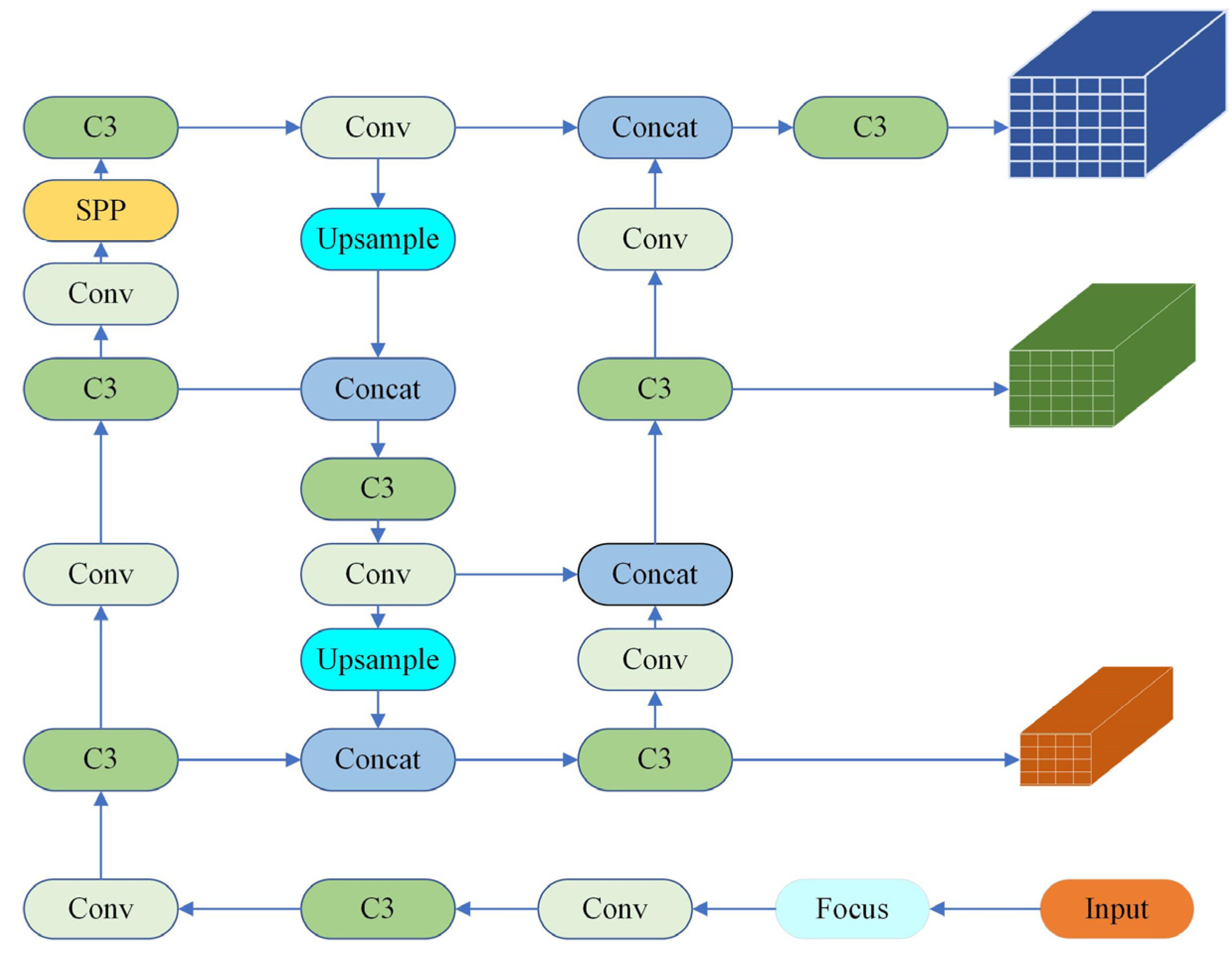
In order to reconstruct the scene using limited data, this study collected images of five typical landmark buildings at the campus of China University of Petroleum (Beijing), China. We collected data through a combination of mobile phone live scene collection and online image collection. The types of buildings we collected include two types of libraries, gymnasium, and two types of statues (some samples are shown in Figure 1). Considering the impact of different weather conditions, shooting angles, and lighting intensity on the detection effect in actual autonomous driving scenarios, we collected data from different seasons in the real scene collection, and the collection time was divided into morning, afternoon, and evening (corresponding to different lighting intensities). We also took photos of buildings at different angles to simulate real-world detection conditions. Due to the constantly changing visual fields during the driving process of autonomous vehicles, we changed the distance between the photographer and the building to obtain images in various visual fields, which fits actual applications. We collected a total of 1188 images, of which 784 were used as the training set, 236 were used as the testing set, and 168 were used as the validation set. Additionally, we use the LabelImg [36] tool for image annotation. LabelImg is an image annotation tool developed by Tzuhsal, which can be used to annotate YOLO format data. The labeling process for YOLO format data in labelImg is simple. Users can select rectangular boxes and adjust their position and size until the target object is included. Meanwhile, the files including labels are automatically generated and saved at the corresponding address. The LabelImg results of different buildings are shown in Figure 2. The sizes of the images we collected from the mobile phones are 3000 × 4000, 3264 × 2448, and 2448 × 3264. The YOLOv5 has the scaling function, which turns different sizes into the same size. In order to set all the sizes to the same, we use the scaling function in YOLOv5 to set all the sizes of images to 640 × 640, which is the default input size of YOLOv5.

However, the dataset we collected is limited and it cannot cover various environments. In order to solve these issues, we apply data augmentation to expand the dataset and enhance the robustness of images to various environments. Data augmentation is an important technique in deep learning, which can help improve the performance, generalization ability, and robustness of models while alleviating problems such as overfitting and class imbalance. The categories of data augmentation are various, and the most common ones are rotation, scaling, Cutout, and GridMask, etc. [31,37]. During the process of image acquisition, we observed irregular influences from the surrounding environment on the detection target. Factors like moving pedestrians and seasonal changes in trees contribute to these interferences, which can significantly affect detection accuracy. In real-world scenarios, occluded images often result in bad performance. To reduce the impact of occlusion on detection, we proposed a randomly distributed version of the GridMask data augmentation method, preprocessing our dataset, simulating actual occlusion situations, and enhancing the robustness of images to occlusion.

While GridMask [31] has proven effective in object detection tasks, its application in building detection tasks required a tailored approach. Due to the fact that building targets often occupy a relatively large area, using GridMask will occupy the entire building target, which may lead to the model learning from the patterns of GridMask and potentially affect its feature extraction ability. To address this, we refine the distribution of GridMask to randomly target areas within the image, which allows us to mimic the real-world conditions more accurately. Additionally, different from original GridMask, the improved GridMask fit in the occlusion situation in actual scenes because in the real scene, the occlusions tend to focus on a specific area of the image rather than the entire image. Following this thinking, we scale down GridMask in a random proportion. Lastly, as the location of occlusions in the actual identification process is random, we randomly distribute the GridMask in the image. By placing the GridMask in random areas, we aim to optimize our model’s performance specifically in detecting buildings with occlusions. This approach is designed to enhance both the accuracy and reliability of our model, ensuring its robustness in recognizing building under varied environmental conditions. Through experiments, it has been proven that our improved GridMask can effectively enhance the detection ability of the model.

The process of data augmentation, as illustrated in Figure 3, involves the introduction of randomly distributed GridMasks of different sizes into each image. These GridMasks are defined by parameters O, P, Q, and R, which respectively determine the position and size of the mask within the image. Within each GridMask, there are multiple unit domains, each comprising black and white blocks. The parameter a, alongside b, determines the size of the black blocks within these unit domains. Additionally, parameter r specifies the ratio of black blocks to the overall size of the mask.

2.2. The YOLOv5

YOLOv5 (You Only Look Once Version 5) is a commonly used single-stage object detection method with four modules in its structure: input, backbone, neck, and detection head. At the same time, YOLOv5 introduces four different scale models to adapt to different application scenarios: YOLOv5s, YOLOv5m, YOLOv5l, and YOLOv5x. The structure of YOLOv5 is shown in Figure 4 and the detailed introduction of every module is shown below.

(1) Input module: YOLOv5 adopts adaptive image scaling, which scales the input image to a size of 640 × 640. The K-Means algorithm is used to adaptively calculate the optimal anchor box based on the dataset. For feature maps with different output scales, each scale corresponds to three anchor boxes. The larger the feature map scale, the greater its spatial resolution. Additionally, YOLOv5 adopts data augmentations including Mosaic [38], Mixup [39], HSV augmentation, etc.

(2) Backbone module: the main function of the Backbone is to extract features through multi-layer convolution, which includes the Conv module (Figure 5a), C3 module (Figure 5b), and SPP module (Figure 5c). The Conv module (Figure 5a), where the BN channel pruning method can be implemented, consists of convolutional layers, batch normalization layers, and activation functions. The C3 module consists of three Conv modules and one bottleneck module (Figure 5b).

Figure 4. The structure of YOLOv5.

Figure 4. The structure of YOLOv5.

Figure 5. (a) The structure of Conv. (b) The structure of C3. (c) The structure of SPP. (d) The structure of FPN-PAN.

Figure 5. (a) The structure of Conv. (b) The structure of C3. (c) The structure of SPP. (d) The structure of FPN-PAN.

The SPP module is spatial pyramid pooling (Figure 5c). The Backbone part extracts image features through a series of convolutional and pooling layers. As the network depth increases, the feature map continuously shrinks and the corresponding receptive field continuously increases. The backbone network has built a multi-scale feature representation to assist YOLOv5 in extracting multi-scale features from images.

(3) Neck module: this module is responsible for feature fusion and processing, YOLOv5 integrates Feature Pyramid Networks (FPN) and Path Aggregation Networks (PAN) (Figure 5d). In the FPN structure, low resolution feature maps are magnified through up-sampling to recover lost information, and feature maps of different levels are concatenated. The PAN structure inputs multi-scale information fused by FPN and reduces the feature map size through down-sampling to increase the receptive field, performs deeper feature fusion with FPN’s feature maps, and outputs three different scale feature maps. The FCN-PAN structure enhances YOLOv5’s detection ability for targets of different sizes.

(4) Detection head module: this module contains three feature maps of different scales, corresponding to three prediction boxes of different scales. Each prediction box contains three pieces of information: confidence, category probability, and bounding box position. For the same object, there may be multiple target boxes. To avoid multiple detection of the same object, the detection head introduces Non-Maximum Suppression (NMS) to filter out duplicate target boxes and retain the optimal target box.

(5) The loss function of YOLOv5 includes three parts: localization loss, confidence loss, and classification loss. The confidence loss and classification loss are calculated through binary cross entropy, while the localization loss is calculated through Complete Intersection Over Union (CIOU). CIOU is a loss function based on Intersection Over Union (IOU), which incorporates the overlapping area, center point distance, and aspect ratio of predicted and actual boxes into the calculation, accelerating the convergence speed of the model. In the detection head component, which generates prediction boxes, YOLOv5 incorporates confidence, category probability, and bounding box position information. Post-processing steps include Non-Maximum Suppression (NMS) to filter duplicate detection and retain the optimal bounding boxes.

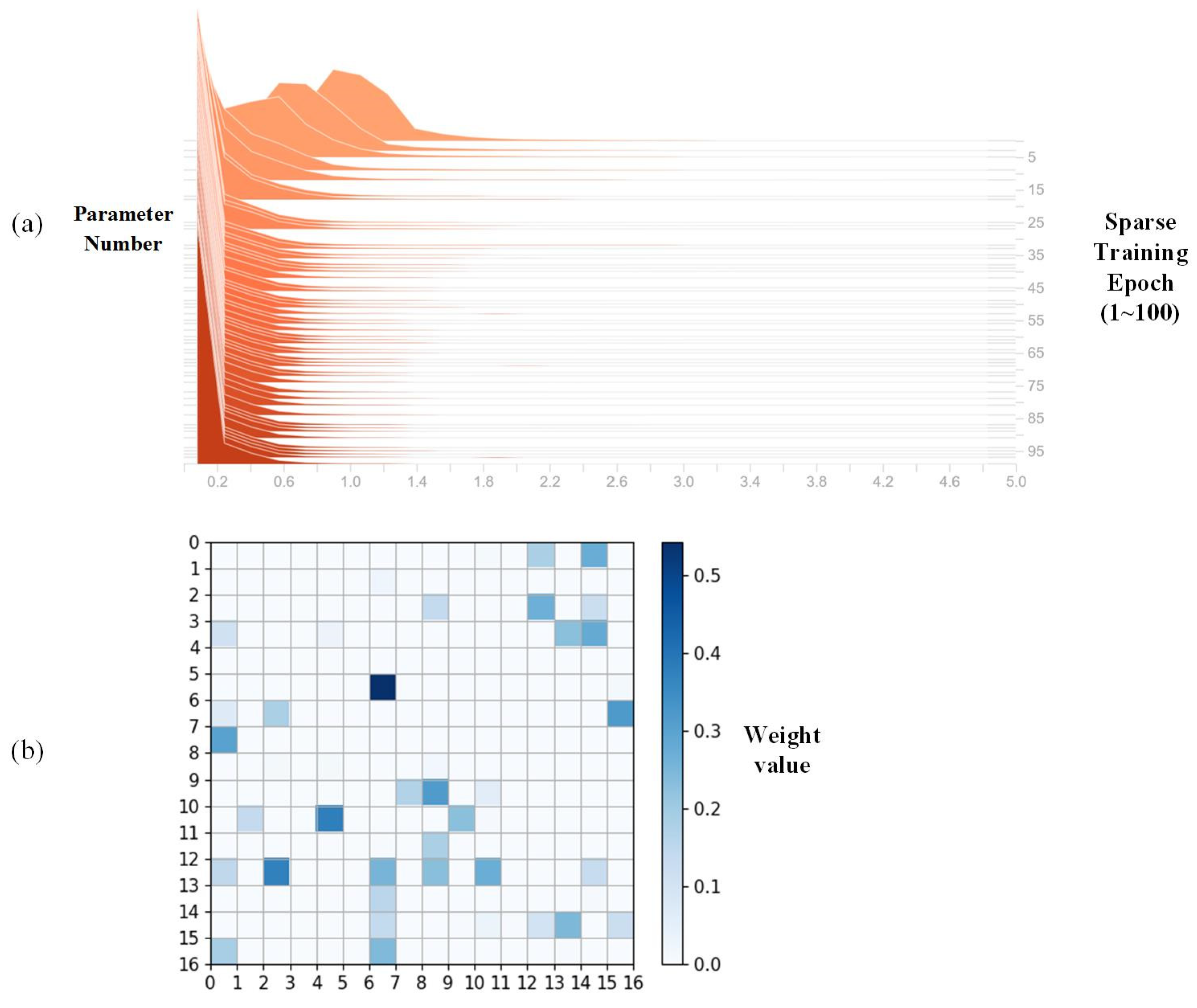
2.3. Sparse Training and Model Pruning

The Batch Normalization (BN) layer [32] is a data normalization layer proposed by Google in 2015, which is a very important structure in YOLOv5. The main purpose of the BN layer is to solve the internal covariate shift problem. The method is shown in Figure 6. The BN layer can effectively standardize the data distribution to a standard normal distribution with a mean of 0 and a variance of 1. Through this method, the data can be distributed in areas with high activation function gradients to alleviate the problem of vanishing gradients.

In BN layers, learnable parameters (γ and β) are introduced to enhance the efficiency of model training. When γ and β approach 0, the output of the BN layer tends towards 0 as well. This suggests that cutting off channels with small values of γ and β would have minimal impact on the network.

According to the theory outlined in [33,34], sparse training (Figure 7) is achieved by applying an L1 regularization penalty to the backpropagation gradient within the BN layer. This process makes γ and β approach 0, reducing the impact of pruning on model performance, enabling us to proceed with pruning while maintaining the network’s robustness and efficiency. Based on the results of sparse training, the pruning process involves eliminating channels with smaller values of γ and β while simultaneously pruning the convolutional kernels connected before and after the BN layers. Finally, it is necessary to fine-tune the model to compensate for the impact of pruning on its expressive ability after pruning.

We conducted this pruning method due to the fact that there are many BN layers in the structure of YOLOv5. The dense distribution of BN layers in YOLOv5 makes BN layer pruning effectively reduce the size of the model. Furthermore, most BN layers correspond one-to-one with the channels of the convolutional layers before and after (except for some BN layers with shortcut operation) in YOLOv5, which allows us to directly prune the corresponding channels of the convolutional layers before and after those BN layers.

2.4. Mish Activation Functions

Research has demonstrated that the selection of activation functions plays a crucial role in determining the performance of sparse networks [40]. In this study, we implement the Mish activation function due to its remarkable performance observed across a variety of datasets [41,42]. Proposed by Diganta Misra et al. in 2019, the Mish activation function presents itself as a novel addition to the repertoire of activation functions.

The Mish activation function (Figure 8), the formula of which is shown in Equations (1) and (2), operates by applying the softplus function to the input x, and the result is then passed through the hyperbolic tangent function (tanh). Finally, the result is multiplied by x to obtain the output. In pruned networks, a reduction in parameters may decrease the model’s expressive capacity, leading to accuracy loss. Mish’s non-linear mapping and smoothness enable networks to effectively utilize remaining parameters for feature extraction and learning. Moreover, Mish’s gradients are smoother near zero, mitigating gradient vanishing issues and enhancing training stability. Integrating Mish activation leverages its feature extraction and gradient smoothing capabilities to better compensate for accuracy loss due to pruning, enabling pruned models to maintain high efficiency while preserving accuracy.

$$Mish\left(x\right)=x\ast tanh\left(softplus\right(x\left)\right)$$

(1)

$$softplus\left(x\right)=log(1+e^x)$$

(2)

3. Experiments

3.1. Experiment Settings

We optimized model parameters using Adaptive Moment Estimation (Adam), with an initial learning rate of 0.001 and a final learning rate of 0.0001. We set the momentum to 0.937 and weight decay to 0.0005 to prevent overfitting. To improve model fitting, we conducted warm-up training, where the warm-up parameters warmup momentum and initial learning rate were set to 3 and 0.1, respectively. Additionally, we set the training epochs as 100 and the batch size as 16.

The hardware and software environments for developing the proposed model and conducting the experiments are shown in

Table 1. The hardware and software environments.

Item	Configuration
Operating system	CentOS Linux 8 (Core)
Processor	Intel(R) Xeon(R) Silver 4210 CPU @ 2.20 GHz
Video card	4 × NVIDIA Quadro RTX 4000
GPU internal storage	8 GB per GPU, total 32 GB for all GPUs (video RAM)
Programming language	Python 3.6.8
Deep learning framework	Pytorch1.8.1

.

3.2. Performance Metrics

For the comparison with the baseline model (i.e., YOLOv5s), precision (P), recall (R), [email protected], model size, the number of parameters, and GFLOPs are used to comprehensively evaluate the performance of the model. GFLOPs, standing for Giga Floating Point Of Operations, can be used to measure model complexity.

The formulas for calculating precision and recall are as follows.

$$P=\frac{TP}{TP+FP}$$

(3)

$$R=\frac{TP}{TP+FN}$$

(4)

TP (true positives) represents the number of accurately identified buildings. FP (false positives) represents the number of buildings mistakenly classified as positive. FN (false negatives) represents the number of buildings mistakenly classified as negative.

mAP is defined as follows:

$$AP={\int }_0^{1}P\left(R\right)dR$$

(5)

$$mAP=\frac{\sum _{i=1}^n{AP}_i}{n}$$

(6)

P represents precision, R represents recall, and AP is equal to the area under the precision-recall curve. mAP is the arithmetic mean of n categories of AP, while [email protected] represents mAP when Intersection over Union (IoU) = 0.50 as building targets in our dataset are mostly large objects.

3.3. Experimental Design

The overall process of building detection method is shown in Figure 9, which includes the following steps: (1) Data augmentation is performed on the dataset, and an improved GridMask method is used to introduce random noise for simulating actual occlusion situations. (2) Sparse training is performed on the improved model to make the parameters of the BN layer approach 0. (3) We crop the BN layer parameters according to the pruning rate. (4) We replace the activation function with Mish and compare its effectiveness with different activation functions.

4. Results and Analysis

4.1. Data Augmentation

Our improved GridMask randomly distributes masks in the image based on the original data augmentation method. After modification, the improved GridMask can better fit in the occlusions in real scenes. We used the improved GridMask to augment the entire training dataset and chose the suitable parameters to simulate the occlusions in our dataset. Given that the sizes of images in the training dataset were 3000 × 4000, 3264 × 2448, and 2448 × 3264, we set the parameters O and P to random numbers between 200 and 1800 and parameters Q and R to random numbers between 200 and 400. This was done to distribute the GridMask as closely to the target in the image as possible while also ensuring some overlap (the purpose of doing so is to simulate occlusion). Additionally, the parameter r was set to 0.5.

In order to verify the effectiveness of data augmentation, we assess the effectiveness of data augmentation by training YOLOv5s models with consistent parameters and comparing performance with and without data augmentation.

Table 2. Detection performance of YOLOv5s with and without data augmentation.

Model	Precision	Recall	[email protected]	Model Size	Parameters
Data augmentation	93.4%	86.6%	89.6%	14.070 MB	7,074,330
Without Data augmentation	94.9%	84.3%	89.5%	14.070 MB	7,074,330

presents the results which indicate that recall, and [email protected] values are improved notably when utilizing the improved GridMask in the building dataset. Notably, the model size and the number of parameters remain unchanged across both configurations. The results in Table 2 reveal that the model without data augmentation achieves a precision of 94.9%, a recall of 84.3.%, and a [email protected] of 89.5%. The model with data augmentation achieves a precision of 93.4%, a few points lower than the former model. That means that adding the improved Gridmask may lead the model to make a few mistakes when detecting some images. However, the recall of the model increases to 86.6%, which means the model with the improved GridMask can detect some images which cannot be detected by the former model.

To further verify the impact of the improved GridMask on occlusion, we chose all the images with occlusion from the test dataset (a total of 101 images) and tested the models with these images. The results are shown in

Table 3. Detection performance of YOLOv5s with and without data augmentation on images with occlusion.

Model	Precision	Recall	[email protected]	Model Size	Parameters
Data augmentation	93.1%	72.9%	80.0%	14.070 MB	7,074,330
Without Data augmentation	93.4%	68.3%	78.9%	14.070 MB	7,074,330

. Compared with the model without data augmentation, the model with improved GridMask significantly improves the recall metric by 4.6%. The precision of all the models is maintained at more than 93%. In the detection of occluded objects, the improved GridMask greatly improves the recall rate of the model, thus avoiding missed detections to some extent.

We take the gymnasium as an example because, as a category of object detection, gymnasiums often face serious occlusion problems, which adds difficulty to the object detection task. As shown in Figure 10a, two images exhibit a phenomenon of missed detection, while another image shows occurrence of false positives. However, gymnasiums in Figure 10b are successfully detected with data augmentation. As adding the improved GridMask can increase the data diversity, the model can learn more general features during training, rather than overfitting to detailed features. Due to the improved GridMask simulating occlusion, the model will not overly rely on specific features to detect objects when facing real-world disturbances. Therefore, the robustness of the model to occlusion is improved. Furthermore, the random distribution and size of the improved GridMask reduce the probability of the network learning from the feature of noise, thus maintaining the recall of the model.

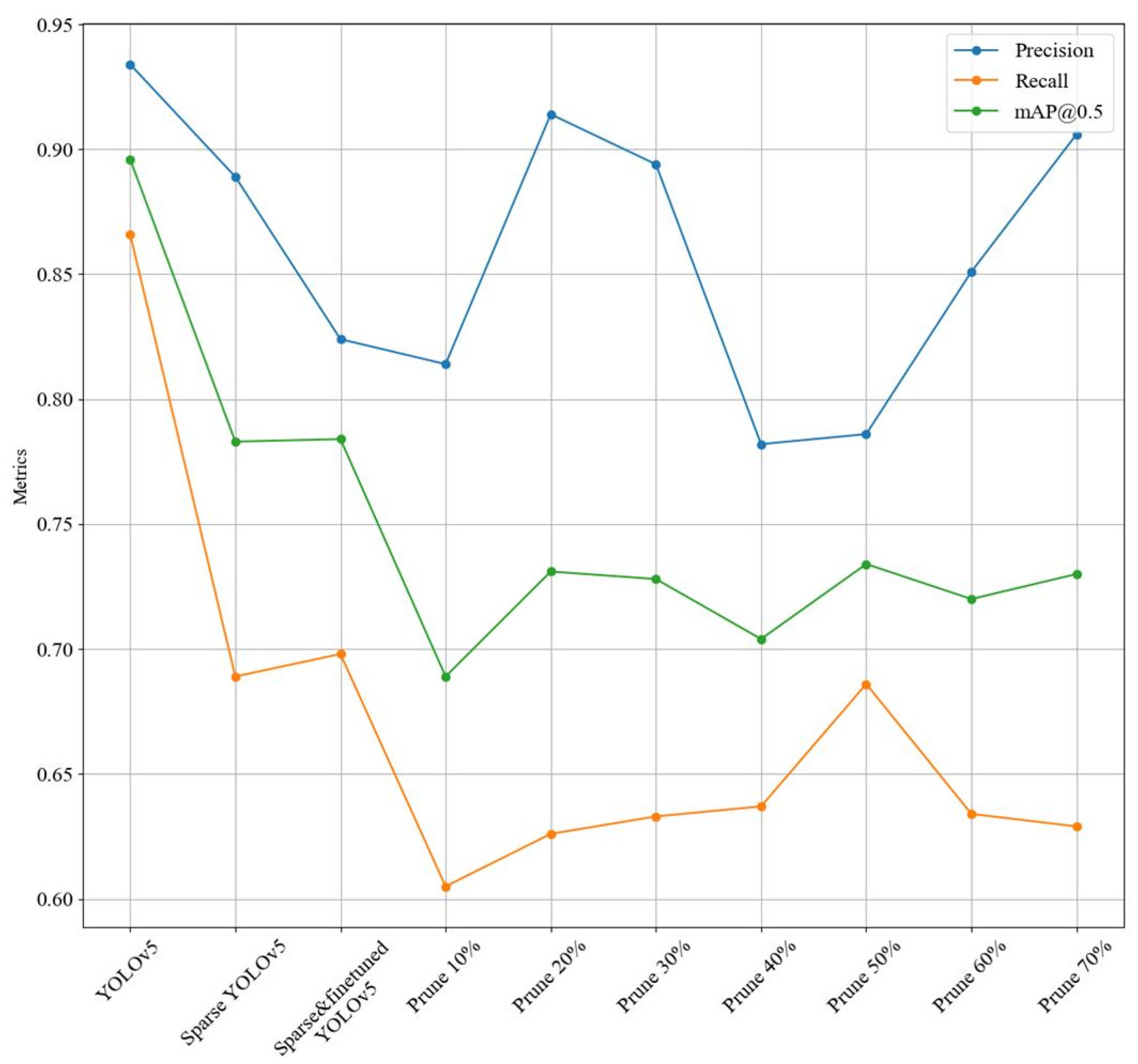
4.2. BN Layer Pruning

In embedded devices with limited memory resources, the number of model parameters needs to be reduced for the deployment of model. To reduce the number of parameters, we applied BN layers pruning method on our model. The process includes sparse training, pruning, and fine-tuning. The purpose of sparse training is to make the structure of model sparse to minimize the impact of pruning on model accuracy. Through the sparse training process, we set the value of λ to be 0.0001 to ensure that our model can learn sparse representations effectively. Then, we sort the values of γ and β, pruning the channels with low values according to the pruning rate, and delete channels corresponding to smaller parameters. After the sparse training and pruning, the fine-tuning is implemented on the model to update the parameters of the pruned model. After pruning, the model does not require too many training epochs to fit. The epoch of fine-tuning training was set to 10.

During sparse training, the weight distribution of BN layers becomes sparse. Figure 11a illustrates the weights’ change during sparse training. The vertical axis represents the number of parameters, and the higher the height of the curve corresponding to each parameter value on the horizontal axis, the larger the number of parameters distributed at this parameter value. As the number of training epoch increases, the distribution of weights continuously concentrates towards 0, which means the sparse training can make the parameters sparse. When the L1 regularization is added to the loss function of γ, the direction of parameter updating is changed, and the feature selection effect of L1 regularization leads to some γ parameters approaching 0, thus resulting in parameter sparsity. Figure 11b shows the weights in one BN layer of the model (similar to other BN layers as the value of λ remain the same in all BN layers). In the heatmap, one parameter corresponds to one grid, and it is evident that the parameters are sparse in this BN layer. Those parameters that do not approach zero are more important in neural networks and should not be pruned.

In order to evaluate the impact of the three stages (sparse training, pruning, and fine-tuning) in the pruning process on the detection performance of YOLOv5s, we compared four different models including the original YOLOv5 (YOLOv5), sparse-trained models (Sparse YOLOv5), the model which is sparse and fine-tuned (Sparse and fine-tuned YOLOv5), and the pruned model with different pruning rates (Pruned YOLOv5 (pruning rate)). The pruning rates are varied from 10% to 90%, with an interval of 10%. The experimental results are shown in Figure 12 and

Table 4. Detection performance of different models in model size, parameter, and GFLOPs.

Model	Model Size (MB)	Parameters	GFLOPs
YOLOv5	14.070	7,074,330	16.5
Sparse YOLOv5	27.931	7,074,330	16.5
Sparse and fine-tuned YOLOv5	14.120	7,074,330	16.5
Prune YOLOv5 (0.1)	12.425	6,209,872	14.8
Prune YOLOv5 (0.2)	10.731	5,344,219	13.5
Prune YOLOv5 (0.3)	9.195	4,559,893	12.3
Prune YOLOv5 (0.4)	7.873	3,884,554	11.1
Prune YOLOv5 (0.5)	6.685	3,277,868	10.2
Prune YOLOv5 (0.6)	5.606	2,727,398	9.2
Prune YOLOv5 (0.7)	4.475	2,150,031	7.6
Prune YOLOv5 (0.8)	-	-	-
Prune YOLOv5 (0.9)	-	-	-

.

As shown in Table 4, when the pruning rates increase, the model size and number of parameters decrease, indicating that the pruning method can effectively reduce the size of the model. The pruning process can delete unimportant channel in BN layers, reducing the number of parameters. In this way, the model can be integrated to devices with limited memory. Furthermore, the GFLOPs also declines when increasing the pruning rate. When some channels of the model are deleted, the computational complexity of the model decreases accordingly, resulting in a decrease in GFLOPs. When the hardware conditions are the same, decreasing the computational complexity of the model can enhance the calculation speed of the model. Therefore, model pruning can improve the computational speed of the model, which is significant for autonomous driving.

In Figure 12, it is evident that the relationship between pruning rate and model performance metrics such as accuracy and recall is not straightforward. While we might expect these performance metrics to decrease as the pruning rate increases, the experimental results reveal that the model achieves its lowest accuracy around the 40–50% pruning rate. This suggests that there is a non-linear relationship between pruning rate and model performance. Moreover, the comparison between the YOLOv5 and Pruned YOLOv5 highlights a significant reduction in [email protected] and recall for Pruned YOLOv5. This indicates that although pruning effectively reduces the number of parameters, it can also lead to a decrease in the model’s detection ability. Therefore, the pruning process has a negative impact on the detection performance of the model and there is a trade-off between model size reduction and maintaining high detection performance. Additionally, the comparison between Sparse YOLOv5 and YOLOv5 further emphasizes the impact of sparse training on model detection ability. The lower [email protected] of sparse-trained models, even after fine-tuning, suggests that sparse training alone can decrease the model’s detection ability. Furthermore, the limited effect of fine-tuning on recovering model accuracy indicates that additional strategies may be required to mitigate the negative effects of sparse training on model performance.

In summary, while pruning can effectively reduce the number of parameters, it can also impair the detection ability of the model. Sparse training alone may also decrease model performance, and the effectiveness of fine-tuning in recovering model accuracy may be limited. Therefore, additional techniques may be necessary to find a balance between model size reduction and maintaining high detection performance.

4.3. Comparison of Different Activation Functions

As the activation function has a significant impact on sparse training, we replaced the activation function with Mish/HardSwish/Leaky ReLU/RReLU for sparse training, and set the pruning rates to 30%, 50%, and 70%, respectively. We conducted ablation experiments to compare the impact of different activation functions on the detection performance of the model under sparse training. The experimental results are shown in Figure 13.

When the pruning rate is set at 30%, Mish consistently outperforms other activation functions in terms of [email protected] and precision (with 82.9% and 94.4%, respectively), while Leaky ReLU exhibits the lowest recall (68.2%) and [email protected] (77.7%). Although the [email protected] values of HardSwish and RReLU are slightly lower than that of Mish, the overall results highlight Mish’s robustness and effectiveness in preserving information, particularly at lower pruning rates. Moreover, when the pruning rate is 50%, it is clearly that the three indexes of Mish are higher than that of other activation function (precision is 93.1%, recall is 73.4%, and [email protected] is 81.8%). However, at a pruning rate of 70%, Leaky ReLU shows higher recall compared to other activation functions with 76.3%, yet Mish still performs best in [email protected] and precision with 82.3% and 91.8%, respectively. This underscores Mish’s capacity to compensate for accuracy loss induced by pruning. The inherent characteristics of Mish, such as non-linear mapping and smoothness, likely contribute to this capability, enabling the model to better maintain object detection and classification accuracy even under high pruning rates. On the other hand, despite Leaky ReLU demonstrating the highest recall at a 70% pruning rate, its overall performance metrics fall short compared to Mish and other activation functions. This could be due to Leaky ReLU’s limited ability to maintain precision and overall classification accuracy.

Regarding the effects of increasing pruning rates, comparisons can also be conducted by inspecting Figure 13. When using the Mish activation function, the precision of the corresponding model decreases but remains higher than 90%, while the [email protected] and recall are the lowest at 50% pruning rates. As for HardSwish, it is evident that a higher pruning rate leads to higher precision and lower recall, with the [email protected] staying highest at the 50% pruning rate. This result contrasts with that of Mish. Leaky ReLU and RReLU are improved activation functions of ReLU, with RReLU performing much better than Leaky ReLU in terms of [email protected]. This difference may be attributed to the introduction of random parameters in RReLU.

The effect of different activation functions on the model performance can be attributed to the mechanism of gradient backpropagation and sparse training. As for a Conv module (Figure 5a), the gradient of backpropagation will be transmitted from the activation function gradient to the BN layer for updating the BN layer parameters. The whole process is shown in Figure 14. The gradient of the loss function with respect to BN layer parameters consists of four parts: the gradient of the BN layer output with respect to the BN layer parameter γ and β, gradient of activation function, the gradient of loss function with respect to activation function’s output, and the gradient changes brought about by L1 regularization. The gradient of the BN layer output with respect to the BN layer parameter and that of the loss function with respect to activation function’s output depend on the input and output of the network. Furthermore, the gradient changes generated from L1 regularization are constant. Therefore, the gradient of the loss function with respect to BN layer parameters can be different with different activation functions, and different activation functions can affect the impact of L1 regularization on gradient updating, thereby affecting the effectiveness of sparse training.

5. Conclusions

In this study, we proposed a lightweight building detection model based on YOLOv5s. We modified GridMask to a random size and placed it in random places in images, as the original GridMask may entirely cover the building, which may cause excessive loss of features in the original image. In this way, we can get a balance between stability and adaptability of model, increasing the robustness of model to occlusion. Then, we pruned the model with the BN-Layers pruning method, which successfully reduced the volume of model by 70%. Finally, we compared different activation functions in our pruning model and proved that the Mish can help reduce the impact of pruning on the model. The results showed that the side effects of pruning can be relieved through selection of appropriate activation functions. It also should be noted that the improved YOLOv5s model for building detection can be used not only on campus buildings but also in various area such as tourist attractions, city navigation, etc. By recognizing buildings and other urban features, autonomous vehicles can enhance their localization techniques, especially in GPS-denied environments.

References

1. Wu, J.; Huang, Z.; Lv, C. Uncertainty-Aware Model-Based Reinforcement Learning: Methodology and Application in Autonomous Driving. IEEE Trans. Intell. Veh. 2023, 8, 194–203. [Google Scholar] [CrossRef]
2. Xiao, Y.; Zhang, X.; Xu, X.; Liu, X.; Liu, J. Deep Neural Networks with Koopman Operators for Modeling and Control of Autonomous Vehicles. IEEE Trans. Intell. Veh. 2023, 8, 135–146. [Google Scholar] [CrossRef]
3. Teng, S.; Chen, L.; Ai, Y.; Zhou, Y.; Xuanyuan, Z.; Hu, X. Hierarchical Interpretable Imitation Learning for End-to-End Autonomous Driving. IEEE Trans. Intell. Veh. 2023, 8, 673–683. [Google Scholar] [CrossRef]
4. Li, J.; Allinson, N. Building recognition using local oriented features. IEEE Trans. Ind. Inform. 2013, 9, 1697–1704. [Google Scholar] [CrossRef]
5. Hascoët, N.; Zaharia, T. Building recognition with adaptive interest point selection. In Proceedings of the 2017 IEEE International Conference on Consumer Electronics (ICCE), Las Vegas, NV, USA, 8–10 January 2017; pp. 29–32. [Google Scholar] [CrossRef]
6. Lecun, Y.; Bottou, L.; Bengio, Y.; Haffner, P. Gradient-based learning applied to document recognition. Proc. IEEE 1998, 86, 2278–2324. [Google Scholar] [CrossRef]
7. Krizhevsky, A.; Sutskever, I.; Hinton, G.E. ImageNet classification with deep convolutional Neural Networks. Commun. ACM 2017, 60, 84–90. [Google Scholar] [CrossRef]
8. Simonyan, K.; Zisserman, A. Very Deep Convolutional Networks for Large-Scale Image Recognition. In Proceedings of the 3rd International Conference on Learning Representations, San Diego, CA, USA, 7–9 May 2015; pp. 1–14. [Google Scholar]
9. Szegedy, C.; Liu, W.; Jia, Y.; Sermanet, P.; Reed, S.; Anguelov, D.; Erhan, D.; Vanhoucke, V.; Rabinovich, A. Going deeper with convolutions. In Proceedings of the 38th IEEE Conference on Computer Vision and Pattern Recognition, Boston, MA, USA, 7–12 June 2015; pp. 1–9. [Google Scholar]
10. Girshick, R.; Donahue, J.; Darrell, T.; Malik, J. Rich feature hierarchies for accurate object detection and semantic segmentation. In Proceedings of the 37th IEEE Conference on Computer Vision and Pattern Recognition, Columbus, OH, USA, 23–28 June 2014; pp. 580–587. [Google Scholar]
11. Girshick, R. Fast R-CNN. In Proceedings of the 15th IEEE International Conference on Computer Vision, Santiago, Chile, 7–13 December 2015; pp. 1440–1448. [Google Scholar]
12. Ren, S.; He, K.; Girshick, R.; Sun, J. Faster R-CNN: Towards Real-Time Object Detection with Region Proposal Networks. In Proceedings of the 28th International Conference on Neural Information Processing Systems, Montreal, QC, Canada, 8–13 December 2015; pp. 91–99. [Google Scholar]
13. Redmon, J.; Divvala, S.; Girshick, R.; Farhadi, A. You only look once: Unified, real-time object detection. In Proceedings of the 39th IEEE Conference on Computer Vision and Pattern Recognition, Las Vegas, NV, USA, 27–30 June 2016; pp. 779–788. [Google Scholar]
14. Liu, W.; Anguelov, D.; Erhan, D.; Szegedy, C.; Reed, S.; Fu, C.Y.; Berg, A.C. SSD: Single shot multibox detector. In Proceedings of the 14th European Conference on Computer Vision, Amsterdam, The Netherlands, 11–14 October 2016; pp. 21–37. [Google Scholar]
15. Guo, G.; Zhang, Z. Road damage detection algorithm for improved YOLOv. Sci. Rep. 2022, 12, 15523. [Google Scholar] [CrossRef]
16. Howard, A.; Sandler, M.; Chu, G.; Chen, L.; Chen, B.; Tan, M. Searching for MobileNetV3. In Proceedings of the 2019 IEEE/CVF International Conference on Computer Vision (ICCV), Seoul, Republic of Korea, 27 October–2 November 2019; pp. 1314–1324. [Google Scholar]
17. Xu, H.; Li, B.; Zhong, F. Light-YOLOv5: A Lightweight Algorithm for Improved YOLOv5 in Complex Fire Scenarios. Appl. Sci. 2022, 12, 12312. [Google Scholar] [CrossRef]
18. Zhu, X.; Lyu, S.; Wang, X.; Zhao, Q. TPH-YOLOv5: Improved YOLOv5 based on transformer prediction head for object detection on drone-captured scenarios. In Proceedings of the IEEE/CVF International Conference on Computer Vision, Montreal, BC, Canada, 11–17 October 2021; pp. 2778–2788. [Google Scholar]
19. Vaswani, A.; Shazeer, N.; Parmar, N.; Uszkoreit, J.; Jones, L.; Gomez, A.N.; Kaiser, Ł.; Polosukhin, I. Attention is all you need. Adv. Neural Inf. Process. Syst. 2017, 30, 5998–6008. [Google Scholar]
20. Bezak, P. Building recognition system based on deep learning. In Proceedings of the 2016 Third International Conference on Artificial Intelligence and Pattern Recognition (AIPR), Lodz, Poland, 19–21 September 2016; pp. 1–5. [Google Scholar]
21. Zheng, L.; Ai, P.; Wu, Y. Building Recognition of UAV Remote Sensing Images by Deep Learning. In Proceedings of the IGARSS 2020—2020 IEEE International Geoscience and Remote Sensing Symposium, Waikoloa, HI, USA, 26 September–2 October 2020; pp. 1185–1188. [Google Scholar]
22. Chen, J.; Li, T.; Zhang, Y.; You, T.; Lu, Y.; Tiwari, P.; Kumar, N. Global-and-Local Attention-Based Reinforcement Learning for Cooperative Behaviour Control of Multiple UAVs. IEEE Trans. Veh. Technol. 2024, 73, 4194–4206. [Google Scholar] [CrossRef]
23. Ju, C.; Son, H. Multiple UAV Systems for Agricultural Applications: Control, Implementation, and Evaluation. Electronics 2018, 7, 162. [Google Scholar] [CrossRef]
24. Yang, T.; Li, P.; Zhang, H.; Li, J.; Li, Z. Monocular Vision SLAM-Based UAV Autonomous Landing in Emergencies and Unknown Environments. Electronics 2018, 7, 73. [Google Scholar] [CrossRef]
25. Li, X.; Fu, L.; Fan, Y.; Dong, C. Building Recognition Based on Improved Faster R-CNN in High Point Monitoring Image. In Proceedings of the 33rd Chinese Control and Decision Conference (CCDC), Kunming, China, 22–24 May 2021; pp. 1803–1807. [Google Scholar]
26. Han, K.; Wang, Y.; Tian, Q.; Guo, J.; Xu, C.; Xu, C. GhostNet: More Features from Cheap Operations. In Proceedings of the 2020 IEEE/CVF Conference on Computer Vision and Pattern Recognition (CVPR), Seattle, WA, USA, 13–19 June 2020; pp. 1577–1586. [Google Scholar]
27. Tang, Y.; Han, K.; Guo, J.; Xu, C.; Xu, C.; Wang, Y. GhostNetV2: Enhance Cheap Operation with Long-Range Attention. arXiv 2022, arXiv:2211.12905. [Google Scholar]
28. Guo, Y.; Chen, S.; Zhan, R.; Wang, W.; Zhang, J. LMSD-YOLO: A lightweight YOLO algorithm for multi-scale SAR ship detection. Remote Sens. 2022, 14, 4801. [Google Scholar] [CrossRef]
29. Dang, C.; Wang, Z.; He, Y.; Wang, L.; Cai, Y.; Shi, H.; Jiang, J. The Accelerated Inference of a Novel Optimized YOLOv5-LITE on Low-Power Devices for Railway Track Damage Detection. IEEE Access 2023, 11, 134846–134865. [Google Scholar] [CrossRef]
30. Xu, K.; Zhang, H.; Li, Y.; Zhang, Y.; Lai, R.; Liu, Y. An Ultra-Low Power TinyML System for Real-Time Visual Processing at Edge. IEEE Trans. Circuits Syst. II Express Briefs 2023, 70, 2640–2644. [Google Scholar] [CrossRef]
31. Chen, P.; Liu, S.; Zhao, H.; Jia, J. GridMask data augmentation. arXiv 2020, arXiv:2001.04086. [Google Scholar]
32. Ioffe, S.; Szegedy, C. Batch normalization: Accelerating deep network training by reducing internal covariate shift. In Proceedings of the International Conference on Machine Learning, Lille, France, 6–11 July 2015; pp. 448–456. [Google Scholar]
33. Li, H.; Kadav, A.; Durdanovic, I.; Samet, H.; Graf, H.P. Pruning filters for efficient convnets. arXiv 2016, arXiv:1608.08710. [Google Scholar]
34. Liu, Z.; Li, J.; Shen, Z.; Huang, G.; Yan, S.; Zhang, C. Learning efficient convolutional networks through network slimming. In Proceedings of the IEEE International Conference on Computer Vision, Venice, Italy, 22–29 October 2017; pp. 2736–2744. [Google Scholar]
35. Misra, D. Mish: A self regularized non-monotonic activation function. arXiv 2019, arXiv:1908.08681. [Google Scholar]
36. Tzutalin. LabelImg. Git Code (2015). Available online: https://github.com/tzutalin/labelImg (accessed on 31 March 2022).
37. De Vries, T.; Taylor, G.W. Improved regularization of convolutional neural networks with cutout. arXiv 2017, arXiv:1708.04552. [Google Scholar]
38. Bochkovskiy, A.; Wang, C.Y.; Liao, H.Y.M. YOLOv4: Optimal Speed and Accuracy of Object Detection. arXiv 2020, arXiv:2004.10934. [Google Scholar]
39. Zhang, H.Y.; Cissé, M.; Dauphin, Y.N.; Lopez-Paz, D. Mixup: Beyond empirical risk minimization. In Proceedings of the 6th International Conference on Learning Representations, Vancouver, BC, Canada, 30 April–3 May 2018; pp. 1–13. [Google Scholar]
40. Dubowski, A. Activation Function Impact on Sparse Neural Networks. Bachelor’s Thesis, University of Twente, Enschede, The Netherlands, 2020. [Google Scholar]
41. Dubey, S.R.; Singh, S.K.; Chaudhuri, B.B. Activation functions in deep learning: A comprehensive survey and benchmark. Neurocomputing 2022, 503, 92–108. [Google Scholar] [CrossRef]
42. Jagtap, A.D.; Karniadakis, G.E. How important are activation functions in regression and classification? A survey, performance comparison, and future directions. J. Mach. Learn. Model. Comput. 2023, 4, 21–75. [Google Scholar] [CrossRef]
Figure 1. Some examples of the dataset: (b,e) are the first type of library, (d,g) are the first type of statue, (c,i) are the second type of library, (a) is the second type of statue, and (f,h) is the gymnasium.
Electronics 13 02197 g001
Figure 2. Some examples of labeled results of different buildings (coordinate information) by LabelImg.
Electronics 13 02197 g002
Figure 3. The process of data augmentation.
Electronics 13 02197 g003
Figure 6. The method of BN layer.
Electronics 13 02197 g006
Figure 7. The process of sparse training and pruning.
Electronics 13 02197 g007
Figure 8. Mish activation function.
Electronics 13 02197 g008
Figure 9. The process of building detection method.
Electronics 13 02197 g009
Figure 10. Gymnasium detection with and without data augmentation.
Electronics 13 02197 g010
Figure 11. (a) Weights change in BN layers during sparse training process. (b) Weights in one BN layer of the model after sparse training (model.23.m.0.cv1.bn.weight).
Electronics 13 02197 g011
Figure 12. Detection performance of different models in precision, recall, and [email protected].
Electronics 13 02197 g012
Figure 13. Comparison between different activation functions with different pruning rates in YOLOv5.
Electronics 13 02197 g013
Figure 14. The process of the gradient of backpropagation in Conv module.
Electronics 13 02197 g014