Revealing GLCM Metric Variations across a Plant Disease Dataset: A Comprehensive Examination and Future Prospects for Enhanced Deep Learning Applications

Abstract

This study highlights the intricate relationship between Gray-Level Co-occurrence Matrix (GLCM) metrics and machine learning model performance in the context of plant disease identification. It emphasizes the importance of rigorous dataset evaluation and selection protocols to ensure reliable and generalizable classification outcomes. Through a comprehensive examination of publicly available plant disease datasets, focusing on their performance as measured by GLCM metrics, this research identified dataset_2 (D2), a database of leaf images, as the top performer across all GLCM analyses. These datasets were then utilized to train the DarkNet19 deep learning model, with D2 exhibiting superior performance in both GLCM analysis and DarkNet19 training (achieving about 91% testing accuracy) according to performance metrics such as accuracy, precision, recall, and F1-score. The datasets other than dataset_1 and 2 exhibited significantly low classification performance, particularly in supporting GLCM analysis. The findings underscore the need for transparency and rigor in dataset selection, particularly given the abundance of similar datasets in the literature and the growing trend of utilizing deep learning methods in future scientific research.

1. Introduction

In recent times, the world has faced an increase in population that in turn calls for a red alarm on food security. According to the Food and Agricultural Organization of the United Nations (FOA), a 70% increase in global food production is needed by the year 2050 to keep up with the abounding population [1]. This poses a serious demand on agriculture to rapidly and sustainably keep up with the foreseen population. However, since plants are the primary source of food, we face serious challenges in growing them. Abnormalities in their growth, mainly caused by diseases, pests, and environmental factors, have not yet been eliminated.

Plant diseases can cause anything from modest symptoms to severe damage to large fields of crops, incurring significant expenditures and having a significant negative influence on the agricultural economy. Plant pests and diseases account for about 40% loss of global food crops and trade loss of over USD 220 billion every year [2]. These diseases, promoted by invisible pathogens, pose the most serious effect on plants’ health [3], thus causing a significant threat to food security and affecting the environment. In addition, it has been noticed lately that recent climate change has promoted plant health problems via the early appearance of pests and their dissemination to areas where they have never been noticed [4].

Since ancient times, human beings have been struggling to counter these plant health problems. They largely rely on visible changes to plant parts, such as the leaves and stems, due to the absence of enough technology to detect their appearance early, hence causing a huge loss that may lead to famine in some regions [5]. This method is time- and resource-consuming, full of uncertainty, and labor-intensive. Moreover, traditional methods mainly focused on particular locations, thus limiting their efficiency across geographies. In contrast, plant diseases can spread across geographies unknowingly, bringing about a need for a more generalized system of detection [6].

With the advancements in technology, the world of today has been developing several techniques to tackle these problems. Artificial intelligence brought tremendous novelty in the name of machine learning and deep learning, which are currently relied on in these regards. Machine learning techniques have been widely used in the research community for the last two decades, during which time their applications were addressed and studies for agriculture and plant diseases were widely evaluated [7]. Conventional machine learning methods, however, still require time-consuming feature extraction for training models [8,9]. Moreover, they have limited success under some circumstances, such as the inability to process natural data in their raw form [5,10]. As a result, deep learning algorithms that automatically extract features as part of their natural operation have been incorporated into research for about a decade [11,12,13]. According to [14], deep learning has emerged as a preferred method for plant disease detection and management due to its increased computing power, storage capabilities, and accessibility of big datasets.

Deep learning simply learns from datasets of past disease images to detect and identify the plants’ health problem(s) using some sets of complex algorithms. As a data-hungry technology, research is being carried out on the use of deep learning battles with the preparation of datasets for individual applications. This has resulted in scientific research communities providing datasets for public use, simplifying the path for model development, learning, and knowledge sharing. The PlantVillage Dataset, developed by Hughes et al. [15], is considered one of the most significant datasets and has fueled the application of deep learning in plant disease detection and management [16,17,18,19]. The maize plant disease dataset [20], Digipathos dataset [21], multiple plant disease datasets [22], the PlantDoc dataset [23], the cassava disease image dataset [24], and the RoCoLe coffee disease dataset [25] are typical examples of the available plant disease datasets. The preparation of datasets for machine-learning- or deep-learning-based applications can also be performed by capturing images of live plants over a period using remote sensing and hyperspectral imagery [26]. Thermal imagery has also recorded success in capturing such images [27].

However, after a critical review and pre-tests undergone for the purpose of this study, most of the open datasets for plant disease detection were observed to possess a number of technical problems worthy of noting for deep learning applications. For example, many of the publicly available datasets such as the PlantVillage dataset were developed in controlled laboratory contexts. This controlled environment provides for exact control over variables, ensuring standardized data-gathering conditions. Though the authors of [28] trained a deep convolutional neural network (DCNN) with the PlantVillage dataset using AlexNet and GoogleNet architectures and obtained a performance efficiency of 99.35%, the controlled setting may not entirely mirror real-world situations encountered by farmers. In lab settings, field factors such as fluctuating light intensities, various backgrounds, and unpredictable weather are not faithfully duplicated. As a result, models trained on such datasets may perform poorly when applied to real-world agricultural contexts [29]. While these datasets give useful insights and initial model training, there is an urgent need to supplement them with field-based data to improve the resilience and practical application of deep learning models for plant disease detection. The works of [30,31] tangibly proved the high efficiency of models trained with field-based datasets.

Moreover, the size and resolution of the images offered in open plant disease datasets frequently vary. Some datasets contain very high-resolution images, like the RoCoLe coffee disease dataset [25] and the Paddy Doctor dataset [32], while others may contain images of inferior quality. For model training, images with high resolution can be computationally intensive and may necessitate large processing resources. Low-resolution images, on the other hand, may lack the fine-grained features necessary for effective disease detection. It is thus critical to strike a balance between image resolution and processing efficiency. To standardize image sizes in this case, preprocessing procedures are necessary to ensure that models can handle the data successfully while preserving the key visual information [31,33].

Plant diseases are extremely diverse, with hundreds of distinct pathogens affecting thousands of different plant species [6]. Each disease has unique symptoms, making it difficult to create a single universal dataset that includes all possible disease variations. Diseases can present differently even among the same plant species depending on factors such as pathogen strain, climatic circumstances, and host genetics [34]. Because of these complications, dedicated datasets for individual diseases or groups of linked disorders are necessary.

Plant disease databases have been created in certain cases by directly collecting photos from search engine results, most notably from platforms such as Google [35]. While this strategy may appear to be convenient, it creates numerous serious obstacles to the datasets’ integrity and trustworthiness. These photos lack consistent quality and metadata and thus may be in violation of copyright laws. Because of search engine biases, their diversity and representativeness are jeopardized. Stringent data-gathering techniques from trustworthy and authorized sources are thus required to ensure valid and reliable plant disease datasets. This not only maintains ethical norms but also improves the datasets’ quality and usability for relevant scientific research and deep learning applications in plant pathology.

Researchers are, nevertheless, expected to be mindful of the constraints imposed by specialized datasets. While they are useful for some disease categories, they may not be appropriate for broader applications without further data augmentation or transfer learning approaches, especially for open-field generated datasets for mobile application development.

Using texture analysis methods, including Gray-Level Co-occurrence Matrix (GLCM) metrics, which identify complex texture qualities in images, is one way to tackle these problems [36,37]. These metrics offer a quantitative depiction of texture features and offer insightful information about the spatial correlations between pixel intensities [38,39]. Nevertheless, little is known about how machine learning model performance is impacted by differences in GLCM metrics between datasets.

Progress in the field of plant disease identification depends on the scientific community’s ability to comprehend how differences in GLCM variables affect machine learning model performance. Along with providing insight into which datasets are appropriate for training models, it also helps to build reliable, broadly applicable models that are able to diagnose plant diseases in a variety of agricultural contexts. Consequently, it is imperative to conduct a thorough analysis of the differences in GLCM metrics among diverse plant disease datasets and evaluate their consequences for improved deep-learning applications in plant disease identification. This research is therefore an attempt to define novel criteria, using some publicly available plant disease datasets in the eyes of deep learning applications, through the exploration of technical and textual features of plant disease datasets for the enhancement of machine learning and deep learning applications, as the case may be.

2. Methodology

2.1. Data Collection

A set of five distinct plant disease datasets that are publicly available were acquired online:

• “plant_village dataset”;
• “a_database_of_leaf_images”;
• “RoCoLe dataset”;
• “FGVCx_cassava dataset” and
• “paddy_doctor dataset”.

Each of these datasets comprises a set of diverse plant species, diseases, and image resolutions.

2.2. Image Preprocessing and GLCM Metrics

Standardized image sizes and formats across datasets were captured and summarized using the Image Text analysis feature in the Python programming language interface.

The Gray Level Co-occurrence Matrix (GLCM) was used in the further processing of these datasets to obtain the relevant GLCM metrics. These are texture features derived from images that describe spatial relationships between pixel intensities. A total of ten (10) GLCM metrics, including energy, contrast, correlation, homogeneity, total variance, difference variance, maximum probability, joint entropy, difference entropy, and angular second moment, were extracted using predefined parameters and utilized for further analysis.

2.3. Statistical Analysis

Descriptive statistics was employed to compute and derive insights into the datasets. These include computed mean, variance, and sums of GLCM metrics for each dataset. Checks for the normality and homogeneity of data were conducted in an attempt to assess normal distribution assumptions using Shapiro–Wilk and Kolmogorov–Smirnov tests using GraphPad Prism 10.1.2 (324). The Kruskal–Wallis test was applied for non-normally distributed data for variability assessment. Several charts as figures were generated to display correlations and distributions in GLCM metrics. Relationships between these metrics within the datasets were also presented and are discussed in the results sections.

2.4. Deep Learning Model Training and Evaluation

From each dataset, 77 images were randomly collected (minimum number of classes available from the properties of the overall dataset used herein) to ensure uniformity as well as avoid bias in the representation of datasets. A total of 6160 images were summed from the different classes across the datasets and used as training data.

According to a conventional procedure, a deep learning model was trained independently with regard to each dataset. The following procedures were part of the training process:

(i)

Preprocessing of the Data: To improve model performance and better feature representation and guarantee uniformity before processing, the images were resized to a uniform resolution (227 × 227) and pixel values.

(ii)

Model Selection: The DarkNet19 architecture was chosen as the foundational model for training since it has a track record of success in image classification challenges. DarkNet19 is a deep convolutional neural network (CNN) model.

(iii)

Hyperparameter Tuning: To maximize classification accuracy, the DarkNet19 model’s hyperparameters—such as initial learning rate (0.0001), mini-batch size (128), maximum epoch (10), weight and bias learning rate factors (10)—were adjusted to the same values for all training trials.

To guarantee a fair representation of classes, a validation dataset, equal to 20% of the overall dataset, was randomly selected from each dataset. This 80:20 split ratio aimed to reduce the possibility of overfitting while guaranteeing a sufficient quantity of data for both training and evaluation. Based on the trained models’ predictions on the validation dataset, performance metrics like accuracy, precision, recall, and F1-score were calculated. These metrics shed light on how well the model classified plant images that belonged to various disease classifications. The overall structure of the proposed method in this study is illustrated in detail in Figure 1.

The mathematical formulas for essential performance metrics such as accuracy, recall, precision, and F1-score are introduced below:

$$\mathrm{Accuracy}=\frac{\mathrm{True}\mathrm{Positives}+\mathrm{True}\mathrm{Negatives}}{\mathrm{Total}\mathrm{Observations}}$$

(1)

$$\mathrm{Recall}=\frac{\mathrm{True}\mathrm{Positives}}{\mathrm{True}\mathrm{Positives}+\mathrm{False}\mathrm{Negatives}}$$

(2)

$$\mathrm{Precision}=\frac{\mathrm{True}\mathrm{Positives}}{\mathrm{True}\mathrm{Positives}+\mathrm{False}\mathrm{Positives}}$$

(3)

$$\mathrm{F}1-\mathrm{Score}=2\times \frac{\mathrm{Precision}\times \mathrm{Recall}}{\mathrm{Precision}+\mathrm{Recall}}$$

(4)

These formulas form the basis for the quantitative analysis, providing insights into the effectiveness and reliability of the DarkNet19 model in diagnosing plant diseases.

3. Results and Discussion

3.1. Ideals of Image Properties and Distribution across the Datasets

Image sizes and formats within the relevant plant disease datasets used in this research portrayed some versatile properties that have the potential for deep learning applications. In a more detailed form, these will be presented in the following sub-headings.

3.1.1. Data Imbalance

In order to create high-quality datasets for the detection of plant diseases, data balancing is crucial. It comprises making certain that a roughly equal fraction of each data class or category is represented. This holds particular importance in scenarios where certain classes, like particular plant diseases, might be less prevalent than others. Data balance is important because it allows the model to learn equally and fairly from every class, making the detection system more dependable and strong [40].

The performance of the plant disease identification model may suffer from an imbalanced dataset in several ways, including where certain classes contain much fewer samples than others [41]. Biased training is one such outcome. A presentation of the data imbalance across the datasets, with the respective annotations assigned in this study, can be outlined in a general form and is summarized in

Table 1. General dataset.

Annotation	Name	Total Images	Image Resolutions	Setting	Disease Classes	Plants Involved
dataset_1	plant village dataset	54,303	[256 × 256] throughout	Lab	38	Apple, Cherry, Corn, grape, Peach, Pepper, Potato, Strawberry, and Tomato
dataset_2	a database of leaf images	4503	[6000 × 4000] throughout	Lab	22	Mango, Arjun, Alstonia Scholaris, Guava, Bael, Jamun, Jatropha, Pongamia Pinnata, Basil, Pomegranate, Lemon, and Chinar
dataset_3	RoCoLe dataset	1560	[2048 × 1152], 768 images, [1280 × 720], 479 images, [4128 × 2322], 313 images	Field	5	Coffee
dataset_4	FGVCx cassava dataset	537	Variable between [213 × 231] to [960 × 540]	Field	5	Cassava
dataset_5	paddy doctor dataset	16,225	[1080 × 1440], 16,219 images, [1440 × 1080], 6 images	Field	13	Paddy

.

Across different classes, dataset_1 appears to be significantly unbalanced, with different image sizes and numbers. For example: “tomato yellow leaf curl virus” has a greater number of images in the “tomato”’ subfolders than other classes such as “bacterial spot” or “leaf mold”. In addition, “Healthy” subfolders—like “cedar apple rust” and “background without leaves”—occasionally included fewer photos than subfolders dedicated to certain diseases.

A class imbalance is also realized in dataset_2 between different plant species and their health statuses. For example, there are substantially different numbers of diseased and healthy pictures in classes like “arjun” and “alstonia scholaris”. Moreover, the inscribed “Diseased” subfolders typically contain more photos in nearly every class than their “healthy” counterparts.

The “coffee” dataset in dataset_3 includes pictures of coffee plants in various states of health (healthy, red spider mite, rust levels 1–4). There is a notable disparity in class between the subfolders: “healthy” has the greatest number of images, followed by “rust level 1” and “red spider mite”. As rust becomes less severe, there are increasingly fewer images for “rust level 2”, “rust level 3”, and “rust level 4”.

The image data imbalance in dataset_4 is found to be significant where “Healthy” is the class with the most images, followed by “Brown streak disease”, “Green mite”, “Mosaic disease”, and “bacterial blight”, which each contain fewer images. Within a few disease classes, even certain resolutions appear to be more prevalent.

As dataset_5 also follows the cue, there are a total of 2351 images in “blast” and 450 images in “bacterial panicle blight”, respectively. In contrast to certain disease classes, the “healthy” or “healthy” class, which represents healthy paddy plants, as annotated in the dataset’s nomenclature style, contains a significant number of images.

Due to variations and the smaller sample sizes, classes with fewer images may produce GLCM-based features that are less reliable, which could have an impact on model performance. Moreover, if unaddressed during model training, imbalanced classes may result in biased models that perform well on majority classes and badly on minority classes. Other factors that may hinder similar performances relevant to datasets’ feature extraction are defined in the literature (

Table 2. Factors fostering fine-grained extraction style in plant disease detection research.

Factors	Effects	Source
External factors such as uneven lighting, extensive occlusion, and fuzzy details.	Variations in the visual characteristics of affected plants.	[42]
Variations in the presence of illness and the growth of a pest.	Subtle differences in the characterization of the same diseases and pests in different regions, resulting in “intra-class distinctions”.	[43]
Similarities in the biological morphology and lifestyles of subclasses of diseases and pests.	Problem of “inter-class resemblance”.	[40]
Background disturbances.	Makes it harder to detect plant pests and diseases In actual agricultural settings.	[44]

). In the following sections, an in-depth observation of these GLCM features is presented.

3.1.2. Image Resolutions

For texture analysis techniques like the Gray-Level Co-occurrence Matrix (GLCM) to ensure consistent feature extraction, resolutional consistency in pictures within a dataset is essential. More precision and dependability may be achieved in the extraction of texture information when photos have consistent resolutions. The resolutional consistency of datasets 1 and 2, for example, is demonstrated by the images, which are usually scaled at 256 × 256 or 256 × 192 pixels for dataset_1 and 6000 × 4000 pixels for dataset_2. With all of the images in these datasets, this consistency improves the dependability of GLCM analysis.

Nevertheless, dataset_3 exhibits a significant range of dimensions, from 2048 × 1152 to 1280 × 720 pixels. Likewise, dataset_4 and dataset_5 have different resolutions of 213 × 213 to 960 × 540 pixels and 1080 × 1440 and 1440 × 1080 pixels, respectively. These variations in image resolutions between datasets could lead to unpredictability in GLCM measurements, which could affect texture analysis outcomes.

The differences in image resolutions found in datasets 3, 4, and 5 may result in inconsistent texture feature extraction, which could compromise the precision and dependability of GLCM analysis. Furthermore, because the models may find it difficult to generalize across images of different resolutions, these inconsistencies could provide problems for machine learning or deep learning models trained on these datasets. In order to ensure the robustness and generalizability of texture analysis results and the ensuing machine learning models in the context of plant disease detection, resolution discrepancies must be addressed.

3.2. Distribution of GLCM Metrics

Images are used to generate texture characteristics called GLCM (Gray-Level Co-occurrence Matrix) metrics, which show the spatial correlations between pixel intensities. GLCM is a co-occurrence matrix that expresses which combinations of different pixel brightness values occur and how often in the gray-level representation of an image. The texture derived from the GLCM illustrates the connection between pairs of pixels known as reference and neighbors at a given moment. In GLCM texture analysis, all pixels in a single image serve as a reference and neighbor pixels in turn. The entries in the GLCM represent the frequencies of neighboring pairs of pixel values, rather than directly depicting the original image and its pixel values. In GLCM analysis, normalization is the process of determining the probabilistic convergence value of the frequency of occurrence of certain pixel pairs in the entire image, and it differs from the traditional probability equations only in a formal sense. The normalization equation for the GLCM process is given in Equation (5).

$$P_{(i^{\prime },j)}=\frac{V_{(i^{\prime },j)}}{{\sum }_{i,j=0}^{N-1}{V}_{i,j}}$$

(5)

where $P_{(i^{\prime },j)}$ represents the probabilistic convergence value of pixel pairs i and j, N represents the number of columns and rows, and V is the value in the cell of pixel pairs i and j. In GLCM texture analysis, the co-occurrence matrix aims to be symmetrical around the diagonal axis. A symmetric matrix indicates that the cells on opposite sides of the diagonal have the same values. Different texture features are standardized values that aim to handle the normalized symmetrical GLCM in different perspectives. Each texture feature represents different aspects of leaf texture, and the combination of these features provides a complex pattern to make general assumptions about diseased and healthy samples. In addition, most texture features represent the weighted averages of the normalized GLCM calculations obtained from adjacent pixel pairs. In this study, ten different texture features were determined for each image using GLCM analysis. These texture features are energy, contrast, correlation, homogeneity, angular second moment (ASM), total variance, maximum probability, joint entropy, difference variance, and difference entropy, respectively. In this study, the default value for the distance between pixels at the stage of the GLCM calculation is determined as 1. This value means that adjacent pixels will be compared at the stage of texture analysis. Furthermore, the GLCM calculations were performed solely considering the horizontal direction (0°). Although GLCM is typically computed using multiple directions, this study focused only on relationships in the horizontal direction (0°) to streamline processing time and reduce computational burden. Finally, during the GLCM calculations, the properties of symmetry and normalization parameters are set to “True”. For a better understanding of GLCM analysis, a simple representation of GLCM calculation is given in Figure 2.

Particularly when applied to plant disease image datasets, these metrics can be quite relevant for describing images since they capture various facets of textures. The distribution of ten GLCM metrics between the five different datasets was captured for the purpose of this research. A general summary of these metrics is provided below.

3.2.1. Energy

Energy represents the total of the GLCM’s squared elements. Greater texture complexity or a wider range of pixel pairings in the image are indicated by higher energy ratings. It is computed using Equation (6).

$$\sum _{\begin{array}{c}i,j\end{array}}^{K-1}P{(i,j)}^2$$

(6)

where $P(i,j)$ is the $(i,j)$th entry in GLCM. While images in dataset_2 possess the highest energy level, dataset_5 has the lowest energy level (Figure 3). As energy changes proportionately, there is an indication of the homogeneity in the image texture.

3.2.2. Contrast

Contrast measures the local variations existing in an image. High contrast values suggest a great difference between pixel intensities, indicating a more textured surface. It is computed using Equation (7).

$$\sum _{(i,j)}^{K-1}{|i-j|}^{2}P(i,j)$$

(7)

where $P(i,j)$ is the $(i,j)$th entry in GLCM. The contrast distribution presented in Figure 4 indicates the lowest index for dataset_2, while dataset_1 and dataset_5 possess equal and highest levels. A linear variation of contrast can be further observed between dataset_3 and dataset_5 in a row. This could be considered valuable in understanding how contrast-related features change across different datasets, potentially impelling the interpretation of plant disease images or the performance of image analysis algorithms.

3.2.3. Correlation

Correlation indicates the linear dependency of gray levels in an image. High correlation values suggest a more linear association between pixel pairs. The correlation feature is computed using Equation (8).

$$\sum _{(i,j)}^{K-1}\frac{(i.j)P(i,j)-{\mu }_x{\mu }_y}{{\sigma }_x{\sigma }_y}$$

(8)

where ${\mu }_x$, ${\mu }_y$, ${\sigma }_x$, and ${\sigma }_y$ are the means and standard deviations of $P_x$ and $P_y$. From the GLCM results depicted in Figure 5, dataset_1 has the lowest correlation while dataset_2 and dataset_3 possess the highest.

3.2.4. Homogeneity

This is an indicator that reflects the closeness of the distribution of elements in the GLCM to the GLCM diagonal. High homogeneity highlights the uniformity in the image. It is given using Equation (9) below.

$$\sum _{(i,j=0)}^{K-1}\frac{P(i,j)}{{1+|i-j|}^2}$$

(9)

Dataset_2 has the highest homogeneity, while dataset_1 shows the lowest (Figure 6).

3.2.5. Angular Second Moment (ASM)

This represents the consistency or smoothness of an image. Higher ASM values indicate a more homogeneous texture. ASM is computed using Equation (10).

$$\sum _{(i,j=0)}^{K-1}{P}_{(i,j)}^2$$

(10)

In terms of meaning, energy is somewhat similar to ASM. However, dataset_1 and dataset_2 have the highest ASM, while dataset_4 shows the lowest (Figure 7).

3.2.6. Total Variance

Total variance represents the variance of the GLCM as it provides an overall view of the variance in the image texture. It is related to texture complexity; higher values indicate more complexity. It is computed using Equation (11), shown below.

$$\sum _{(i,j)}^{K-1}{|i-\mu |}^{2}P(i,j)$$

(11)

The GLCM distribution results shown in Figure 8 indicate that dataset_5 and dataset_2 possess the highest and lowest total variance, respectively.

3.2.7. Maximum Probability

This represents the most frequently occurring intensity pair in the image, as shown in Equation (12). Higher values of maximum probability indicate a dominant texture pattern within the image sets. The maximum probability violin plot is depicted in Figure 9.

$$\mathrm{Maximum}\mathrm{Probability}=max\left(P\right)$$

(12)

3.2.8. Difference Variance

This measures the variance in the differences between adjacent pixel sets. It reveals alterations in intensity between neighboring pixels. Equation (13) shows the formula of difference variance. GLCM results depicted in Figure 10 show that the dataset_2 has the lowest difference variance value.

$$\mathrm{Difference}\mathrm{Variance}=\mathrm{variance}\mathrm{of}{P}_{(x-y)}$$

(13)

3.2.9. Joint Entropy

This reflects the amount of information or ambiguity present in the image. Joint entropy is calculated using Equation (14):

$$\mathrm{Joint}\mathrm{Entropy}=-\sum _{i,j}P(i,j)log\left(P(i,j)\right)$$

(14)

This formula is based on the probability distribution of pixel pairs represented by $P(i,j)$. This formula measures the entropy of pixel pairs in an image; higher joint entropy values indicate more randomness or less predictability in the image’s texture. Figure 11 shows that the dataset_2 has the lowest joint entropy value.

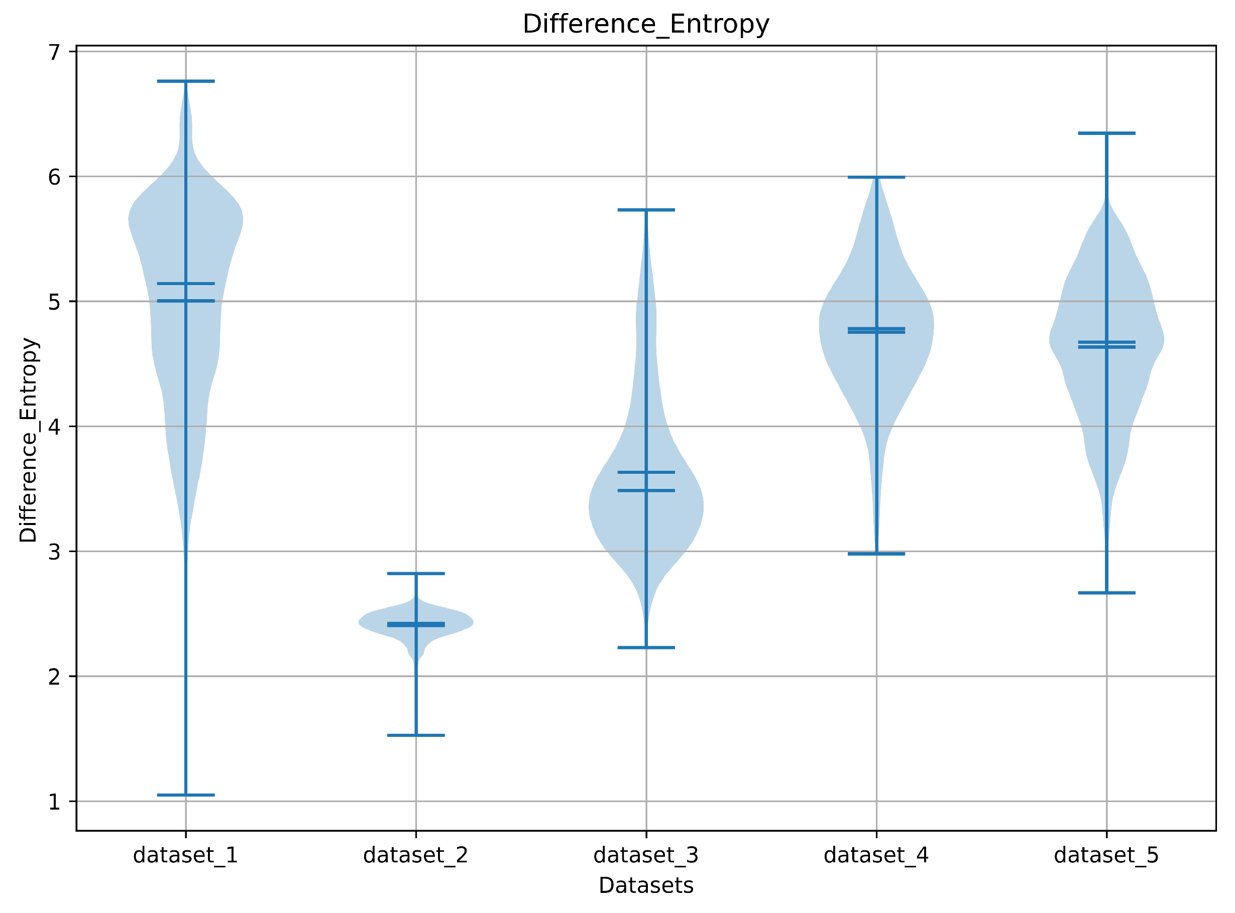
3.2.10. Difference Entropy

This reflects the randomness or unpredictability of the differences between adjacent pixel pairs. Figure 12 shows that dataset_2 has the lowest difference entropy value among the other datasets. It is computed using Equation (15):

$$\mathrm{Difference}\mathrm{Entropy}=\sum _{i=0}^{K-1}{P}_{(x-y)}\left(i\right)log\left\{P_{(x-y)}\left(i\right)\right\}$$

(15)

3.3. Highest-Lowest GLCM Metric’s Scorecard

Texture analysis for plant disease diagnosis relies heavily on image quality control and dataset selection criteria, as seen by the observed differences in GLCM metric scores between datasets. Although GLCM metrics were uniform and constant in certain datasets, they varied significantly in others, which can affect the validity of texture-based characteristics that were derived from the images. To distinguish between the performances of individual datasets, with regards to being the highest or lowest per metrics generated, the scorecard presented in

Table 3. GLCM metrics scorecard.

GLCM Metrics	Highest in GLCM					Lowest in GLCM
	1	2	3	4	5	1	2	3	4	5
Energy		x								x
Contrast	x				x		x
Correlation		x				x
Homogeneity		x				x
Angular Second Moment	x	x							x
Total Variance					x		x
Maximum Probability	x								x
Joint Entropy					x		x
Difference Variance					x		x
Difference Entropy	x						x
Sum of scores:	4	4	0	0	4	2	5	0	2	1

was developed. The dataset_3 images include high-resolution variations spanning from 2048 × 1152 to 1280 × 720 pixels, indicating that image resolution may have an impact on texture analysis results. While lower-resolution images may result in information loss and poorer texture differentiation, higher-resolution pictures may capture finer texture features, leading to more nuanced GLCM measurements.

Dataset_2 scored the highest overall performance while dataset_3 showed the lowest overall scores per GLCM metric. Differences in image acquisition settings, environmental factors, and disease severity may be the cause of variations in GLCM metrics such as energy, contrast, and homogeneity between the respective datasets. For example, texture properties in images from lab-based datasets 1 and 2 might be more consistent because the images were taken under controlled conditions, while field-based datasets 3, 4, and 5 (referring to Table 1) present more variability because of natural variations in plant physiology and environmental factors. This in turn calls for the need to conduct a more comprehensive analysis into the reasons why field-based datasets are lower in the GLCM metric score and whether this has an impact on machine/deep learning applications.

The observed discrepancies in the GLCM measure scores among datasets bear significant consequences for the robustness and generalizability of machine learning and deep learning models that are trained on these datasets. When compared to models trained on datasets with significant variability in texture qualities, models trained on datasets with consistent GLCM metrics might perform better and be more generalizable. The capacity of the model to identify discriminative patterns linked to various disease classes may be hampered by bias and noise introduced into the feature space by inconsistent GLCM metrics between datasets. In practical applications, this can result in less-than-ideal performance and decreased dependability, especially when used in varied and ever-changing agricultural settings.

3.4. Correlation Matrix of GLCM Metrics

To ascertain the relationships between individual GLCM metrics of these datasets, a correlation matrix was generated and is presented as a heatmap for easy visualization (Figure 13). The GLCM metrics were ordered in the following series: energy (1), contrast (2), correlation (3), homogeneity (4), angular second moment (5), total variance (6), maximum probability (7), joint entropy (8), difference variance (9), and difference entropy (10), respectively. With the use of the correlation matrix, the link between variables can be ascertained by calculating values between −1 and 1. Prior to developing any machine learning model, most data scientists believe that this is a decisive step as it helps determine which variables are most relevant for their model. Strongly correlated metrics appeared darker in color.

3.4.1. Strong Correlations

Energy and angular second moment: Higher values of energy are generally correlated with higher values of angular second moment, according to a strong positive correlation observed. In accordance with this, images with more uniform pixel values also tend to be more homogeneous. This has the potential to help machine learning algorithms to identify patterns or homogeneity in textures. Moreover, understanding this correlation is key for feature selection in image processing. Consequently, supposing either of the two metrics is highly representative, using both may not provide additional information.

Energy and maximum probability: The maximum probability of pixel pairs tends to grow as the uniformity (energy) of the image increases, due to a strong association observed. This indicates that more uniform plant disease images are likely to have a pixel pair that occurs more regularly than others. For machine learning and deep learning applications, this could impact tasks where the existence of specific pixel pairs is essential, such as in identifying unique texture patterns in certain diseases.

Maximum probability and angular second moment: There appears to be a considerable association between the likelihood of a certain pixel pair recurring frequently and the homogeneity of the image. This could mean that certain patterns or textures appear frequently and consistently across the image. For applications requiring a given texture pattern to occur frequently and to be uniform, such as diagnosing diseases based on recurring patterns, this will be worthwhile.

Joint entropy and difference entropy: A substantial positive correlation suggests that as the information content (joint entropy) of an image increases, the randomness in intensity differences (difference entropy) also increases. More information-rich images may show a wider range of intensity variations. This implies that the information content (joint entropy) of an image is related to the distribution of pixel intensities (maximum probability) classified within itself. Images with different distributions of pixel intensity could have more entropy. In terms of deep learning, this is valuable for tasks where understanding both the randomness in intensity differences and the overall information content is decisive, e.g., in tasks requiring diverse texture patterns.

3.4.2. Moderate Correlations

Contrast and joint entropy: According to the reasonable correlation between joint entropy and contrast, there tends to be a corresponding increase in the intensity difference between adjacent pixels (Contrast) as the individual plant disease image’s information content rises (greater joint entropy). This correlation further implies that images with higher entropy (more varied pixel pair intensities) also seem to have more noticeable contrasts in intensity between neighboring pixels.

This correlation may be useful for activities where it is important to understand both the overall information content and the fluctuations in local intensity. For example, it could be helpful to capture different texture patterns at the global and local levels in disease identification.

Contrast and difference entropy: A moderate link has been found between difference entropy and contrast, indicating that a rise in the unpredictability of intensity differences between pixels (higher difference entropy) is accompanied by an increase in the intensity difference between a pixel and its neighbors (contrast). According to this correlation, images with more diverse intensity differences between individual pixels also typically exhibit more pronounced intensity differences between neighboring pixels.

The effect on machine learning/deep learning applications could be linked to tasks where it is necessary to capture both the local changes in intensity and the global randomness in intensity differences. This correlation may aid in the identification of various texture patterns with unique local properties in the context of plant disease image analysis.

Correlation and homogeneity: A moderately positive correlation between these measures indicates that there is a tendency for a stronger correlation to be associated with higher homogeneity. This possibly will suggest, in the context of machine/deep learning, that textures with more homogeneity (homogeneity) shows a relationship with higher correlations between pixel values at various spatial distances, thus signifying a texture that is more predictable.

3.4.3. Weak Correlations

Difference entropy and difference variance: The low correlation seen between these metrics may suggest that the information contained in these differences (difference entropy) is not highly correlated with fluctuations in pixel differences across spatial distances (difference variance). This could imply, in terms of machine learning, that although pixel disparities vary, they may not significantly add to the image’s data content.

3.4.4. Inverse Correlation

Joint entropy and homogeneity: The negative correlation suggests that homogeneity and entropy are inversely proportional. That is to say, homogeneity seems to drop as joint entropy rises. This could imply that images tend to be less homogeneous when their entropy is larger. This may suggest that images with a wider range of pixel intensities have less homogeneity in machine learning.

3.4.5. Kruskal–Wallis Test of Variance

To find out whether there are statistically significant differences between the GLCM metrics, the Kruskal–Wallis test for non-parametric data was utilized. This is due to the datasets’ violation of ANOVA assumptions, including the normality of data and their hypotheses, as insights from the presented distribution of the parameters across the datasets portray. In this case, a statistical significance is indicated by a p-value less than 0.0001. Given the size of the datasets, the p-value is determined to be estimated rather than exact. Moreover, the multiple stars signify much more of the significance. It is true that there is a significant difference (p < 0.05) in the medians, as well, between the 10 GLCM metrics. Kress–Wallis Statistic value estimated as 619,192, which is given herein as the determined test statistic value.

In light of the findings summarized in

Table 4. Kruskal–Wallis Test.

Table Analyzed	GLCM 10 Parameters
p-value	<0.0001
Exact or approximate p-value?	Approximate
p-value summary	**** (Highly significant differences among the medians)
Do the medians vary significantly (p < 0.05)?	Yes
Number of groups	10
Kruskal–Wallis statistic	619,192
Data summary
Number of treatments (columns)	10
Number of values (total)	637,010

, machine/deep learning applications could be impacted owing to the significant differences in GLCM metrics across plant disease datasets, through the feature relevance of these metrics might be decisive in distinguishing plant diseases. Integrating these metrics through advanced modeling could significantly impact classification accuracy. Also, tailoring the deep learning or machine learning algorithms, as the case may be, to accommodate these differences has the potential to enhance their performance. Such algorithms could adapt their weights or learning rates based on the dataset’s specific characteristics shown by its GLCM metrics. Nevertheless, it will be crucial to understand which metrics vary significantly alongside the individual correlations between them. This will viably help allow targeted training through a fine-tuning style or separate training for each dataset, optimizing their analytical power for specific diseases.

Furthermore, metrics showing substantial unevenness or variations might correlate with disease severity. The severity of plant diseases based on image features will potentially help in accurately assessing these variations if properly leveraged. This could be true for enhancing the robustness of future machine learning and deep learning models, thus better handling diverse conditions and variations observed in different diseases.

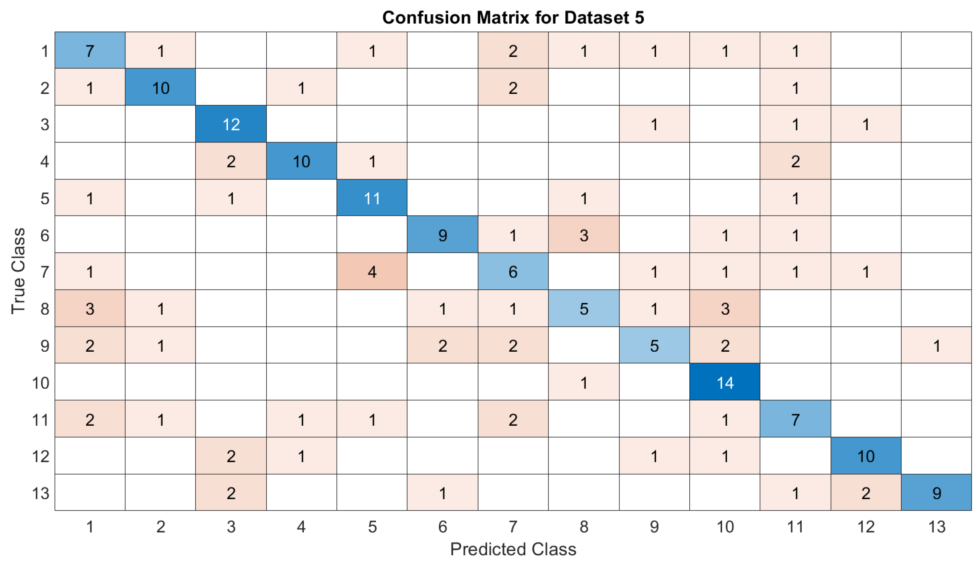
3.5. Deep Learning Model’s Development and Analysis

DarkNet19, a 19-layer deep convolutional neural network trained on more than a million images from the ImageNet database, was utilized for the detection of plant diseases. The pre-trained network can classify images into 1000 object categories, such as keyboard, mouse, pencil, and many animals. To maximize its performance, the model was trained through a number of epochs (10) that was kept fixed for the whole datasets used in this study. The training dataset was traversed entirely in each epoch, and the model’s parameters were updated using mini-batches of data throughout each iteration. To guarantee the best results, hyperparameters including learning rate, batch size, and regularization strategies were carefully adjusted. A general architecture of the DarkNet19 neural network is illustrated in Figure 14. For more detailed information on DarkNet19, please refer to [45].

As is known, the input data size significantly affects the model performance. Like other hyperparameters, the number of inputs should be the same for all data sets in order to make a fair evaluation. For this purpose, the class with the lowest number of samples was determined after all data sets were converted into separate image data stores with a Matlab code. Accordingly, the subclass labeled “Leamon (P10)_deseased” of D2 has the lowest number of image samples (77 images). Using this threshold value, 77 images were randomly selected from the subclasses of each dataset to obtain the final image datastore. Then, 80% of the data were randomly allocated for training and the remaining 20% for testing. The stages of preparing the datasets are shown in Figure 15. The results obtained from the deep learning training are presented in

Table 5. Testing performance metrics of the datasets in the deep learning.

Datasets	Accuracy	Precision	Recall	F1-Score
D1	0.9122	0.9141	0.9123	0.9111
D2	0.9060	0.9116	0.9061	0.9056
D3	0.6666	0.7329	0.6667	0.6411
D4	0.5866	0.5885	0.5867	0.5867
D5	0.5897	0.5996	0.5897	0.5852

. The average accuracy, precision, recall, and F1-score measures show differences in the deep learning models’ performance across the five datasets (D1–D5).

When training on the D1 and D2 datasets, the deep learning model demonstrated highly encouraging results on several assessment criteria, averaging 91.22% and 90.6% average testing accuracy, respectively. This suggests that there was a strong agreement between the models’ predictions and the ground truth labels for the test samples. The models’ capacity to properly classify diseased and healthy plant image samples while limiting false positives and false negatives was demonstrated by the average precision, recall, and F1-scores. The models found an effective compromise between accurately recognizing unhealthy plants (recall) and minimizing misclassifications (precision), as evidenced by the high values of average precision, recall, and F1-scores, respectively. Generally, when working with imbalanced datasets, the F1-score is very helpful as it provides a thorough assessment of the model’s overall performance by taking into account both precision and recall [22,46].

The training and validation metrics of DarkNet19 for dataset_2 are shown in Figure 16. As evidenced by the confusion matrix derived for D1 (Figure 17), 100% accuracy for 15 out of the 38 classes was recorded. The lowest was recorded as nine accurate predictions, thus indicating the suitability of both the dataset and model utilized (DarkNet19) since it has minimal errors. The average accuracy of D1 and D2 is higher than that of D3, D4, and D5, respectively, implying that in terms of accurately classifying disease classifications, the models trained on datasets D1 and D2 performed better overall.

The models trained on the D3, D4, and D5 datasets have difficulty with classification tasks, as evidenced by the decrease in accuracy scores found for these datasets. This could be because of inadequate representation of disease classes or perhaps the noise. Additionally, D1 and D2 have greater average precision values than D3, D4, and D5, suggesting that fewer false positives (misclassifications) occurred in the models trained on these datasets. As evidenced by the confusion matrix derived for D2 (Figure 18), a 100% accuracy for 7 out of the 22 classes was noted. The lowest was recorded as 11 accurate predictions, leaving four inaccurate classes, indicating the suitability and quality of the dataset for plant disease detection. The reduced precision values for D3, D4, and D5 point to an increased likelihood of false positives in the predictions, which caused much of the disease classes to be incorrectly identified (Figure 19, Figure 20 and Figure 21), indicating high accuracy in classifying the “disease” class but low performance in the case of “healthy” class. This made it clear that a low number of classes in the dataset is significant in its accuracy for deep learning applications.

When comparing models trained on D3, D4, and D5 to those trained on D1 and D2, the former showed greater average recall values, suggesting fewer false negatives (missed detections). The lower recall scores for D3, D4, and D5 indicate a higher proportion of false negatives, implying that the models may have failed to identify incidences of disease classes in the dataset.

The average F1-scores, which incorporate recall and precision, are greater for D1 and D2. This shows that the models trained on these datasets have a superior balance between precision and recall. The F1-score, in particular, suggests a good trade-off between precision and recall, which is considered essential for accurate disease detection [46]. It is possible that the class imbalances across these datasets are to blame for the lower F1-scores for D3, D4, and D5, which show a less-than-ideal balance between precision and recall.

4. Conclusions

In conclusion, this study explored the complex terrain of GLCM (Gray-Level Co-occurrence Matrix) metric changes in various plant disease datasets and concluded with a thorough investigation of their implications for deep learning applications in plant disease diagnosis. To shed light on the textural variations present, GLCM metrics were initially generated by carefully compiling a collection of plant images from five different disease datasets. Afterward, a number of meticulous statistical analyses were carried out to identify trends and variances in GLCM measures between the datasets, providing the foundation for wise choices in later phases of this research. Specifically, these analyses were used to assign scores to the datasets according to how well they performed on the GLCM measure, creating a quantitative standard for evaluating the quality of datasets.

Within the field of deep learning model building, our methodology stands out due to the careful synchronization with the understandings obtained from the GLCM analyses. Using the DarkNet19 architecture, each dataset was subjected to rigorous model training, with particular attention dedicated to validation and hyperparameter tuning. The trained models were thoroughly evaluated using performance indicators as benchmarks for the models/ability to identify plant diseases.

Most importantly, our results revealed a strong convergence between deep learning model performance and dataset quality as measured by GLCM measures. Of all the datasets analyzed, dataset_2 (D2) was identified as the best, as it had the highest GLCM scores and the best model performance metrics. This correspondence highlights how important dataset properties are, especially texture-based features that are captured by GLCM metrics, on the efficacy of deep learning models in plant disease detection. Significantly, this study emphasizes how important it is to have a discriminating criterion when choosing datasets for deep learning applications in plant disease detection in the future. The study further emphasizes the need for a comprehensive approach to dataset curation by comparing dataset quality indicators obtained from GLCM analysis with the results of subsequent deep learning model training. To ensure dataset compatibility and improve a model’s performance, this means going beyond conventional visual characteristics and including texture-based descriptors like GLCM metrics.

Overall, this work provides important new understandings of the complex interactions among dataset properties, GLCM measures, and deep learning model performance in plant disease identification. By promoting a thorough and discriminating approach to dataset selection, a door is hereby opened to better decision-making and increased effectiveness in future deep learning applications, pushing the boundaries of agricultural research and supporting initiatives for sustainable food production and global food security.

5. Recommendations and Future Works

In reference to the GLCM metric distribution across the datasets, the results emphasize how crucial it is to carry out a more thorough investigation in order to comprehend the fundamental causes of the variations in GLCM metric scores between datasets that are field- and lab-based. The possible effects of these variations on the effectiveness of deep learning or machine learning applications in the identification of plant diseases are also called into question. To improve texture analysis techniques’ resilience and dependability, as well as their use in practical situations, these issues might need to be resolved.

Owing to the limitations of this study in terms of generalization, the findings may be constrained by the specific plant disease datasets and deep learning methodologies employed. Generalizing the results to broader contexts, diverse plant classes, or other datasets deserves caution and further authentication.

Deep learning models trained in this work may not be as robust or generalizable due to the inherent biases and constraints of the chosen plant disease datasets, which include differences in image quality, disease severity, and class diversity. Acquiring datasets on plant diseases from multiple sources and repositories in order to encompass a wider range of plant species, diseases, and environmental factors will be a great development. Furthermore, to maintain consistency and comparability across various datasets, standardizing the procedures for acquiring such images, annotating them, and curating the data is recommended. This entails developing standards for camera settings, illumination, image resolution, and disease severity rating.

The incorporation of multispectral imaging techniques may allow for the acquisition of spectral information beyond the visible spectrum, thereby improving disease detection capacities and resilience to environmental variability.

Future research could investigate the integration of other texture descriptors, such as Gabor filters or Local Binary Patterns (LBPs), in addition to the GLCM metrics that were the focus of our study on texture analysis. This multi-modal method could lead to improved model performance by offering a more thorough analysis of texture features in plant disease images.

Improving model generalizability and guaranteeing dependable performance across various imaging conditions and illness scenarios requires addressing dataset biases and variability in texture features. To improve the accuracy and dependability of automated plant disease detection systems, future research should concentrate on creating strong feature extraction techniques and model architectures that can adjust to changes in textural characteristics and environmental factors.

References

1. FAO. The State of Food and Agriculture, 1974. Lancet 1975, 306, 313–314. [Google Scholar] [CrossRef]
2. FAO. FAO—News Article: New Standards to Curb the Global Spread of Plant Pests and Diseases; Food and Agriculture Organization of the United Nations: Roma, Italy, 2018. [Google Scholar]
3. Horst, R.K. Plant Diseases and Their Pathogens. In Westcott’s Plant Disease Handbook; Springer: Berlin/Heidelberg, Germany, 2001; pp. 65–530. [Google Scholar] [CrossRef]
4. FAO. International Year of Plant Health—Final Report; FAO: Rome, Italy, 2021. [Google Scholar] [CrossRef]
5. Buja, I.; Sabella, E.; Monteduro, A.G.; Chiriacò, M.S.; De Bellis, L.; Luvisi, A.; Maruccio, G. Advances in plant disease detection and monitoring: From traditional assays to in-field diagnostics. Sensors 2021, 21, 2129. [Google Scholar] [CrossRef] [PubMed]
6. Strange, R.N.; Scott, P.R. Plant Disease: A Threat to Global Food Security. Annu. Rev. Phytopathol. 2005, 43, 83–116. [Google Scholar] [CrossRef] [PubMed]
7. Witten, I.H.; Cunningham, S.; Holmes, G.; McQueen, R.J.; Smith, L.A. Practical Machine Learning and its Potential Application to Problems in Agriculture. In Practical Machine Learning and Its Potential Application to Problems in Agriculture; Department of Computer Science, University of Waikato: Hamilton, New Zealand, 1993; Volume 1, pp. 308–325. [Google Scholar]
8. Shrivastava, V.K.; Pradhan, M.K. Rice plant disease classification using color features: A machine learning paradigm. J. Plant Pathol. 2021, 103, 17–26. [Google Scholar] [CrossRef]
9. Zhou, H.; Li, Y.; Zhang, Q.; Xu, H.; Su, Y. Soft-sensing of effluent total phosphorus using adaptive recurrent fuzzy neural network with Gustafson-Kessel clustering. Expert Syst. Appl. 2022, 203, 117589. [Google Scholar] [CrossRef]
10. Lecun, Y.; Bengio, Y.; Hinton, G. Deep learning. Nature 2015, 521, 436–444. [Google Scholar] [CrossRef] [PubMed]
11. Tibdewal, M.N.; Kulthe, Y.M.; Bharambe, A.; Farkade, A.; Dongre, A. Deep Learning Models for Classification of Cotton Crop Disease Detection. Zeich. J. 2022, 8. [Google Scholar]
12. Prakash, N.; Udayakumar, E.; Kumareshan, N. Design and development of Android based Plant disease detection using Arduino. In Proceedings of the 2020 7th International Conference on Smart Structures and Systems, ICSSS 2020, Chennai, India, 23–24 July 2020. [Google Scholar] [CrossRef]
13. Petchiammal, A.; Briskline Kiruba, S.; Murugan, D. Paddy Leaf diseases identification on Infrared Images based on Convolutional Neural Networks. arXiv 2022, arXiv:2208.00031. [Google Scholar] [CrossRef]
14. Ahmad, A.; Saraswat, D.; El Gamal, A. A survey on using deep learning techniques for plant disease diagnosis and recommendations for development of appropriate tools. Smart Agric. Technol. 2023, 3, 100083. [Google Scholar] [CrossRef]
15. Hughes, D.P.; Salathe, M. An open access repository of images on plant health to enable the development of mobile disease diagnostics. arXiv 2015, arXiv:1511.08060. [Google Scholar]
16. Pardede, H.F.; Suryawati, E.; Zilvan, V.; Ramdan, A.; Kusumo, R.B.S.; Heryana, A.; Yuwana, R.S.; Krisnandi, D.; Subekti, A.; Fauziah, F.; et al. Plant diseases detection with low resolution data using nested skip connections. J. Big Data 2020, 7, 57. [Google Scholar] [CrossRef]
17. Thakur, P.S.; Sheorey, T.; Ojha, A. VGG-ICNN: A Lightweight CNN model for crop disease identification. Multimed. Tools Appl. 2023, 82, 497–520. [Google Scholar] [CrossRef]
18. Nagi, R.; Tripathy, S.S. Plant disease identification using fuzzy feature extraction and PNN. Signal Image Video Process. 2023, 17, 2809–2815. [Google Scholar] [CrossRef]
19. Hanh, B.T.; Van Manh, H.; Nguyen, N.V. Enhancing the performance of transferred efficientnet models in leaf image-based plant disease classification. J. Plant Dis. Prot. 2022, 129, 623–634. [Google Scholar] [CrossRef]
20. Wiesner-Hanks, T.; Stewart, E.L.; Kaczmar, N.; Dechant, C.; Wu, H.; Nelson, R.J.; Lipson, H.; Gore, M.A. Image set for deep learning: Field images of maize annotated with disease symptoms. BMC Res. Notes 2018, 11, 440. [Google Scholar] [CrossRef] [PubMed]
21. Barbedo, J.G.A. Impact of dataset size and variety on the effectiveness of deep learning and transfer learning for plant disease classification. Comput. Electron. Agric. 2018, 153, 46–53. [Google Scholar] [CrossRef]
22. Pérez-Enciso, M.; Zingaretti, L.M. A Guide for Using Deep Learning for Complex Trait Genomic Prediction. Genes 2019, 10, 553. [Google Scholar] [CrossRef]
23. Singh, D.; Jain, N.; Jain, P.; Kayal, P.; Kumawat, S.; Batra, N. PlantDoc: A dataset for visual plant disease detection. In Proceedings of the ACM International Conference Proceeding Series, Association for Computing Machinery, Dhaka, Bangladesh, 10–12 January 2020; pp. 249–253. [Google Scholar] [CrossRef]
24. Oyewola, D.O.; Dada, E.G.; Misra, S.; Damaševičius, R. Detecting cassava mosaic disease using a deep residual convolutional neural network with distinct block processing. Peerj Comput. Sci. 2021, 7, e352. [Google Scholar] [CrossRef] [PubMed]
25. Parraga-Alava, J.; Cusme, K.; Loor, A.; Santander, E. RoCoLe: A robusta coffee leaf images dataset for evaluation of machine learning based methods in plant diseases recognition. Data Brief 2019, 25, 104414. [Google Scholar] [CrossRef]
26. Zhang, X.; Han, L.; Dong, Y.; Shi, Y.; Huang, W.; Han, L.; González-Moreno, P.; Ma, H.; Ye, H.; Sobeih, T. A Deep Learning-Based Approach for Automated Yellow Rust Disease Detection from High-Resolution Hyperspectral UAV Images. Remote Sens. 2019, 11, 1554. [Google Scholar] [CrossRef]
27. Bhakta, I.; Phadikar, S.; Majumder, K. Thermal Image Augmentation with Generative Adversarial Network for Agricultural Disease Prediction. In Lecture Notes in Networks and Systems; Springer Science and Business Media Deutschland GmbH: Berlin/Heidelberg, Germany, 2022; Volume 480, pp. 345–354. [Google Scholar] [CrossRef]
28. Mohanty, S.P.; Hughes, D.P.; Salathé, M. Using deep learning for image-based plant disease detection. Front. Plant Sci. 2016, 7, 215232. [Google Scholar] [CrossRef] [PubMed]
29. Chen, M.; French, A.P.; Gao, L.; Ramcharan, A.; Hughes, D.P.; Mccloskey, P.; Baranowski, K.; Mbilinyi, N.; Mrisho, L.; Ndalahwa, M.; et al. A Mobile-Based Deep Learning Model for Cassava Disease Diagnosis. Front. Plant Sci. 2019, 10, 272. [Google Scholar] [CrossRef]
30. Johannes, A.; Picon, A.; Alvarez-Gila, A.; Echazarra, J.; Rodriguez-Vaamonde, S.; Navajas, A.D.; Ortiz-Barredo, A. Automatic plant disease diagnosis using mobile capture devices, applied on a wheat use case. Comput. Electron. Agric. 2017, 138, 200–209. [Google Scholar] [CrossRef]
31. Ahmad, J.; Jan, B.; Farman, H.; Ahmad, W.; Ullah, A. Disease detection in plum using convolutional neural network under true field conditions. Sensors 2020, 20, 5569. [Google Scholar] [CrossRef]
32. Petchiammal; Kiruba, B.; Murugan; Arjunan, P. Paddy Doctor: A Visual Image Dataset for Automated Paddy Disease Classification and Benchmarking. In Proceedings of the 6th Joint International Conference on Data Science and Management of Data (10th ACM IKDD CODS and 28th COMAD), Mumbai, India, 4–7 January 2023; pp. 203–207. [Google Scholar] [CrossRef]
33. Mikołajczyk, A.; Grochowski, M. Data augmentation for improving deep learning in image classification problem. In Proceedings of the 2018 International Interdisciplinary PhD Workshop, IIPhDW 2018, Swinoujscie, Poland, 9–12 May 2018; pp. 117–122. [Google Scholar] [CrossRef]
34. Velásquez, A.C.; Castroverde, C.D.M.; He, S.Y. Plant–Pathogen Warfare under Changing Climate Conditions. Curr. Biol. 2018, 28, R619–R634. [Google Scholar] [CrossRef] [PubMed]
35. Wang, Q.; He, G.; Li, F.; Zhang, H. A novel database for plant diseases and pests classification. In Proceedings of the ICSPCC 2020—IEEE International Conference on Signal Processing, Communications and Computing, Proceedings, Macau, China, 21–24 August 2020. [Google Scholar] [CrossRef]
36. Gadkari, D. Image Quality Analysis Using GLCM. In Electronic Theses and Dissertations; University of Central Florida: Orlando, FL, USA, 2004; pp. 1–120. [Google Scholar]
37. Hall-Beyer, M. Practical guidelines for choosing GLCM textures to use in landscape classification tasks over a range of moderate spatial scales. Int. J. Remote Sens. 2017, 38, 1312–1338. [Google Scholar] [CrossRef]
38. Mall, P.K.; Singh, P.K.; Yadav, D. GLCM based feature extraction and medical X-RAY image classification using machine learning techniques. In Proceedings of the 2019 IEEE Conference on Information and Communication Technology, CICT 2019, Allahabad, India, 6–8 December 2019. [Google Scholar] [CrossRef]
39. Kadir, A. A Model of Plant Identification System Using GLCM, Lacunarity And Shen Features. Publ. Res. J. Pharm. Biol. Chem. Sci. 2014, 5, 1–10. [Google Scholar]
40. Shoaib, M.; Shah, B.; EI-Sappagh, S.; Ali, A.; Ullah, A.; Alenezi, F.; Gechev, T.; Hussain, T.; Ali, F. An advanced deep learning models-based plant disease detection: A review of recent research. Front. Plant Sci. 2023, 14, 1158933. [Google Scholar] [CrossRef] [PubMed]
41. Gupta, H.P.; Chopade, S.; Dutta, T. Computational Intelligence in Agriculture. In Emerging Computing Paradigms; John Wiley and Sons, Ltd.: Hoboken, NJ, USA, 2022; pp. 125–142. [Google Scholar] [CrossRef]
42. Wang, G.; Sun, Y.; Wang, J. Automatic Image-Based Plant Disease Severity Estimation Using Deep Learning. Comput. Intell. Neurosci. 2017, 2017, 2917536. [Google Scholar] [CrossRef]
43. Barbedo, J.G.A.; Koenigkan, L.V.; Halfeld-Vieira, B.A.; Costa, R.V.; Nechet, K.L.; Godoy, C.V.; Junior, M.L.; Patricio, F.R.A.; Talamini, V.; Chitarra, L.G.; et al. Annotated plant pathology databases for image-based detection and recognition of diseases. IEEE Lat. Am. Trans. 2018, 16, 1749–1757. [Google Scholar] [CrossRef]
44. Barbedo, J.G. Factors influencing the use of deep learning for plant disease recognition. Biosyst. Eng. 2018, 172, 84–91. [Google Scholar] [CrossRef]
45. Redmon, J. Darknet: Open Source Neural Networks in C. 2013–2016. Available online: http://pjreddie.com/darknet/ (accessed on 16 May 2024).
46. Theodoridis, S. Machine Learning: A Bayesian and Optimization Perspective, 2nd ed.; Academic Press: Cambridge, MA, USA, 2020; pp. 1–1131. [Google Scholar] [CrossRef]
Figure 1. The stages of the proposed methodology.
Electronics 13 02299 g001
Figure 2. The representation of GLCM calculation.
Electronics 13 02299 g002
Figure 3. GLCM metrics: energy.
Electronics 13 02299 g003
Figure 4. GLCM metrics: contrast.
Electronics 13 02299 g004
Figure 5. GLCM metrics: correlation.
Electronics 13 02299 g005
Figure 6. GLCM metrics: homogeneity.
Electronics 13 02299 g006
Figure 7. GLCM metrics: angular second moment.
Electronics 13 02299 g007
Figure 8. GLCM metrics: total variance.
Electronics 13 02299 g008
Figure 9. GLCM metrics: maximum probability.
Electronics 13 02299 g009
Figure 10. GLCM metrics: difference variance.
Electronics 13 02299 g010
Figure 11. GLCM metrics: joint entropy.
Electronics 13 02299 g011
Figure 12. GLCM metrics: difference entropy.
Electronics 13 02299 g012
Figure 13. Correlation matrix of the derived GLCM metrics.
Electronics 13 02299 g013
Figure 14. The architecture of the DarkNet19 neural network.
Electronics 13 02299 g014
Figure 15. The stages of preparing final datasets with equal class-image numbers.
Electronics 13 02299 g015
Figure 16. Training and validation metrics for dataset_2.
Electronics 13 02299 g016
Figure 17. Confusion matrix for dataset_1.
Electronics 13 02299 g017
Figure 18. Confusion matrix for dataset_2.
Electronics 13 02299 g018
Figure 19. Confusion matrix for dataset_3.
Electronics 13 02299 g019
Figure 20. Confusion matrix for dataset_4.
Electronics 13 02299 g020
Figure 21. Confusion matrix for dataset_5.
Electronics 13 02299 g021