A Surrogate Model for the Rapid Evaluation of Electromagnetic-Thermal Effects under Humid Air Conditions

Abstract

Integrated circuits are being more and more extensively applied, and the reliability issues of devices are receiving increased attention from researchers. The study of electronic device performance is not limited to the device themselves; these studies also need to consider the operating environment, such as high temperature or high humidity, which requires fluid simulation. However, this approach inevitably increases the complexity of modeling and the difficulty of the equations to be solved. Aiming at the simulation of the thermal performance of a device under coupled humid air conditions, this paper proposes a surrogate model to quickly evaluate the multiphysical effects of humid air and a multiphysical solver based on it. In this research, the finite element method (FEM) is utilized to simulate the multiphysical problem, and the proposed method is verified as being efficient.

1. Introduction

Recent decades have witnessed the rapid development of the integrated circuit industry and the vigorous growth of fields such as unmanned autonomous driving, high-speed supercomputing, and automated production lines. In the context of these large-scale applications, the reliability [1,2,3] of electric equipment during operation is receiving considerable attention; this issue refers to the ability to accomplish designed objectives within the expected life span despite various operating conditions. It is worth noting that solely focusing on the electromagnetic performance of a device is no longer enough to meet the aforementioned requirements. For chips and other thermal-sensitive devices, thermal field changes in the circuit or devices also affect electromagnetic performance [4,5,6,7]. Specifically, the Joule heating effect generated by the interconnects becomes increasingly significant with increasing duration of operation [8]. Such heat accumulation not only elevates the operating temperature of the entire circuit, leading to instability in its operational state, but also leads to overheating in local areas within the device [9]. Significant temperature gradients can also induce thermal stresses, posing the risks of breakage and the solder failure of the device. Therefore, thermal reliability issues are particularly prominent. In this case, if the electromagnetic field and temperature are still solved independently during the simulation, it inevitably leads to significant deviation from the practical performance. Therefore, it is necessary to analyze multiphysical problems in actual working scenarios.

Researchers have proposed various methods to analyze multiphysical problems [10,11,12,13] in the operation of electric devices. The numerical method is commonly employed for solving multiphysics problems due to its accurate calculation and fine simulation of the model’s structure [14,15,16]. Nevertheless, the work mentioned above shares a limitation: the influence of humid air on the device was not considered. Given that devices can work on rainy or windy days, the fluid field composed of the surrounding humid air also couples with the thermal field, acting together on electronic devices [17,18,19]. Therefore, it is essential to consider the coupling effects of electromagnetics, heat, and humid air to contribute to improving the accuracy of modeling and simulation for the entire system.

Efforts have also been made to couple humid air with thermal field calculations. As the noncondensable gas in the surrounding vapor has a significant influence on condensation heat transfer, researchers [20] developed a coupled transient multiphysics solver to investigate droplet condensation in a moist air environment. Authors [21] adopted computational fluid dynamics (CFD) simulation to predict the combined fluid flow and transfer phenomena in the steady state for a humid cavity and compared the results with those obtained from experiments. The general trends, experimentally observed, were well predicted, while some differences still existed, indicating that the simulation was not accurate enough. In [22], a model for heat and moisture transport in porous materials was proposed to take the effect of indoor air distributions into account when simulating the hygric response of porous objects. This method is more accurate but has poor scalability and may have a higher computational cost because different models need to be established for different material properties and then coupled in a 3D CFD simulation. An equivalent circuit [23] was used to simulate the response of the moisture inside power electronics, which consisted of variable and controlled resistors and capacitors to describe the diffusivity, permeability, and storage in polymers. But, this approach involves equivalent circuit modeling for each heating part and water diffusion path in the structure, which results in a substantial workload and is not convenient or fast. Researchers [24] adopted neural networks to predict air temperature and humidity at the outlet of a wire-on-tube-type heat exchanger. However, this method relies on a large number of preliminary experiments to establish the dataset, which means a large time cost and manual work.

In this paper, a simpler and more reliable method is proposed to calculate the electromagnetic and thermal effects of humid air coupling conditions on electronic devices. We simulated the multiphysical performance of the whole device. The rest of this paper is organized as follows: Firstly, Section 2 introduces the thermal–fluid coupling method and proposes an approximation method using the equivalent convection heat transfer coefficient, instead of solving the fluid–structure interaction equation. Then, Section 3 analyzes the mechanism and specific process of electric–thermal–fluid field coupling and provides a numerical example to verify the developed multiphysics simulation solver. Finally, the conclusions are presented in Section 4.

2. Theory and Methodology

The impacts of humid air on electronic products mainly include condensation, diffusion, and adsorption. However, with existing packaging technologies, the components have been observed to absorb little moisture from the external environment. Additionally, the packaging structure also has good moisture resistance, and little corrosion or damage occurs to the internal circuits of the chip due to vapor intrusion. Therefore, the water vapor in humid air has little impact on the electromagnetic performance of a circuit. On this premise, this paper only considers the thermal effects when including humid air in multiphysics coupling.

2.1. Finite Element Method for Electricity and Heat Transfer

Numerical simulation is a typical method of analyzing the physical performance of a device under the coupled effects of electricity, heat, and humidity. Following this approach, researchers need to construct a precise and comprehensive model of the entire electronic device structure, as well as the intricate interconnections within, and then perform appropriate meshing according to structural characteristics [25,26]. In this study, we assumed that the electronic device generates heat due to the Joule heat effect during operation, and then we analyzed its temperature distribution of the under humid air. In the literature [27], a nonuniform rectangular grid finite volume method (FVM) was used to solve the voltage distribution equation and heat equation of solid media and fluid flow. In the literature [28], electromagnetic analysis was achieved using the discontinuous Galergin time domain (DGTD) method, and the thermal analysis was realized via the finite element time-domain (FETD) method.

In this study, we used the FEM, and the electric field distribution was calculated by solving the current continuity equation rather than Maxwell equations because the current continuity equation is more suitable for solving static and quasi-static problems, and it simplifies the computational complexity. It is well suited for the problems discussed in this paper and effectively incorporates the boundary conditions of the electrical potential. The governing equations used are shown below:

$$\nabla ·[\sigma \left(T\right)·\nabla U]=\frac{\partial \rho \left(t\right)}{\partial t}$$

(1)

$${\left.U\right|}_{\Gamma \mathrm{a}}=\overline{U}$$

(2)

$${\left.\frac{\partial U}{\partial n}\right|}_{\Gamma \mathrm{q}}=-{\left.\frac{J}{\sigma \left(T\right)}\right|}_{\Gamma \mathrm{q}}$$

(3)

where the variable T denotes the temperature and the parameter t means time. The variable $\sigma \left(T\right)$ is the material conductivity that changes with its temperature T and the fitting formula is shown in Equation $\left(4\right)$ [29], where the coefficients are listed in

Table 1. Coefficients in the electrical conductivity expression.

Coefficient	Value
$A_0$	2.9115 × 108
$A_1$	−1.5643 × 106
$A_2$	3.7000 × 103
$A_3$	−3.9347
$A_4$	−1.5644 × 10−3

:

The variable U represents the transient electric potential and $\rho \left(t\right)$ denotes the volume charge density. In equation $\left(2\right)$, the variable $\overline{U}$ indicates the voltage on the first type of boundary, which can load the external electromagnetic pulse. The parameter n represents the normal direction outside the boundary and the parameter J is the volume current density entering vertically on the boundary.

$$\sigma \left(T\right)=\sum _{i=0}^4{A}_{\mathrm{i}}{T}^{\mathrm{i}},200\mathrm{K}\le T\le 900\mathrm{K}$$

(4)

When thermal field analysis takes into account the wet environment, humid air is the medium of fluid heat transfer, while solid heat transfer occurs inside the electronic devices, so it is necessary to consider the heat transfer problem in such a fluid–structure interaction. Then, the corresponding governing equations to be solved are as follows [30]:

$$\frac{\partial \rho }{\partial t}+\nabla ·\left(\rho ·\overrightarrow{V}\right)=0$$

(5)

$$\rho \frac{\partial \overrightarrow{V}}{\partial t}+\rho (\overrightarrow{V}·\nabla )\overrightarrow{V}+\nabla p=\mu ·{\nabla }^2\overrightarrow{V}+\overrightarrow{F}$$

(6)

$$\rho C_p\frac{\partial T}{\partial t}+\rho C_p\overrightarrow{V}·\nabla T=\lambda {\nabla }^{2}T+Q$$

(7)

where the variables $\rho$, $\overrightarrow{V}$, p, $\mu$, $C_{\mathrm{p}}$ and $\lambda$ respectively denote the density, velocity vector, pressure, dynamic viscosity, specific heat capacity and thermal conductivity of the humid air. The variables $\overrightarrow{F}$ and Q represent the volume force exerted on the fluid and heat generation or absorption of a unit volume.

Obviously, compared with the current continuity equation mentioned above, it is difficult to solve these equations since they are composed of one first-order partial differential equation and two second-order partial differential equations. Moreover, fine modeling with a huge number of nodes and elements inevitably leads to large numbers of matrix equations. Both factors mentioned ultimately result in considerable computation and time costs. In order to simplify the model as much as possible, this paper proposes an equivalent method. This method calculates the heat transfer coefficient h between the packaged chip and the outside environment for the real-time temperature, humidity, and flow rate of humid air. The coupled thermal effects between the humid air and the interconnect circuit is equivalently represented by a heat transfer coefficient. This method avoids directly solving the complicated partial differential equations but instead focuses on the heat transfer characteristics of the fluid–solid boundary at different temperatures by updating the key parameters of the surrounding humid air. Theoretically, the method greatly reduces the complexity of the solver and saves computing resources.

Based on the equivalent method, the governing equations for the thermal problem in this study can be simplified as follows:

$$\begin{array}{c}\rho c\frac{\partial T}{\partial t}=\nabla ·(\lambda \nabla T)+f(T,t)\end{array}$$

(8)

$$\begin{array}{c}{\left.T\right|}_{\Gamma \mathrm{a}}=\overline{T}\end{array}$$

(9)

$$\begin{array}{c}{\left.\widehat{n}·(\lambda \nabla T)\right|}_{\Gamma \mathrm{q}}=-{\left.h\left(T-T_a\right)\right|}_{\Gamma \mathrm{q}}\end{array}$$

(10)

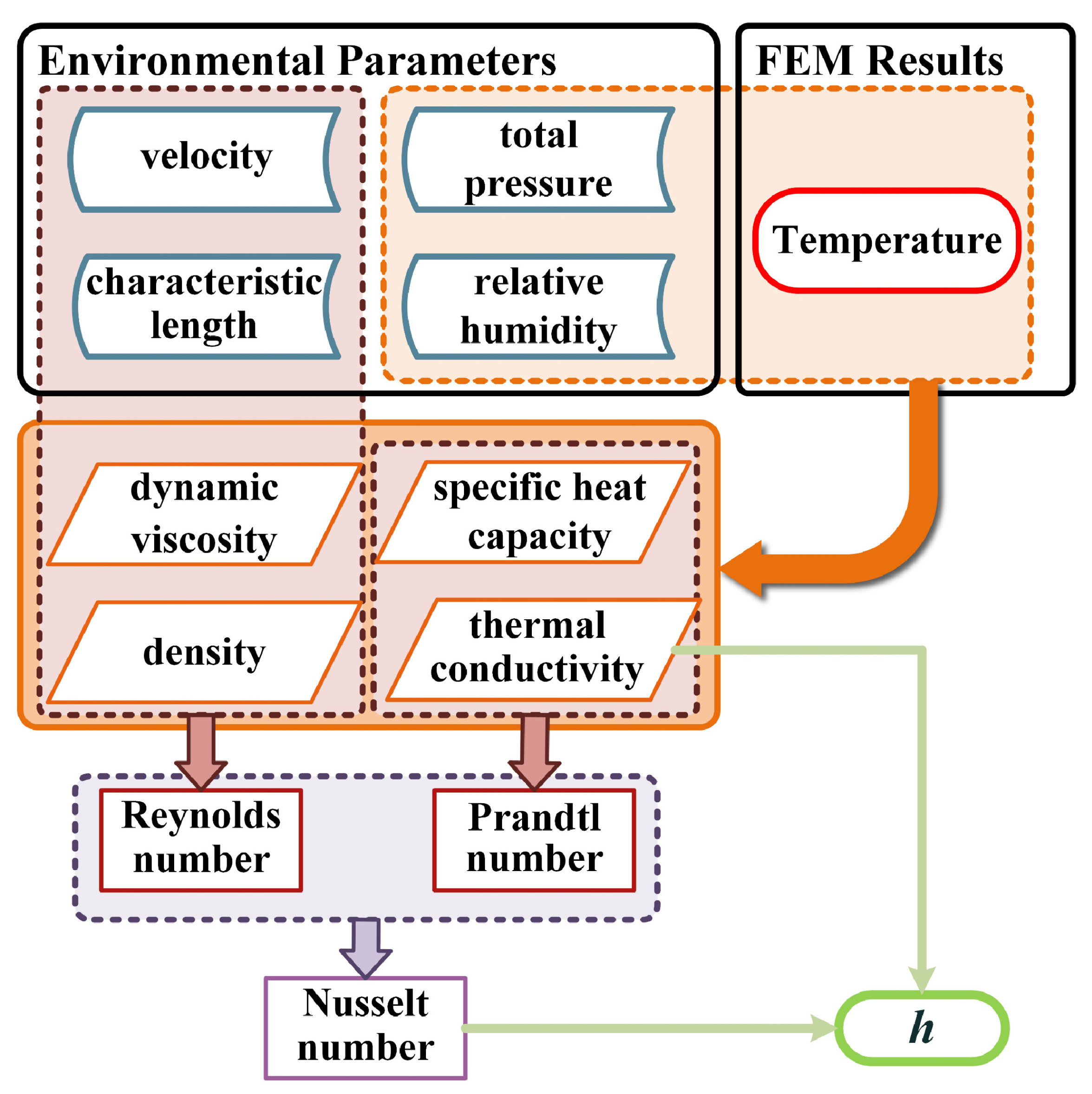
2.2. Derivation of Equivalent Convective Heat Transfer Coefficient

In order to take the humid air into account in a simpler way, this study choses the equivalent convective heat transfer coefficient h as the medium, and we coupled the humid air outside and inside the electronic device by updating the temperature and physical parameters of humid air with the change in this coefficient. Humid air is regarded as a mixture of dry air and pure vapor, and the thermal properties of humid air can be calculated based on the physical properties of these two components. For convenience, the physical quantities mentioned in the following text are distinguished by different subscripts, where the subscript $\mathrm{ma}$, $\mathrm{da}$ and $\mathrm{v}$ represent humid air that we are interested in, dry air and vapor, respectively. The specific derivation and calculation process is shown in Figure 1.

This figure depicts that only basic environmental parameters such as the flow rate, relative humidity, atmospheric pressure, and initial temperature of humid air need to be known to calculate the key thermal physical parameters of the fluid and ultimately obtain the convective heat transfer coefficient. In this paper, the electrical–thermal coupling primarily manifests in the influence of circuit operation on chip structure temperature and the effect of temperature variations on material conductivity. Therefore, the value of temperature T is the object of the finite element solution. The following provides a detailed derivation and calculation of the equivalent convective heat transfer coefficient h.

The moisture content of humid air d could be calculated with the following formula:

$$\begin{array}{c}d=\frac{622·\phi p_{\mathrm{s}}\left(T\right)}{p_{\mathrm{ma}}-\phi p_{\mathrm{s}}\left(T\right)}\end{array}$$

(11)

where the parameter $p_{\mathrm{ma}}$ is the total pressure of humid air, and the parameter $p_{\mathrm{s}}\left(T\right)$ is the saturation pressure of vapor which varies with the temperature of humid air. The variable $\phi$ is the relative humidity, which could be obtained through on-site measurements.

The density of humid air can be calculated as

$$\begin{array}{c}{\rho }_{\mathrm{ma}}=\frac{p_{\mathrm{ma}}(1+0.001·d)}{R_{\mathrm{da}}T(1+0.001606·d)}\end{array}$$

(12)

where the parameter $R_{\mathrm{da}}$ is the gas constant of dry air, usually taken as 287 $\mathrm{J}/\left(\mathrm{kg}·\mathrm{K}\right)$.

The dynamic viscosity of humid air could be obtained as the function of ${\mu }_{\mathrm{da}}$ and ${\mu }_{\mathrm{v}}$, the dynamic viscosity of dry air and vapor. This function is shown as

$$\begin{array}{c}{\mu }_{\mathrm{ma}}=\frac{M_{\mathrm{da}}^{-\frac{1}{2}}{\mu }_{\mathrm{da}}+d{M}_{\mathrm{v}}^{-\frac{1}{2}}{\mu }_{\mathrm{v}}}{M_{\mathrm{da}}^{-\frac{1}{2}}+d{M}_{\mathrm{v}}^{-\frac{1}{2}}}\end{array}$$

(13)

where the parameter $M_{\mathrm{da}}$ is the molecular weight of dry air, taken as 28.97 and the parameter $M_{\mathrm{v}}$ is the molecular weight of vapor, taken as 18.02.

The following formula presents the specific heat capacity of wet air at constant pressure:

$$\begin{array}{c}{c}_{p,\mathrm{ma}}=\frac{c_{p,\mathrm{da}}+d·c_{p,\mathrm{v}}}{1+d}\end{array}$$

(14)

The thermal conductivity of humid air is related to not only the thermal conductivity of its components (vapor and dry air) but also the dynamic viscosity and molecular weight of the components. The formula can be listed as

$$\begin{array}{c}{\lambda }_{\mathrm{ma}}=\frac{{\lambda }_{\mathrm{da}}}{1+d\frac{M_{\mathrm{da}}}{M_{\mathrm{v}}}{A}_{\mathrm{da},\mathrm{v}}}+\frac{d{\lambda }_{\mathrm{v}}}{d+\frac{{\mu }_{\mathrm{v}}}{{\mu }_{\mathrm{da}}}{A}_{\mathrm{da},\mathrm{v}}}\end{array}$$

(15)

where the parameter $A_{\mathrm{da},\mathrm{v}}$ is the binding factor of dry air and water vapor.

$$\begin{array}{c}{A}_{\mathrm{da},\mathrm{v}}=\frac{{\left[1+{\left(\frac{{\mu }_{\mathrm{da}}}{{\mu }_{\mathrm{v}}}\right)}^{\frac{1}{2}}·{\left(\frac{M_{\mathrm{v}}}{M_{\mathrm{da}}}\right)}^{\frac{1}{4}}\right]}^2}{{\left[8·\left(1+\frac{M_{\mathrm{da}}}{M_{\mathrm{v}}}\right)\right]}^{-\frac{1}{2}}}\end{array}$$

(16)

The flow state, together with the density, velocity, dynamic viscosity, and characteristic length of the fluid passing through the object, forms a dimensionless parameter known as the Reynolds number. The expression is as follows:

$$\begin{array}{c}Re=\frac{{\rho }_{\mathrm{ma}}·v·L}{{\mu }_{\mathrm{ma}}}\end{array}$$

(17)

The Prandtl number is also a dimensionless quantity, and the expression is as follows:

$$\begin{array}{c}Pr=\frac{{\mu }_{\mathrm{ma}}·c_{\mathrm{p},\mathrm{ma}}}{{\lambda }_{\mathrm{ma}}}\end{array}$$

(18)

The formula that defines the Nusselt number is

$$\begin{array}{c}Nu=\frac{h·L}{\lambda }\end{array}$$

(19)

For different fluid states and geometric characteristics of objects, the specific value of the Nusselt number is calculated via appropriate empirical correlations. The correlation formula used in this study is listed as follows:

$$\begin{array}{c}Nu=2·\frac{0.3387·{(Re)}^{\frac{1}{2}}·{(Pr)}^{\frac{1}{3}}}{{\left[1+{\left(\frac{0.0468}{Pr}\right)}^{\frac{2}{3}}\right]}^{\frac{1}{4}}}\end{array}$$

(20)

According to Equation (19), the expression for the equivalent convective heat transfer coefficient h can be derived as follows:

$$\begin{array}{c}h=\frac{Nu·{\lambda }_{ma}}{L}\end{array}$$

(21)

From the previous derivation, it can be inferred that the convective heat transfer coefficient h is a function of temperature T, relative humidity $\varphi$, flow velocity v of humid air, and atmospheric pressure p. During a certain period of time, the relative humidity $\varphi$, the flow rate v, and the atmospheric pressure p of humid air can all be regarded as constants and do not change: due to the subtle heat dissipation and sharp temperature changes, they are usually confined to a very small region surrounding the electronic device. Therefore, in this study, the environmental parameters such as relative humidity $\varphi$, flow velocity v, and atmospheric pressure p remained unchanged during the numerical calculation process. That is, during the simulation, the value of the equivalent convective heat transfer coefficient h was updated simply with changes in temperature T. The values of the other parameters are specified at the beginning of the simulation.

Based on the previous derivation, the control equation can be transformed to

$$\begin{array}{c}\left\{\begin{array}{c}\rho c\frac{\partial T}{\partial t}=\nabla ·(\lambda \nabla T)+f(T,t)\\ {\left.T\right|}_{\Gamma \mathrm{a}}=\overline{T}\\ \widehat{n}·(k\nabla T)=-h(\phi ,p,v,T)·\left(T-T_{\mathrm{a}}\right)\end{array}\right.\end{array}$$

(22)

In the equation above, the convective heat transfer coefficient h is no longer a fixed value but a variable related to relative environmental humidity $\varphi$, atmospheric pressure p, fluid velocity v, and temperature T. With the introduction of an equivalent coefficient h, the originally complex and challenging fluid–structure interaction problem is simplified into a solid heat transfer problem. The fluid heat transfer is calculated with boundary conditions, which results in reduced modeling effort and simplified problem solving.

2.3. Multiphysics Coupling Mechanism

This section describes the general coupling mechanism of the multiphysical field problem. The purpose of electrical calculation is to obtain the electric field distribution of the chip interconnect circuit. Before the electrical simulation, it is imperative to declare the boundary conditions, such as whether there is a constant voltage boundary or a time-varying boundary condition, the type of excitation source, and how the excitation source is involved in the calculation. After the these preprocessing operations, the electrical problem can be solved to obtain the electric potential and electric field distribution. The next step is to solve the thermal problem. Similarly, the relevant conditions such as initial temperature and the other thermal parameters of the surrounding air should also be declared first. It is noticeable that the external heat source comes from the Joule heat generated by the operating of the circuit. The formula is expressed as

$$\begin{array}{c}f(T,t)=J·E=\sigma (T,t)·E^2\end{array}$$

(23)

In this case, the right term in the heat conduction equation is closely related to the electrical solver. In the electrical problem, the electrical conductivity of the material changes with temperature, while in the thermal problem, the external heat source is obtained via electrical analysis and is the Joule heat generated by the circuit.

The electric FEM solver should transmit the updated heat source data to the thermal solver after each iteration. Also, after every iteration of the thermal FEM solver, it is necessary to transmit the latest real-time temperature back to the electric FEM solver and update the convective heat transfer coefficient h and material conductivity $\sigma$. The temperature T and Joule heat obtained from each iteration of the electric–thermal multiphysics computation should to be reintroduced into the whole program and form a new cycle until the a converged result is acquired.

3. Numerical Validation

The FEM solver in this study adopted a three-dimensional tetrahedral element in the geometry splitting process, which is convenient to conform various structures. We selected COMSOL Multiphysics software Version 6.1, developed by COMSOL Inc., Burlington, MA 01803, USA, for validation.

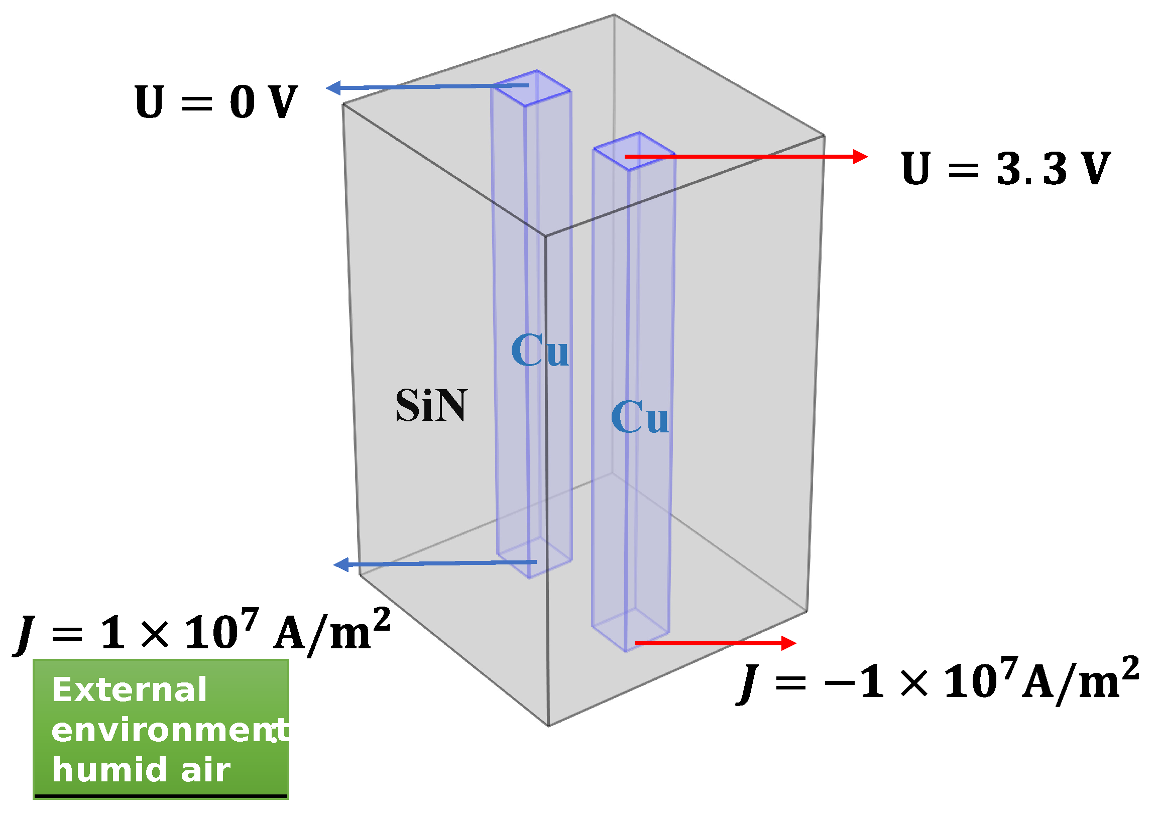
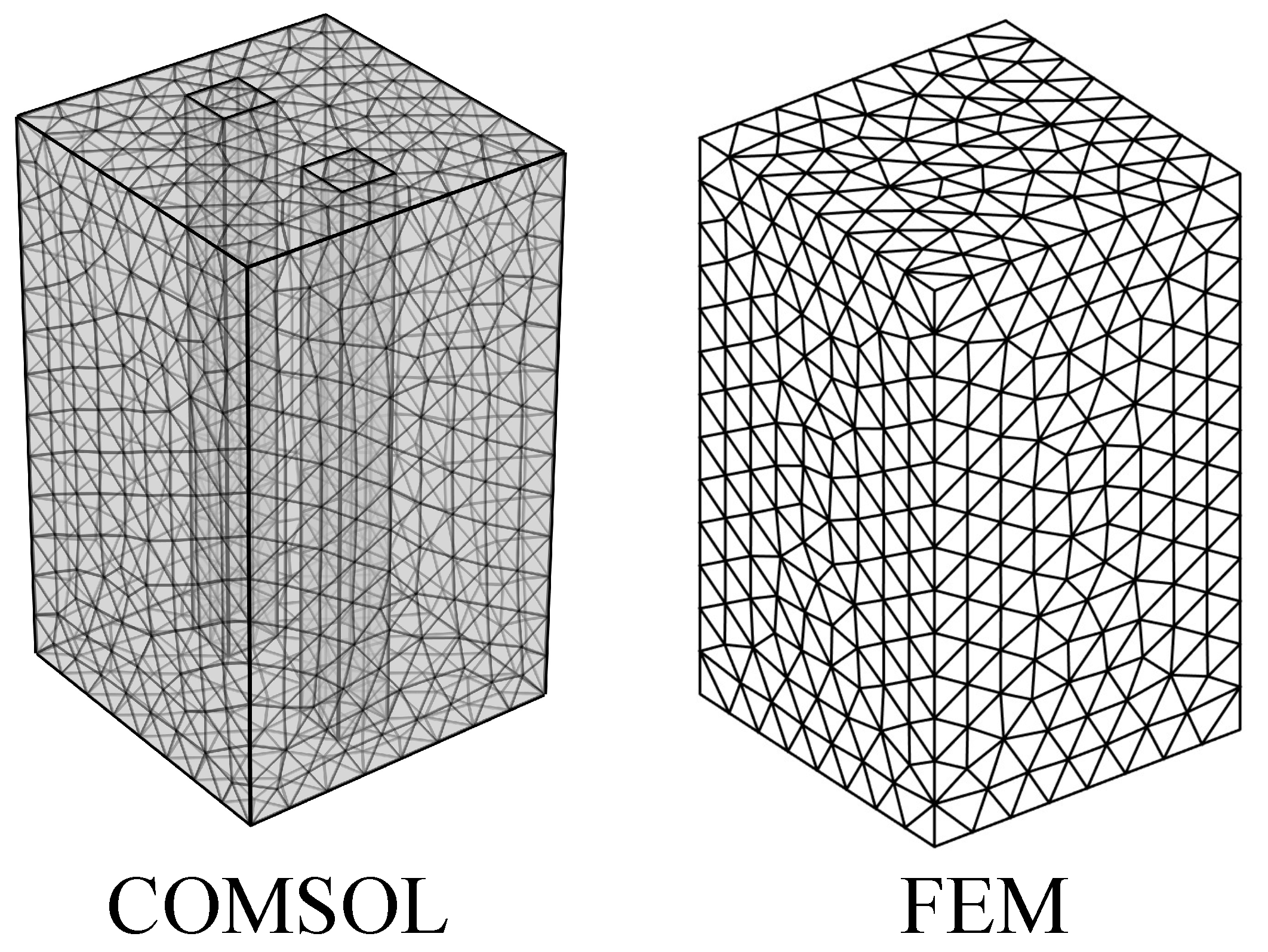
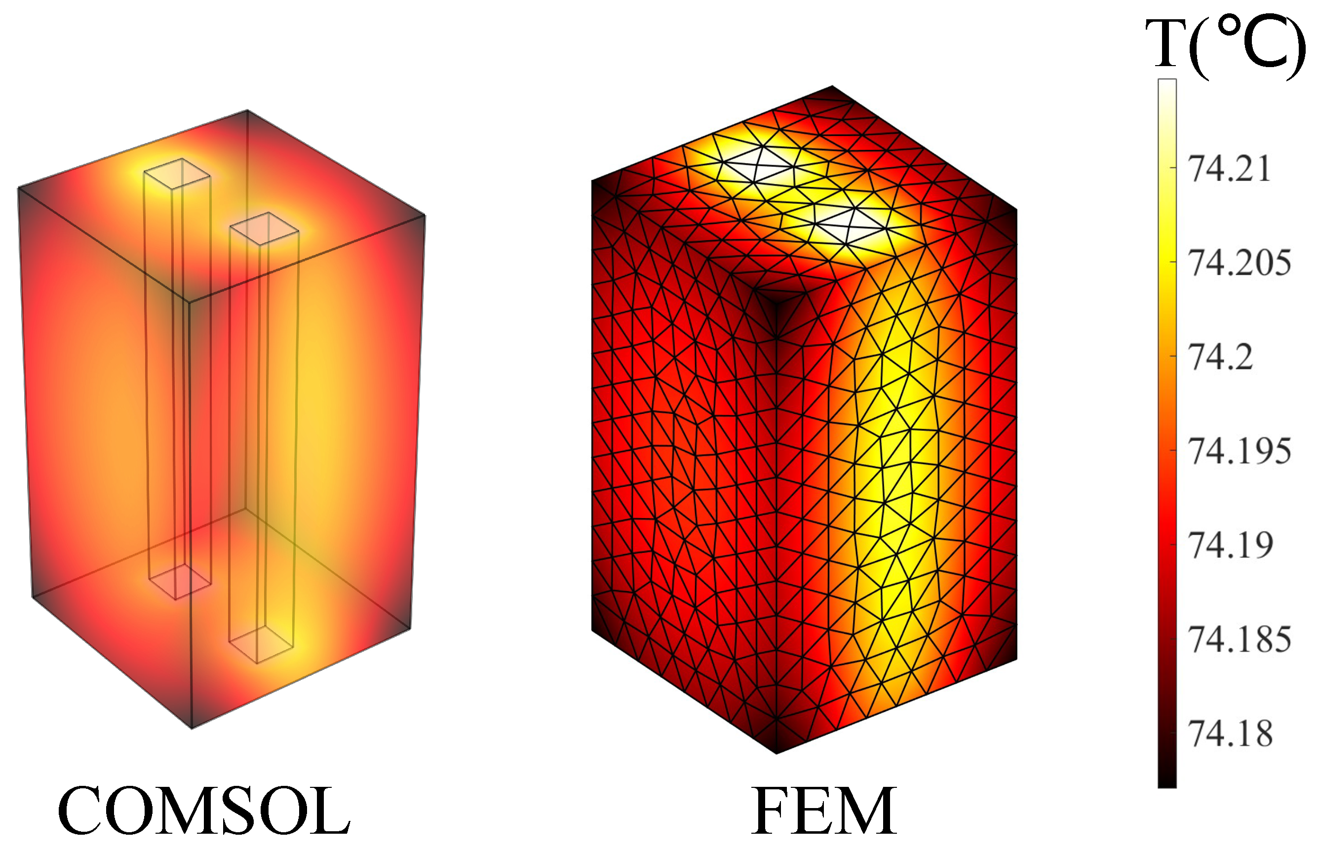
3.1. Case1: A Dual-Conductor Model Fully Encased within SiN

Assume that there is a 6 $\mathrm{mm}$ × 6 $\mathrm{mm}$ × 10 $\mathrm{mm}$ rectangle made of SiN with two copper conductor rods embedded, the sizes of which are both 1 $\mathrm{mm}$ × 1 $\mathrm{mm}$ × 10 $\mathrm{mm}$. The external environment is a fluid field composed of humid air. The flow direction of the humid air is perpendicular to the side of the rectangular body, sweeping across the geometry, as shown in Figure 2. Voltage sources are added to the upper surfaces of the copper conductor rods, while volume current density flows into the rods from the bottom, working as the current source excitation. For the left copper conductor, the upper surface voltage is 0, and the normal current density is 1 × 10⁷ $\mathrm{A}/{\mathrm{m}}^2$. For the other, the upper surface voltage is 3.3 $\mathrm{V}$, and the normal current density is −1 × 10⁷ $\mathrm{A}/{\mathrm{m}}^2$. The copper and SiN parameters are listed in

Table 2. Parameters of materials.

Material	Cu	SiN
$\sigma$$(\mathrm{S}/\mathrm{m})$	5.80 × 107	0
C $(\mathrm{J}/(\mathrm{kg}·\mathrm{K}\left)\right)$	3.85 × 102	7.00 × 102
$\rho$$(\mathrm{kg}/{\mathrm{m}}^3)$	7.90 × 103	3.00 × 103
$\lambda$$(\mathrm{W}/(\mathrm{m}·\mathrm{K}\left)\right)$	3.83 × 102	2.00 × 102

:

In this example, the characteristics of the fluid field were set as follows: the relative humidity was 50%, the atmospheric pressure was one standard atmospheric pressure (101,325 $\mathrm{Pa}$), and the external temperature was 66.85 °C. The initial temperature of the rectangular structure was 26.85 °C. The meshed used in FEM and Comsol are depicted in Figure 3, and the temperature distributions obtained from the coupling calculation of the electric–thermal–fluid field and COMSOL are shown in Figure 4.

In general, the results of the FEM solver and COMSOL are identical. In order to compare the calculation errors more accurately, we laid a domain point probe inside the cuboid and observed the temperature change over the simulation time. The curves are drawn in Figure 5.

It is obvious that the calculation results of the FEM are consistent with those of COMSOL despite some slight differences during the initial stages, and the outcome agrees well when the temperature reaches a plateau. Notably, the fluid velocity here is 0.1 $\mathrm{m}/\mathrm{s}$, which is relatively slow, and humid air is almost still, so we repeated the simulation above at a fluid velocity of 0.5 $\mathrm{m}/\mathrm{s}$ and 2 $\mathrm{m}/\mathrm{s}$ to be obtain more information. The results are presented in Figure 6 and Figure 7.

With the increase in the flow rate, as can be seen from the curves above, the time cost for the device to reach the steady-state temperature is lower. The rising trend and steady-state values of the temperature calculated with the FEM solver are consistent with those from COMSOL, except for slight differences in the initial stage. The relative error curve in Figure 8 also provides a powerful proof.

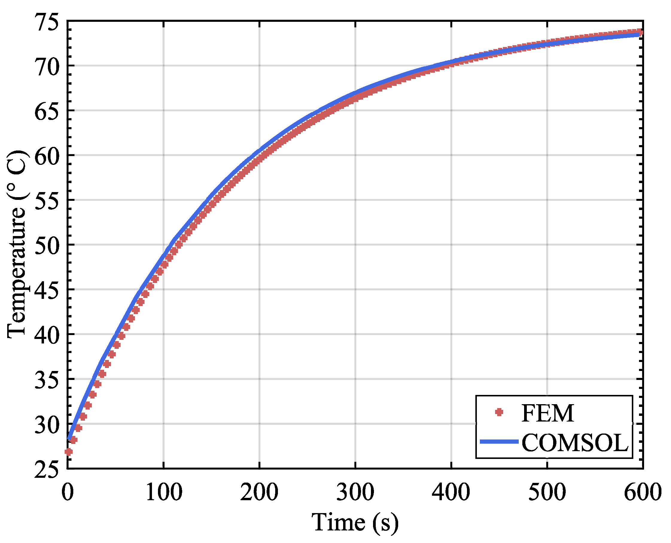
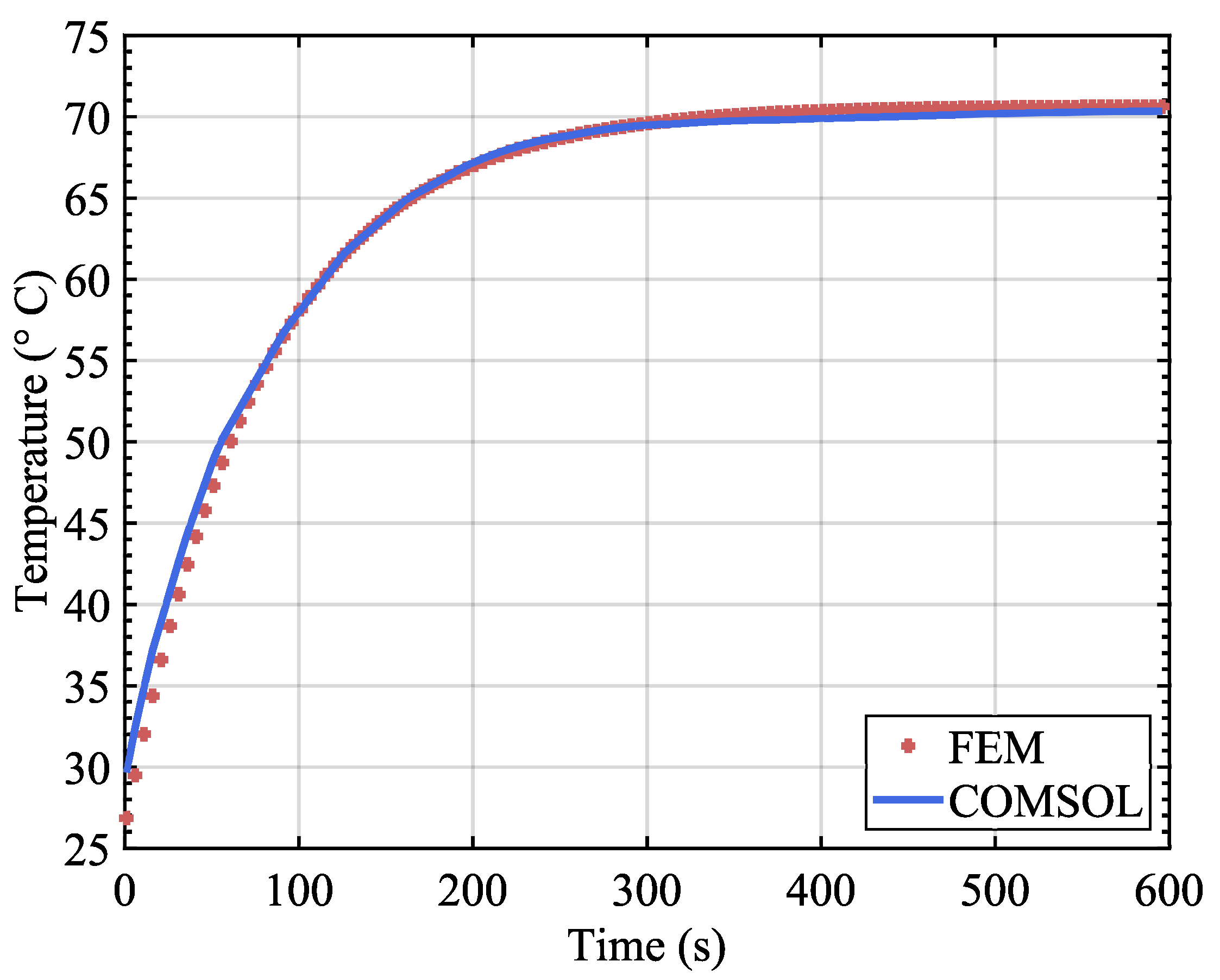
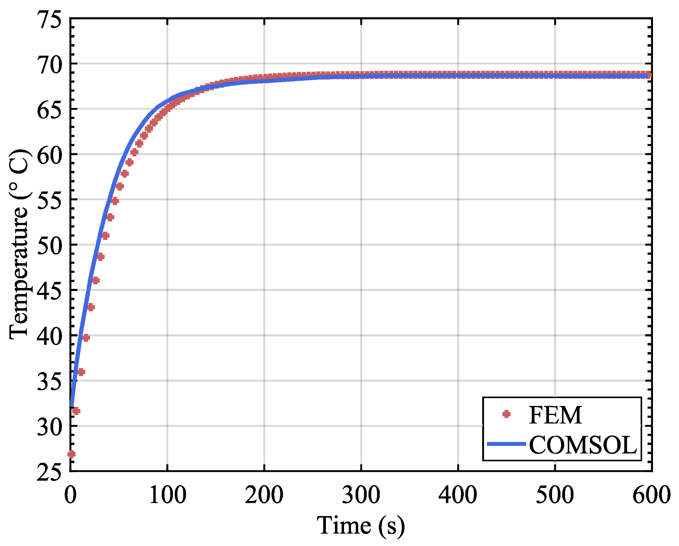
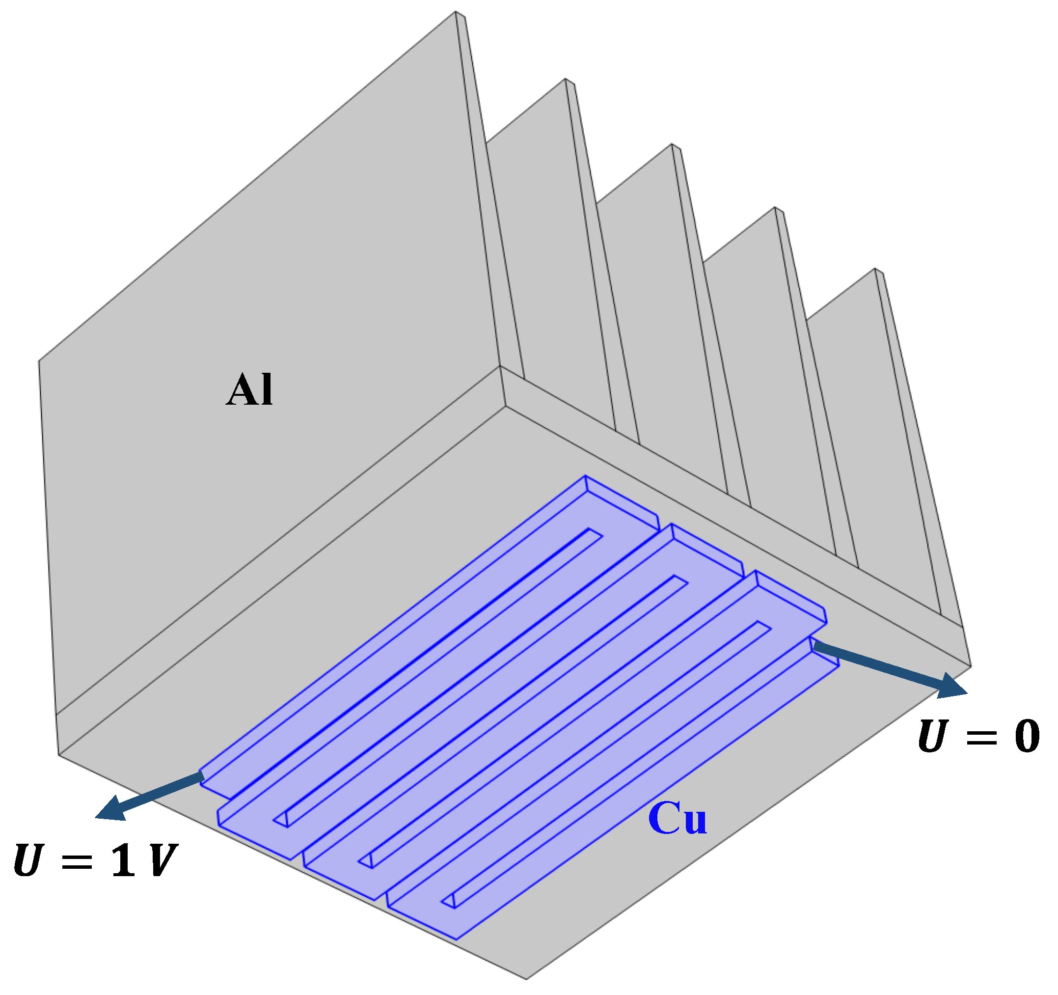
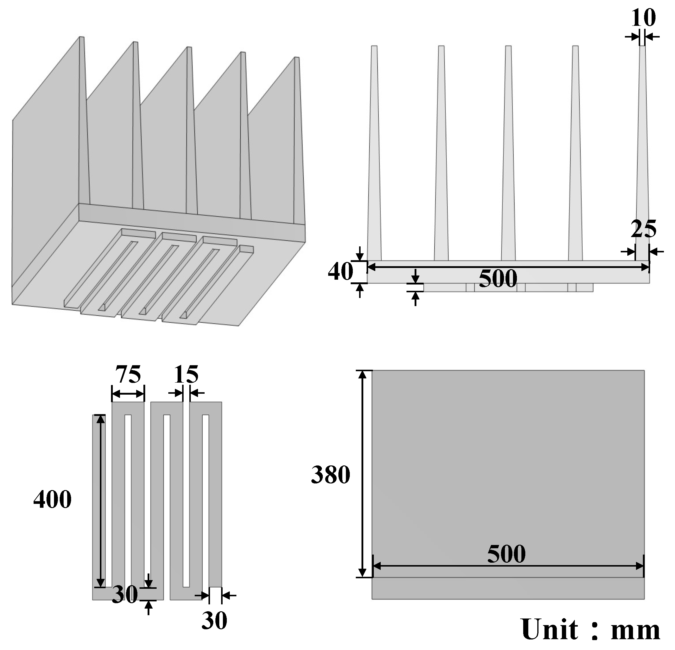
3.2. Case2: A Five-Finned Heat Sink Heated by a Serpentine Rail

In the previous model, the conductors were completely wrapped inside the SiN, and thus the internal heat dissipation was constrained by SiN. To demonstrate the algorithm’s general applicability, two more models with various cooling methods and diverse geometric structures provide a comprehensive evaluation of our algorithm’s effectiveness. In this section, we discuss a heat sink with five fins and an electrically heated rail in contact with its bottom, as shown in Figure 9. Its geometric parameters are indicated in Figure 10. In this case, the heat sink is made of aluminum with a side length of 0.5 $\mathrm{m}$, and the rail is still made of copper. The two ends of the rail are excited with different voltages, as identified in the figure. The parameters of the fluid field were set as follows: the relative humidity was 50 %, the fluid velocity was 1 $\mathrm{m}/\mathrm{s}$, the atmospheric pressure was one standard atmospheric pressure (101,325 $\mathrm{Pa}$), and the external temperature and initial temperature of the model are both 26.85 °C.

Different from the previous case, there are two main ways for the heat dissipation of the powered track in this model. Firstly, it is the convective heat dissipation between the surface of the rail and the surrounding humid air. The other is that the heat is conducted to the heat sink through the adjacent surface in close contact with the snake-shaped electric heating track. Then the heat exchange is realized between the multiple fins of the heat sink and the surrounding environment. Due to the superior thermal conductivity of metal compared with humid air, the heat sink assists in increasing the surface area for convective heat dissipation, thereby enhancing the heat dissipation efficiency. In this case, the meshes used for FEM and Comsol are displayed in Figure 11. The temperature distribution of this example obtained from the coupling calculation of the electric-thermal-fluid field and COMSOL is shown in Figure 12 and Figure 13 presents the temperature curve and relative error curve of a probe inside the structure to display a more accurate comparison of the results. This model proves the adaptability and accuracy of the proposed algorithm under different heat dissipation modes.

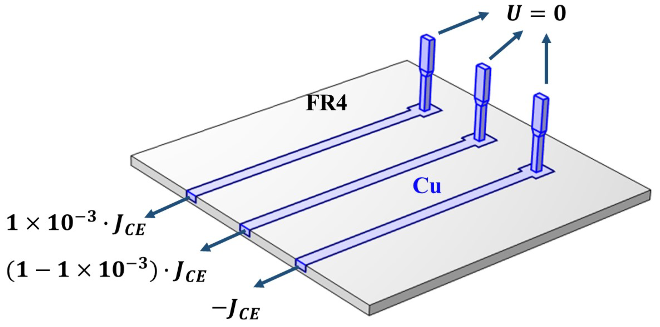
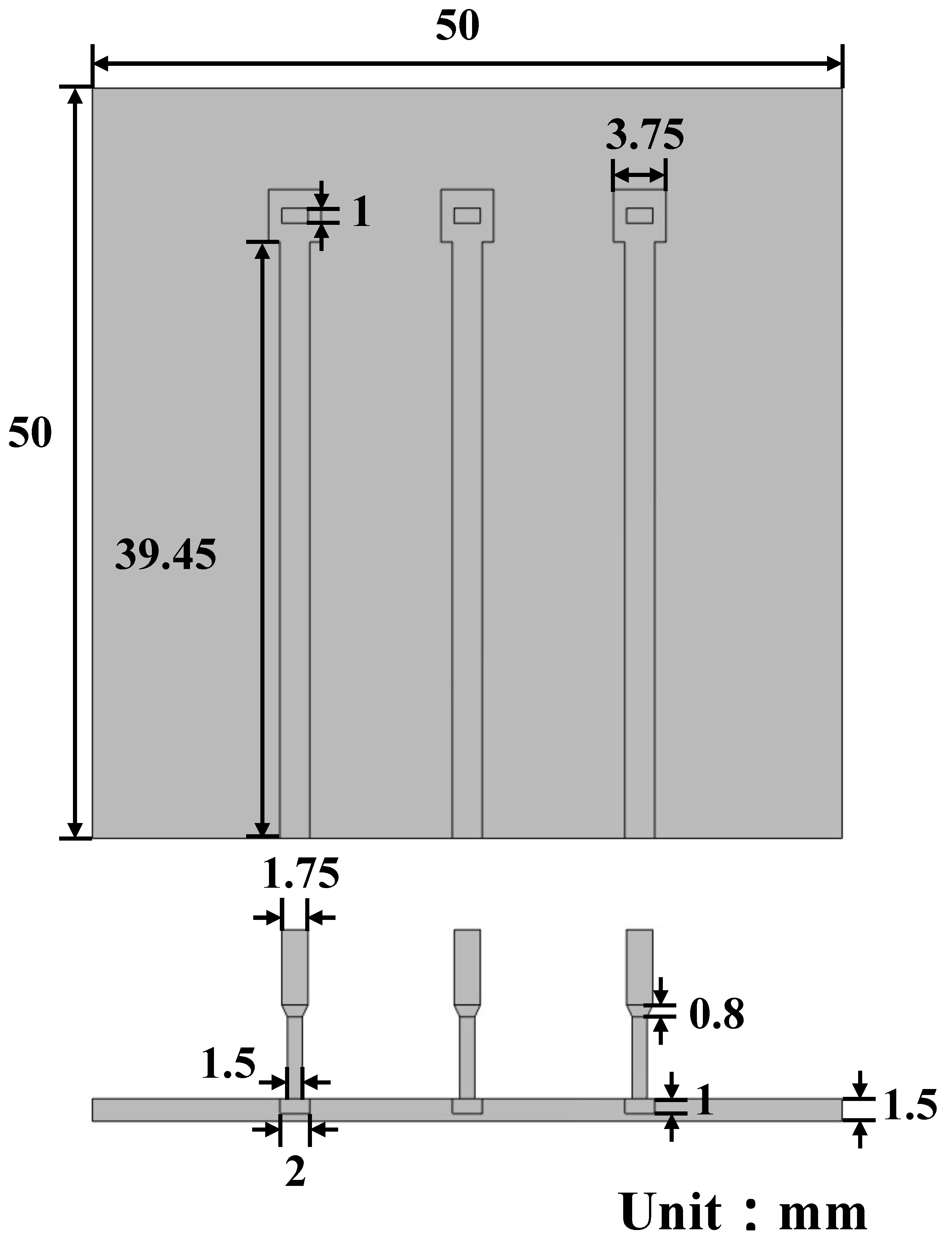
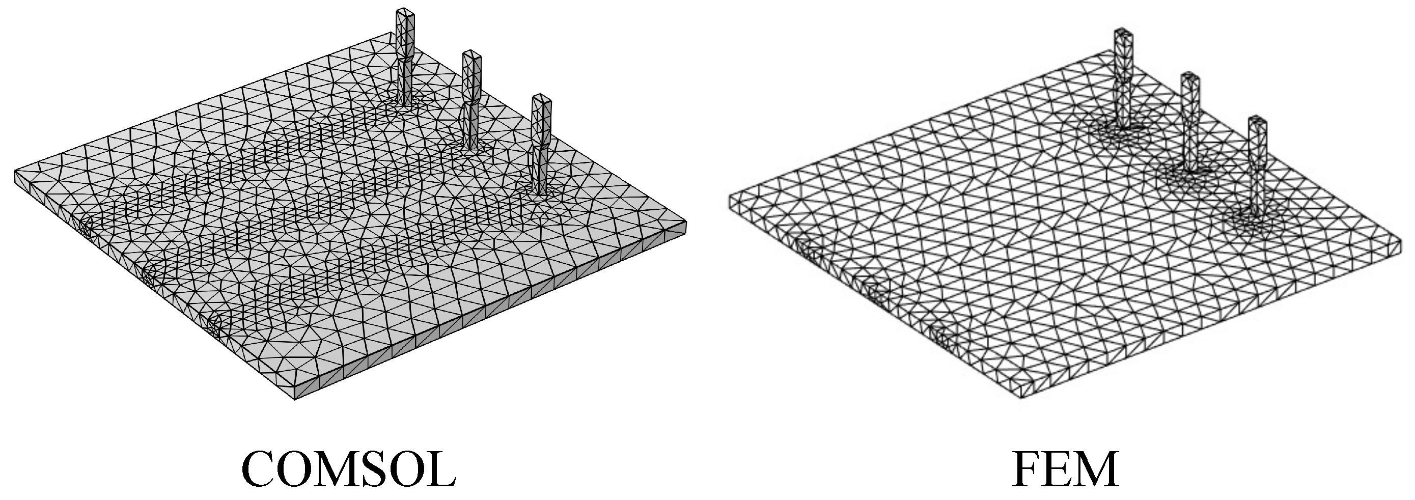
3.3. Case3: Power Transistor Pins Partially Embedded into the Substrate

The last case to be simulated had a more elaborate structure. It was composed of a nonconductive FR4 substrate and conductive metal, including three pins of a power transistor and a conductive layer embedded in the substrate. The structure and boundary conditions are clearly indicated in Figure 14; notably, $J_{CE}$ here is 3 × 10⁷ $\mathrm{A}/{\mathrm{m}}^2$. The geometric parameters of this case are highlighted in Figure 15.

Similarly, the pins here are still made of copper, while the substrate is almost nonconductive and adiabatic. The external temperature and initial temperature of the model are both 20.85 °C, while the other environmental parameters are the same as those in the five-finned heat sink with a serpentine rail. The different meshes used in FEM and Comsol are presented in Figure 16. The temperature distributions from FEM and COMSOL for the pins and the substrate are presented in Figure 17. The temperature curve and relative error curve of a probe inside the structure are illustrated in Figure 18. The results indicate that the proposed algorithm is applicable to various structures involving coupled electrical–thermal–humid-air phenomena, and could provide accurate and reliable predictions for trends in temperature distribution and increases.

The discussion above demonstrates the computational accuracy of the algorithm, and the following table provides strong support for its reduced computational resource consumption.

Table 3. Memory usage.

	FEM	COMSOL	Memory Saved
Case 1	1.32 G	2.11 G	37.4%
Case 2	1.33 G	2.53 G	47.4%
Case 3	0.68 G	2.39 G	71.5%

compares the memory usage of this algorithm with that of COMSOL. It is obvious that this algorithm has great advantages in reducing the consumption of computing resources, as expected, regardless of the structural features.

4. Conclusions

For the purpose of simplifying the solution to fluid–structure interaction heat transfer problems, this article proposed an equivalent convective heat transfer coefficient h, which represents the instant characteristics of humid air, and then we included the fluid through boundary conditions. The results compared with those from the commercial software COMSOL indicated that this method can simultaneously achieve accurate calculations and significantly save memory usage. To summarize, this method was proven to effectively reduce the complexity of modeling and the computational workload of simulation while achieving satisfactory accuracy.

References

1. Sravan, K.M.; Sachin, S.S. A holistic analysis of circuit performance variations in 3-D ICs with thermal and TSV-induced stress considerations. IEEE Trans. Very Large Scale Integr. VLSI Syst. 2015, 23, 1308–1321. [Google Scholar]
2. Arvind, R.S.; Alessandro, V.; Martino, R.; Thomas, B.; David, A. 3D-ICE: Fast compact transient thermal modeling for 3D ICs with inter-tier liquid cooling. In Proceedings of the 2010 IEEE/ACM International Conference on Computer-Aided Design (ICCAD), San Jose, CA, USA, 7–11 November 2010; pp. 463–470. [Google Scholar]
3. Wang, Y.; Deng, E.; Wu, L.; Yan, Y.; Zhao, Y.; Huang, Y. Influence of humidity on the power cycling lifetime of SiC MOSFETs. IEEE Trans. Components Packag. Manuf. Technol. 2022, 12, 1781–1790. [Google Scholar] [CrossRef]
4. Huang, W.; Zhang, W.; Chen, A.; Zhang, Y.; Li, M. A co-simulation method based on coupled thermoelectric model for electrical and thermal behavior of the lithium-ion battery. IEEE Access 2019, 7, 180727–180737. [Google Scholar] [CrossRef]
5. Liu, H.; Wang, X.; Si, L.; Gong, J. Numerical simulation of 3D electromagnetic–thermal phenomena in an induction heated slab. J. Iron Steel Res. Int. 2020, 27, 420–432. [Google Scholar] [CrossRef]
6. Du, B.X.; Kong, X.X.; Cui, B.; Li, J. Improved ampacity of buried HVDC cable with high thermal conductivity LDPE/BN insulation. IEEE Trans. Dielectr. Electr. Insul. 2017, 24, 2667–2676. [Google Scholar] [CrossRef]
7. Wang, M.; Zhou, S.; Yang, M.; Zhang, Y. Calculation of electrothermal coupling power flow for XLPE insulated cable-based distribution systems. Int. J. Electr. Power 2020, 117, 105680.1–105680.8. [Google Scholar] [CrossRef]
8. Miller, D. Device requirements for optical interconnects to silicon chips. Proc. IEEE 2009, 97, 1166–1185. [Google Scholar] [CrossRef]
9. Zhang, Q.; Cen, S.; ScienceDirect. Multiphysics Modeling: Numerical Methods and Engineering Applications; Elsevier Ltd.: Amsterdam, The Netherlands, 2016. [Google Scholar]
10. Reato, F.M.; Ricci, C.; Misfatto, J.; Calzaferri, M.; Cinquemani, S. Multi-physics model of DC micro motors for dynamic operations. Sens. Actuators A Phys. 2023, 361, 114570. [Google Scholar] [CrossRef]
11. Bayat, M.; Dong, W.; Thorborg, J.; To, A.C.; Hattel, J.H. A review of multi-scale and multi-physics simulations of metal additive manufacturing processes with focus on modeling strategies. Addit. Manuf. 2021, 47, 102278. [Google Scholar] [CrossRef]
12. Kim, H.-K.; Lee, K.-J. Use of a multiphysics model to investigate the performance and degradation of lithium-ion battery packs with different electrical configurations. Energy 2023, 262, 125424. [Google Scholar] [CrossRef]
13. dos Santos, F.L.M.; Anthonis, J.; Naclerio, F.; Gyselinck, J.J.C.; Van der Auweraer, H.; Goes, L.C.S. Multiphysics NVH modeling: Simulation of a switched reluctance motor for an electric vehicle. IEEE Trans. Ind. Electron. 2014, 61, 469–476. [Google Scholar] [CrossRef]
14. Tang, H.; Yang, D.; Zhang, G.Q.; Liang, L.; Cai, M. The Multi-physics modeling of LED-based luminaires under temperature and humidity environment. In Proceedings of the 2012 13th International Conference on Electronic Packaging Technology & High Density Packaging, Guilin, China, 13–16 August 2012; pp. 803–807. [Google Scholar]
15. Lall, P.; Luo, Y.; Nguyen, L. A novel numerical multiphysics framework for the modeling of Cu-Al wire bond corrosion under HAST conditions. In Proceedings of the 2018 17th IEEE Intersociety Conference on Thermal and Thermomechanical Phenomena in Electronic Systems (ITherm), San Diego, CA, USA, 29 May–1 June; pp. 1177–1185.
16. Lu, T.; Jin, J. Electrical-thermal co-simulation for analysis of high-power RF/microwave components. IEEE Trans. Electromagn. Compat. 2017, 59, 93–102. [Google Scholar] [CrossRef]
17. Enoksen, H.; Hvidsten, S.; Abil, B.; Mauseth, F. Time domain dielectric response of field grading sleeves subjected to high humidity and temperatures. IEEE Trans. Dielectr. Electr. Insul. 2019, 26, 1220–1228. [Google Scholar] [CrossRef]
18. Wang, Y.; Deng, E.; Wu, T.; Zhang, Y.; Xie, L.; Huang, Y. Thermo-hygroscopic-mechanical coupling simulation method for power electronics under power cycling test. IEEE Trans. Power Electron. 2023, 38, 11521–11530. [Google Scholar] [CrossRef]
19. Kopec, M.; Olbrycht, R.; Gamorski, P.; Kaluza, M. The influence of air humidity on convective cooling conditions of electronic devices. IEEE Trans. Ind. Electron. 2018, 65, 9717–9727. [Google Scholar] [CrossRef]
20. Zheng, S.-F.; Wu, Z.-Y.; Gao, Y.-Y.; Yang, Y.-R.; Sundén, B.; Wang, X.-D. Transient multiphysics coupled model for multiscale droplet condensation out of moist air. Numer. Heat Transf. Part A Appl. 2022, 84, 16–34. [Google Scholar] [CrossRef]
21. Laguerre, O.; Benamara, S.; Remy, D.; Flick, D. Experimental and numerical study of heat and moisture transfers by natural convection in a cavity filled with solid obstacles. Int. J. Heat Mass Transf. 2009, 10, 5691–5700. [Google Scholar] [CrossRef]
22. Steeman, H.J.; Belleghem, M.V.; Janssens, A.; Paepe, M.D. Coupled simulation of heat and moisture transport in air and porous materials for the assessment of moisture related damage. Build. Environ. 2009, 44, 2176–2184. [Google Scholar] [CrossRef]
23. Bayerer, R.; Lassmann, M.; Kremp, S. Transient hygrothermal-response of power modules in inverters—The basis for mission profiling under climate and power loading. IEEE Trans. Power Electron. 2015, 31, 613–620. [Google Scholar] [CrossRef]
24. Yigit, K.S.; Ertunc, H.M. Prediction of the air temperature and humidity at the outlet of a cooling coil using neural networks. Int. Commun. Heat Mass Transf. 2006, 33, 898–907. [Google Scholar] [CrossRef]
25. Xie, J.; Swaminathan, M. Fast electrical-thermal co-simulation using multigrid method for 3D integration. In Proceedings of the 2012 IEEE 62nd Electronic Components and Technology Conference, San Diego, CA, USA, 29 May–1 June 2012; pp. 651–657. [Google Scholar]
26. Sun, Q.; Lin, Z.; Han, J.; Yang, W.; Fang, L.; Zhou, Z. Investigation on cable temperature in wet tunnel considering coupled heat and moisture transfer. IEEE Trans. Power Deliv. 2023, 38, 588–598. [Google Scholar] [CrossRef]
27. Xie, J.; Swaminathan, M. Electrical-thermal co-simulation of 3D integrated systems with micro-fluidic cooling and Joule heating effects. IEEE Trans. Comp. Packag. Manufact. Technol. 2011, 1, 234–246. [Google Scholar] [CrossRef]
28. Wang, P.; Chen, P.; Sha, W.E.I.; Zhang, H. Large-scale parallel DGTD and FETD method for transient microwave heating. In Proceedings of the 2020 IEEE MTT-S International Conference on Numerical Electromagnetic and Multiphysics Modeling and Optimization (NEMO), Hangzhou, China, 7–9 December 2020; pp. 1–3. [Google Scholar]
29. Shi, J.; Yin, W.-Y.; Kang, K.; Mao, J.-F.; Li, L.-W. Frequency-thermal characterization of on-vhip transformers with patterned ground shields. IEEE Trans. Microw. Theory. Tech. 2007, 55, 1–12. [Google Scholar] [CrossRef]
30. Al-Sharafi, A.; Sahin, A.Z.; Yilbas, B.S.; Shuja, S.Z. Marangoni convection flow and heat transfer characteristics of water—CNT nanofluid droplets. Numer. Heat Transf. Part A Appl. 2016, 69, 763–780. [Google Scholar] [CrossRef]
Figure 1. Flow chart for derivation of equivalent convective heat transfer coefficient.
Electronics 13 02336 g001
Figure 2. Structure of the dual-wire model.
Electronics 13 02336 g002
Figure 3. Meshes used in FEM and COMSOL for the dual-wire model.
Electronics 13 02336 g003
Figure 4. Temperature distribution of calculated by FEM and COMSOL for the dual-wire model.
Electronics 13 02336 g004
Figure 5. Temperature curves from FEM and COMSOL with a fluid velocity of 0.1 m / s for the dual-wire model.
Electronics 13 02336 g005
Figure 6. Temperature curves from FEM and COMSOL with a fluid velocity of 0.5 m / s for the dual-wire model.
Electronics 13 02336 g006
Figure 7. Temperature curves from FEM and COMSOL with a fluid velocity of 2 m / s for the dual-wire model.
Electronics 13 02336 g007
Figure 8. Relative error between FEM and COMSOL at different fluid rates for the dual-wire model.
Electronics 13 02336 g008
Figure 9. Structure of the five-finned heat sink with a serpentine rail.
Electronics 13 02336 g009
Figure 10. Geometric parameters of the five-finned heat sink with a serpentine rail.
Electronics 13 02336 g010
Figure 11. Meshes used in FEM and COMSOL for a five-finned heat sink with a serpentine rail.
Electronics 13 02336 g011
Figure 12. Temperature distribution calculated via FEM and COMSOL for a five-finned heat sink with a serpentine rail.
Electronics 13 02336 g012
Figure 13. Temperature curve and relative error curve between FEM and COMSOL for a five-finned heat sink with a serpentine rail.
Electronics 13 02336 g013
Figure 14. Structure of the power transistor pins.
Electronics 13 02336 g014
Figure 15. Geometric parameters of power transistor pins.
Electronics 13 02336 g015
Figure 16. Meshes used in FEM and COMSOL for power transistor pins.
Electronics 13 02336 g016
Figure 17. Temperature distribution calculated via FEM and COMSOL for power transistor pins.
Electronics 13 02336 g017
Figure 18. Temperature curve and relative error curve between FEM and COMSOL for power transistor pins.
Electronics 13 02336 g018