An Innovative Method Based on Wavelet Analysis for Chipless RFID Tag Detection

Abstract

Chipless RFID tags have attractive low-cost advantages. However, traditional RFID anti-collision algorithms cannot be applied due to a lack of computing and processing capabilities. Problems with multitag detection must be solved to commercialize chipless RFID tags. In this paper, an innovative method for frequency-domain chipless RFID tag detection is proposed. The tags’ scattered signals are processed via wavelet analysis, and a time–frequency plot that can read the code is obtained. When the distance between tags is too close to distinguish in the time–frequency plot, independent component analysis is used to separate individual scattered signals from mixed echo signals; then, the code is read by means of wavelet analysis. To validate the proposed method, C-shaped frequency-domain chipless RFID tag models and a multitag detection simulation scenario were constructed in selected software. The short-time matrix pencil method (STMPM), short-time Fourier transform (STFT), and the proposed method were compared. When the tag spacing is 0.05 m, the code can be read successfully. Compared with the STMPM, the proposed method greatly reduces the computational quantity and shortens the reading time. Furthermore, adjustment of the window width and search step parameters is avoided.

1. Introduction

Chipless RFID tags refer to radio frequency identification tags that do not contain silicon chips. They can be printed with magnetic ink, which has obvious cost advantages [1,2,3]. Somark Innovations has launched biocompatible RFID ink that can be used for tattooing laboratory rats and cattle [4]. These inks do not need a line of sight to be read, offering a better alternative to other RFID devices requiring barcodes. In addition, chipless RFID tags have better temperature adaptability and can be used in extremely high- and low-temperature environments such as steel smelting and the biopharmaceutical industry. Considering the above advantages, chipless RFID tags represent an important direction in RFID development.

According to the coding method, chipless RFID tags can be divided into time domain and frequency domain. Chipless RFID tags based on the frequency domain have a longer read range, and their information density per surface has gradually increased in recent years [5]. This finding is a key research objective of the academic community and this paper. However, the collision problem of traditional tags still exists in chipless RFID tags. Traditional RFID anti-collision algorithms cannot be applied due to a lack of computing and processing capabilities. When multiple tags in the reader’s working range respond to excitation signals at the same time, echo signals interfere with each other so that the reader cannot receive the response correctly. For this reason, researchers have actively explored the recognition of multiple chipless RFID tags. Multitag detection involves extracting the scattered signals of different tags from mixed signals, which represents a signal separation problem. At present, the main methods can be summarized as the frequency-domain method, time-domain method, and time–frequency-domain analysis method.

The frequency-domain separation method extracts the scattered signals of tags in different frequency bands; that is, the coding frequency band is further subdivided into different sub-bands to distinguish between tags. In the literature [6], a notch position modulation (NPM) scheme has been proposed as a medium access control (MAC) algorithm. This protocol assigns a MAC identifier to each chipless RFID tag, which determines the number of tags in the area and reduces perception and recognition time. The literature [7] further divides the operating frequency band into three regions: an identification region, a frequency shift region, and an ID region. The identification region identifies the tag type and whether the tag exists, reducing data processing time. However, these methods occupy the coding frequency band and reduce coding capacity. Time-domain separation methods mainly refer to spatial filtering methods. The MIMO beamforming algorithm and TRM algorithm have been used for multitag detection in the literature [8,9]. The ISAR algorithm is also used in the literature [10] to improve the reading stability of moving chipless RFID tags. This method uses the time difference of scattering signals to reach the antenna array for filtering, which requires the tags to be spaced apart. Array signal processing is computationally intensive and costly. Time–frequency-domain separation methods include the short-time matrix pencil method (STMPM) [11,12] and the short-time Fourier transform (STFT) method [13]. The number of poles must be considered a known condition of STMPM, and the time window width must be reasonably selected in STMPM to obtain the appropriate time and space resolution.

In this study, the wavelet analysis method is used to obtain the tag code through the time–frequency plot. When the tag distance is too close to produce serious interference, independent component analysis (ICA) is used to extract a pure echo signal to realize multitag recognition. The content of this paper is as follows: the second part describes the theoretical basis of the chipless RFID system. The proposed method is described in the third part, and its correctness is verified in simulations in the fourth part. The performance comparison is presented in part five.

2. Theoretical Basis

Frequency-domain chipless RFID tags, also known as spectral signature barcodes, are achieved using resonant elements at different frequencies. Readers emit excitation signals covering the resonant frequency point on the tags and extract codes from the spectral features of the scattered signals. Generally, each resonator represents one piece of information, as determined by the presence or absence of an amplitude or phase singularity in the tag spectrum feature. Figure 1 is a typical frequency-domain chipless RFID system. The tag in Figure 1 is a frequency-domain tag proposed by Vena et al. [14], which adopts 20 C-shaped resonators from 2 GHz to 4 GHz with a size of 25 × 70 mm². The reader sends an excitation signal to irradiate the tag. The radar cross-section (RCS) resonates at the resonant frequency of each resonator, representing logic 1. It is logic 0 when there is no resonance at the frequency.

Chipless RFID readers consist of an operator interface unit, RF transceiver, and signal processing unit [15]. According to the signal processing mode, the reader is divided into frequency-domain and time-domain readers. Excitation signals emitted by the time-domain reader are usually IR-UWB signals, and the receiving link uses equivalent sampling technology to process the echo signal. The frequency-domain reader sends continuous FM wave signals, and the receiving link adopts a superheterodyne architecture, a homodyne architecture, or a low IF architecture [16,17,18,19]. Regardless of the type of reader, chipless RFID tag scattered signals can be expressed as follows:

$$r\left(t\right)=p\left(t\right)\otimes h\left(t\right)\otimes tag\left(t\right)$$

(1)

where $p\left(t\right)$ is the reader excitation signal; $h\left(t\right)$ is the channel impulse response, which can be simplified to $\delta \left(t-{\tau }_{\mathrm{d}}\right)$ for convenient analysis; ${\tau }_{\mathrm{d}}$ is the transmission delay time generated by the distance between the tag and reader antenna; and $tag\left(t\right)$ is the tag impulse response. The frequency domain of (1) is

$$R\left(\omega \right)=P\left(\omega \right)Tag\left(\omega \right)e^{-j\omega {\tau }_d}$$

(2)

$Tag\left(\omega \right)$ is the frequency-domain form of tag impulse response and contains tag coding information. When there are $N$ tags in the working area of the reader, the time- and frequency-domain forms of the received signal are as follows:

$$r\left(t\right)=\sum _{i=1}^{N}p\left(t\right)\otimes {tag}_i\left(t\right)\otimes \delta \left(t-{\tau }_{di}\right)$$

(3)

$$R\left(\omega \right)=\sum _{i=1}^{N}P\left(\omega \right){Tag}_i\left(\omega \right)e^{-j\omega {\tau }_{di}}$$

(4)

where ${Tag}_i\left(\omega \right)$ is the response of the $i\mathrm{t}\mathrm{h}$ tag; ${\tau }_{di}$ is the delay generated by the distance between the $i\mathrm{t}\mathrm{h}$ tag and the antenna. When the difference in distance between the tag and the antenna is too small, the tag’s scattered signal cannot be separated directly in the time domain.

In the literature [20,21], Rezaiesarlak et al. used STMPM to extract the poles of scattered signals. The turn-on time of scattered signals was determined by the poles’ stabilization time. With exact turn-on times, tag numbers and IDs were distinguished. In the literature [22], tags were successfully detected in the time–frequency plot of the scattered signal obtained via STFT, and the influence of different window widths on the results was analyzed. Both methods have some limitations in practical application. The STMPM must receive the number of poles as a given condition and accurately select the window width. The STMPM and the STFT method also have tag spacing requirements, but they are not analyzed in detail in these papers.

3. Proposed Method

This section is organized as follows. Firstly, the tag code is extracted from the time–frequency plot obtained via continuous wavelet transform (CWT). Independent component analysis and wavelet synchrosqueezed transform (WSST) further improve the time and frequency resolution, respectively.

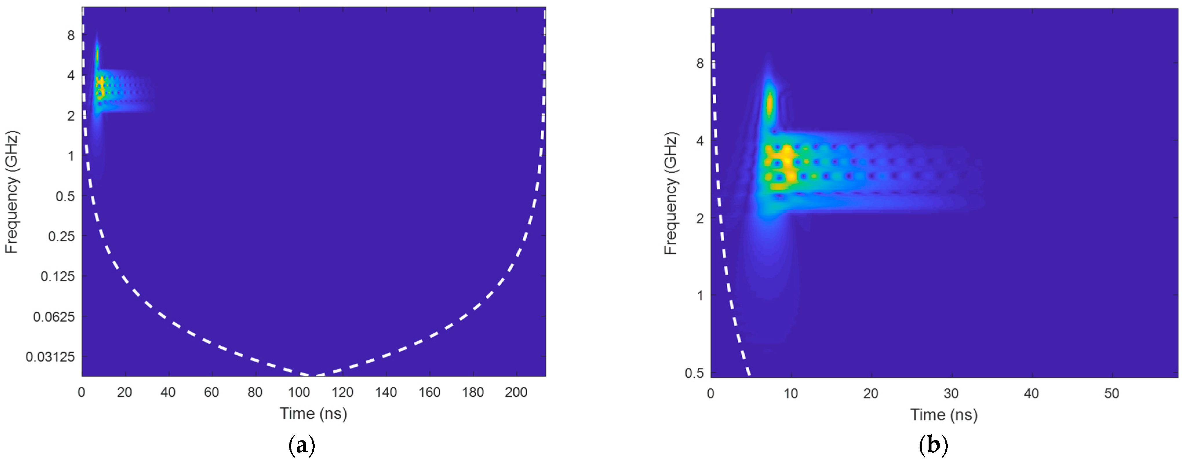
3.1. Tag Reading via CWT

Wavelet transform inherits and develops the concept of STFT, overcoming defects in window size that do not change with frequency. A wavelet that scales with frequency can analyze signals, which are used for local analysis of time and frequency [23,24]. Through wavelet basis translation and contraction, the signal is gradually refined on multiple scales. As a result, a higher time resolution is achieved in the high-frequency region and a higher-frequency resolution in the low-frequency region. With wavelet analysis, multitag scattered signals can be processed to obtain the arrival time of each tag’s scattered signal more accurately. Continuous wavelet transformation of the received signal can be written as

$$CWT\left(a,b\right)=〈r,{\psi }_{a,b}〉=\frac{1}{\sqrt{a}}\underset{-\infty }{\overset{+\infty }{\int }}r\left(t\right){\psi }^{*}\left(\frac{t-b}{a}\right)dt$$

(5)

where $\psi \left(t\right)$ is the wavelet basis; $a$ is the scaling factor and $b$ is the time shift, corresponding to frequency and time, respectively, in the time–frequency plot. We substitute (3) into (5) to obtain the following:

$$CWT\left(a,b\right)=\frac{1}{\sqrt{a}}{\int }_{-\infty }^{+\infty }p\left(t\right)\otimes tag\left(t\right)\otimes \delta \left(t-{\tau }_d\right){\psi }^{*}\left(\frac{t-b}{a}\right)dt$$

(6)

According to the Parseval theorem, the equivalent in the frequency domain is

$$CWT\left(a,b\right)=\frac{\sqrt{a}}{2\pi }{\int }_{-\infty }^{+\infty }P\left(\omega \right)Tag\left(\omega \right){\Psi }^{*}\left(a\omega \right)e^{j\omega \left({b-\tau }_d\right)}d\omega$$

(7)

where $\Psi \left(\omega \right)$ is the frequency-domain form of the wavelet basis. According to the wavelet analysis theory, the length of the wavelet basis $\psi \left(t\right)$ is finite, and the integral value is zero. When $b$ is equal to ${\tau }_d$, it peaks in the spectrum. In addition, due to a higher time resolution in the high-frequency region, it appeared to have a tapered shape in the time–frequency plot. The tag coding can be read according to the ridge distribution.

Equation (7) is extended to the multitag detection scenario, assuming ${T\mathrm{a}\mathrm{g}}_i\left(\omega \right)$ is the frequency-domain response of the $i\mathrm{t}\mathrm{h}$ tag. ${\tau }_{di}$ is the delay generated by the distance from the $i\mathrm{t}\mathrm{h}$ tag to the antenna; then, the continuous wavelet transform of the echo signal becomes the following:

$$CWT\left(a,b\right)=\frac{\sqrt{a}}{2\pi }\sum _{i=1}^N{\int }_{-\infty }^{+\infty }P\left(\omega \right){Tag}_i\left(\omega \right){\Psi }^{*}\left(a\omega \right)e^{j\omega \left({b-\tau }_{di}\right)}d\omega$$

(8)

Similarly, when $b$ equal to ${\tau }_{di}$, the tapered shape of the $i\mathrm{t}\mathrm{h}$ tag will appear in the time–frequency plot.

3.2. Time Resolution Enhancement

Although CWT has a certain time resolution, when two tags are too close, they will still interfere with each other and cannot be read correctly. Therefore, it is necessary to use an appropriate signal separation method to extract the pure scattered signal from each tag. This situation illustrates a classic “cocktail problem”, also known as the blind signal separation problem, in the field of signal processing. There are two ways of solving this kind of problem. One is to use the statistical characteristics of the signal to separate, that is, independent component analysis. The other is to use the sparse characteristics of the signal to separate. The scattered signal purification problem is more suitable for the former.

ICA application has two preconditions [25]: (1) the source signal is statistically independent, and (2) the source signal has a non-Gaussian distribution. Since the resonator-induced current generated by adjacent tags is usually weak, no significant mutual coupling phenomenon will occur; that is, the scattered signals from each tag are independent. The first condition is true. According to the quantile–quantile plot of the C-shaped tag, the normalized radar cross section constructed in the simulation part of the scattering field does not obey the Gaussian distribution, which satisfies the second condition.

A multidimensional observation matrix is needed for blind source signal separation based on ICA. Observation matrices can be constructed from multiple measurements using a single antenna or from simultaneous measurements with multiple antennas. Both methods are equivalent. Let $\mathrm{m}$ be the observation matrix dimension. Assume that there are m measuring antennas, and the scattered signal received by each antenna is a linear combination of different tag echoes. The scattered signal received by the $j\mathrm{t}\mathrm{h}$ antenna can be expressed by the following:

$$x_j\left(t\right)=a_{j1}{r}_{tag1}\left(t\right)+a_{j2}{r}_{tag2}\left(t\right)+\cdots +a_{jn}{r}_{tagn}\left(t\right)$$

(9)

Written in matrix form, this becomes

$$X=\left[\begin{array}{cccc}{a}_{11}& a_{12}& \cdots & a_{1n}\\ a_{21}& a_{22}& \cdots & a_{2n}\\ ⋮& ⋮& \ddots & ⋮\\ a_{m1}& a_{m2}& \cdots & a_{mn}\end{array}\right]\left[\begin{array}{c}{r}_{tag1}\left(t\right)\\ r_{tag2}\left(t\right)\\ \begin{array}{c}⋮\\ r_{tagn}\left(t\right)\end{array}\end{array}\right]=AR$$

(10)

in which

$$A=\left[\begin{array}{cccc}{a}_{11}& a_{12}& \cdots & a_{1n}\\ a_{21}& a_{22}& \cdots & a_{2n}\\ ⋮& ⋮& \ddots & ⋮\\ a_{m1}& a_{m2}& \cdots & a_{mn}\end{array}\right],R=\left[\begin{array}{c}{r}_{tag1}\left(t\right)\\ r_{tag2}\left(t\right)\\ \begin{array}{c}⋮\\ r_{tagn}\left(t\right)\end{array}\end{array}\right]$$

(11)

The unmixed matrix $B$ is obtained via ICA, and the pure tag scattered signal is

$$\widehat{R}=BAR$$

(12)

Finally, the tag code is read.

According to the central limit theorem, mixed independent random variables tend to have Gaussian distributions. Therefore, the independence of $\widehat{R}$ can be measured by its non-Gaussianity. The goal of ICA is to find an unmixed matrix $W$ such that $\widehat{R}$ has the strongest non-Gaussianity [26]. In ICA, kurtosis or negentropy, two higher-order statistics, are usually chosen to measure non-Gaussianity. The greatest advantage of using kurtosis as the objective function is that it is simple to calculate, and there are no false local extreme points in infinite cyclic sampling [27,28]. However, for independent components that obey a hyper-Gaussian distribution, using kurtosis as the objective function does not meet the requirement of minimizing asymptotic variance. In addition, kurtosis may be extremely sensitive to outliers, and its value may only depend on a small number of marginal observations, which may be wrong or irrelevant to the problem [29]. As a non-Gaussian measure, negentropy is relatively stable and has a strict statistical theoretical background.

The fast fixed-point ICA (FastICA) based on negentropy adopts the Newton iterative process, which has a good convergence effect and guaranteed convergence speed. Moreover, this iterative process does not need to adjust the step size [30]. The FastICA algorithm is as follows. Before executing the ICA computation, Equation (12) is whitened for preprocessing and rewritten as

$$Y=B^{T}Z$$

(13)

in which $B=\left[\begin{array}{ccc}{b}_1& b_2& \begin{array}{cc}\dots & b_n\end{array}\end{array}\right]$ is the unmixed matrix and $Z$ is the deaveraged and whitened observation data get from $X$ in (10); that is, each independent scattered signal estimation can be expressed as follows:

$$y_i=b_i^{T}Z$$

(14)

The $y_i$ distribution function $p\left(y_i\right)$ is similar to the standard normal distribution $p_g\left(y_i\right)$ and can be approximated as a weighted sum of multiple non-polynomial functions $F^{\left(i\right)}\left(·\right)$.

$$p\left(y_i\right)=p_g\left(y_i\right)\left(1+\sum _{i=1}^M{F}^{\left(i\right)}\left(y_i\right)\right)$$

(15)

FastICA algorithm solves the $b_i$ iterative formula as follows:

$$\left\{\begin{array}{c}{b}_i\left(k+1\right)=E\left\{Zf\left(b_i^T\left(k\right)Z\right)\right\}-E\left\{f^{’}\left(b_i^T\left(k\right)\right)\right\}{b}_i\left(k\right)\\ b_i\left(k+1\right)=\frac{b_i\left(k+1\right)}{‖b_i\left(k+1\right)‖}\end{array}\right.$$

(16)

where $f\left(·\right)$ is the derivative of $F\left(·\right)$ in (15). The common functions for $F\left(·\right)$ and $f\left(·\right)$ are shown in

Table 1. Common functions for $f\left(·\right)$.

$$\mathit{F}\left(\mathit{y}\right)$$	$$\mathit{f}\left(\mathit{y}\right)$$	$${\mathit{f}}^{\mathbf{\prime }}\left(\mathit{y}\right)$$
$\frac{1}{a}logcosh\left(ay\right)$	$tanh\left(ay\right)$	$a\left[1-{tanh}^2\left(ay\right)\right]$
${-e}^{-\frac{y^2}{2}}$	${ye}^{-\frac{y^2}{2}}$	${\left(1-y^2\right)e}^{-\frac{y^2}{2}}$
$y^4$	${4y}^3$	${12y}^2$

. By substituting (14) into (5), the time–frequency plot of the $ith$ tag can be obtained.

$${CWT}_{tagi}\left(a,b\right)\frac{1}{\sqrt{a}}\underset{-\infty }{\overset{+\infty }{\int }}{b}_i^{T}Z·{\psi }^{*}\left(\frac{t-b}{a}\right)dt$$

(17)

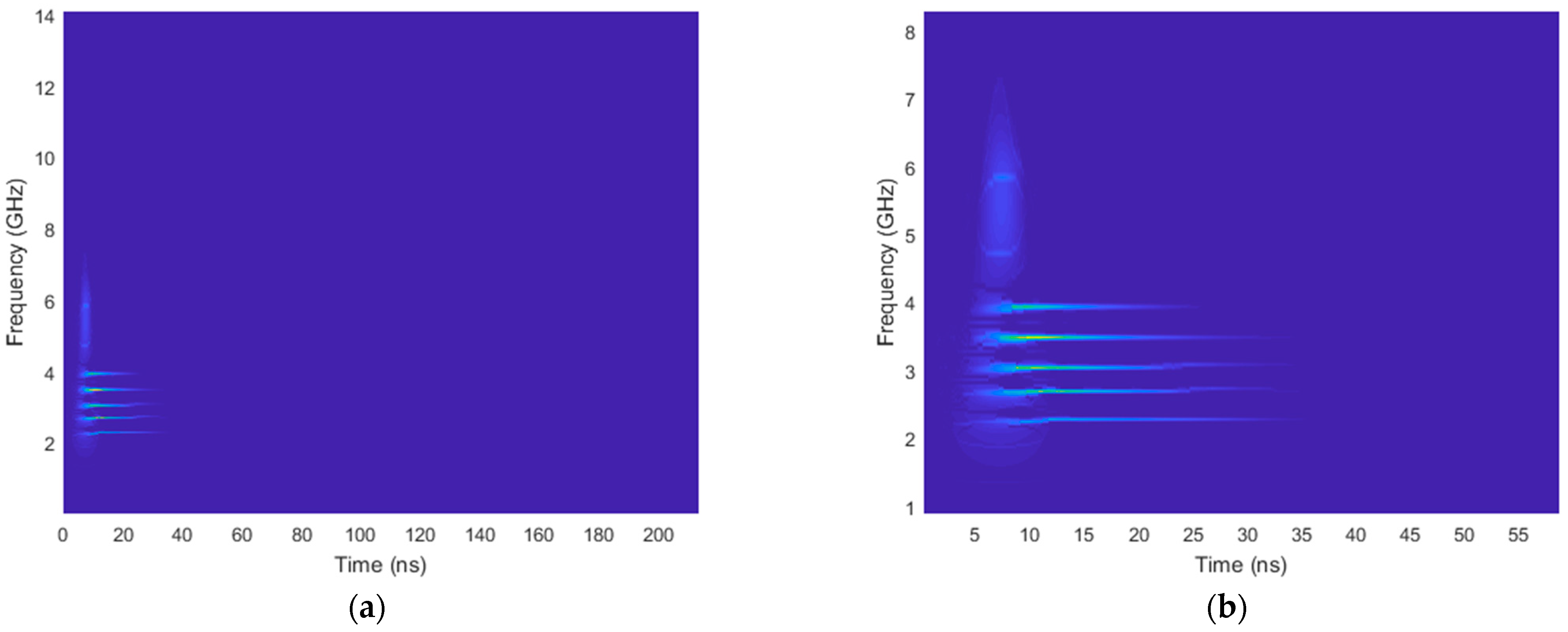
3.3. Frequency Focusing

CWT has high time resolution in a high-frequency region and high frequency resolution in a low-frequency region. However, from another perspective, the time–frequency plot cannot present high time and frequency resolution at the same time, leading to low resolution and poor readability. To achieve a clearer time–frequency plot, a wavelet synchrosqueezed transform (WSST) was used to redistribute the energy in the scale direction to the frequency direction, thereby enhancing the energy concentration [31].

In the SST, the concept of phase transformation is introduced [32]. The instantaneous frequency of the tag scatter signal is denoted as

$$\left\{\begin{array}{c}\omega \left(a,b\right)=\frac{1}{j2\pi }\frac{\partial }{\partial b}\mathit{log}\left|CWT\left(a,b\right)\right|=\frac{\frac{\partial }{\partial b}CWT\left(a,b\right)}{j2\pi CWT\left(a,b\right)}\\ CWT\left(a,b\right)\ne 0\end{array}\right.$$

(18)

In the time–frequency plot, the WSST is represented by $\mathrm{W}\mathrm{S}\mathrm{S}\mathrm{T}\left(\mathsf{\xi },\mathrm{b}\right)$, which is defined as

$$WSST\left(\xi ,b\right)={\int }_{\left\{a\in {\mathbb{R}}_{+}: CWT\left(a,b\right)\ne 0\right\}}CWT\left(a,b\right)\delta \left(\omega \left(a,b\right)-\xi \right)\frac{da}{a}$$

(19)

3.4. Flowchart

A flowchart of this innovative method based on wavelet analysis is shown in Figure 2. Firstly, the scatter signal is implemented via CWT, and the number of tags is identified from the high-frequency region of the time–frequency plot. When there are multiple tags in the reading zone and obvious interference in the time–frequency plot, the observation dataset for ICA is constructed from multiple measurements. Multiple measurements can be achieved by using multiple readers, changing the antenna direction, or moving the antenna position. Then, the dataset is centralized and whitened. The scattered signal of each tag is separated via ICA. Finally, WSST is performed on each pure scatter signal, reading the code from the time–frequency plot.

When multiple tags are at the same distance from the antenna, the number of tags cannot be accurately identified from the CWT time–frequency plot. In practice, multiple antennas can be deployed to read. However, due to geometric relations, tags cannot be at the same distance from each antenna. Therefore, to simplify the problem, a single antenna is used to read tags with different distances for simulation verification. Another potential failure scenario occurs when some tag scattered signals are too weak and become overwhelmed by other scattered signals, making it impossible to determine the number of tags. In ICA, these problems can be classified as problems of determining the number of independent components. There is a significant amount of research [33,34] on this subject, which will not be detailed here.

4. Simulation

During the simulation, C-shaped chipless RFID tags [35] are modeled and constructed in FEKO software with version 2017-293043 (x64) to obtain tag scattering echo data. Then, the proposed method is used in MatLab to process the data and verify the accuracy. The correctness of the proposed method was verified using single-tag readings, multitag readings, and noise conditions.

4.1. Parameter Selection Strategy

In wavelet analysis, wavelet basis selection plays a key role in transformation performance. At present, wavelet selection is carried out in a heuristic manner or using an empirical trial-and-error approach [36].

The wavelet basis function has five important properties: orthogonality, symmetry, regularity, vanishing moment, and compact support [37]. Orthogonality, symmetry, and regularity mainly affect wavelet signal recovery performance. Since the proposed method only reads codes in the time–frequency plot, these three properties were not considered. The compact support (support width) reflects the wavelet functions’ localization ability. The smaller the support width, the stronger the localization ability of wavelet basis functions, and the lower the computational complexity of wavelet packet transformation. The vanishing moment determines the rate of convergence when the wavelet approximates a smooth function. It shows the degree of energy concentration after wavelet transformation [38]. Compact support and vanishing moments are the key parameters of the proposed method.

Most common wavelets used with CWT for analyzing nonstationary data are Morlet, Morse, and bump wavelets [39]. The Morlet wavelet function expression is

$${\Psi }_{morlet}\left(t\right)={\pi }^{-\frac{1}{4}}{e}^{i{\omega }_{0}t}{e}^{-\frac{t^2}{2}}$$

(20)

where ${\mathsf{\omega }}_0$ is a frequency parameter that controls the frequency of the wavelet function; $i$ is the imaginary unit. ${\pi }^{-\frac{1}{4}}$ is used to normalize the amplitude of the wavelet function to ensure that the wavelet function’s energy remains consistent at different scales. Similar to STFT, this expression is the product of a complex exponential function and a Gaussian function. Therefore, the Morlet wavelet was not used.

The Fourier transform of the generalized Morse wavelet is

$${\Psi }_{morse}\left(\omega \right)=U\left(\omega \right)a_{p,\gamma }{\omega }^{\frac{P^2}{\gamma }}{e}^{{-\omega }^{\gamma }}$$

(21)

where $U\left(\omega \right)$ is the unit step; $a_{p,\gamma }$ is a normalizing constant; $P^2$ is the time-bandwidth product; and $\mathsf{\gamma }$ characterizes the symmetry of the Morse wavelet. Much of the literature about Morse wavelets uses $\beta$, which can be considered a decay or compactness parameter, rather than the time-bandwidth product, $P^2=\beta \gamma$. As the $\beta$ value increases, the frequency localization improves while time localization worsens, and vice versa. Due to the above reasons, an appropriate $\beta$ value must be selected, which is tested in Section 4.2.

The bump wavelet frequency-domain expression is as follows:

$${\Psi }_{bump}\left(\omega \right)=e^{1-\frac{1}{1-\frac{{\left(\omega -u\right)}^2}{{\sigma }^2}}} , u-\sigma <\omega <u+\sigma$$

(22)

The $\sigma$ values range from 0.1 to 1.2, and the $u$ range is $\left[\mathrm{3,6}\right]$. The smaller the $\sigma$ value, the narrower the ${\mathsf{\Psi }}_{bump}\left(\omega \right)$ shape and the higher the frequency resolution obtained. In the proposed method, a smaller $\sigma$ value should be selected for the bump wavelet.

4.2. Signal Tag Reading

Figure 3 shows a C-shaped chipless tag with a 5-bit coding capacity created in FEKO 2017 software.

Figure 3a shows the physical structure of the tag, which measures 30 × 22 × 0.8 mm³. The green part is an insulating substrate with the dielectric mass constant set to 4.6 to simulate FR4 material. The yellow part is a perfect electrical conductor. The corresponding RCS is shown in Figure 3b. It was calculated using domain Green’s function method in FEKO software. There are five resonances at 2.3 GHz, 2.7 GHz, 3.0 GHz, 3.5 GHz, and 3.9 GHz. For frequency-domain chipless RFID tags, the resonance at specified frequencies represents logic 1, and no resonance represents logic 0; therefore, the tag code is “11111”. The all-1 coding tag was used to verify whether the time–frequency plot obtained via wavelet analysis had a sufficient frequency resolution to correctly identify all resonant frequency points. Based on the RCS, scattered signals can be obtained using Gaussian pulses as excitation signals. Then, MatLab software was used to perform CWT of the scattered signal according to (6). The time–frequency distribution of the scatter signal was calculated from Morse and bump wavelets. For the bump wavelet, Figure 4 presents the time–frequency plot when $\sigma =0.3$ and $u=5$. Five color bands in the coding frequency range correspond to the five resonators on the tag. However, no matter how the $\mathsf{\gamma }$ and $\beta$ values of the Morse wavelet are adjusted, a time–frequency plot with good recognition cannot be obtained as shown in Figure 5. The reason for this is that the similarity between the Morse wavelet and the excitation Gaussian pulse is too low. Wavelet selection based on the similarity between signals and wavelets is one of the selection criteria [40]. Accordingly, the bump wavelet was selected for simulation. WSST was used to process the tag scattered signals, and the resulting time frequency plot is shown in Figure 6.

After WSST, the energy in the scale direction becomes concentrated and the time–frequency plot is more readable. Power valleys appear above each of the five horizontal bands, hence the tag code “11111”.

4.3. Multitag Reading

Frequency chipless RFID tags use resonators to achieve binary coding. Each resonator corresponds to a resonant frequency point in the echo. Resonance at a particular frequency is defined as 1; otherwise, it is 0. To verify the multitag anti-collision capabilities of the proposed method, two tags coded as “01010” and “10101” were selected to read and test whether the five resonant frequency points would be correctly assigned to the corresponding tag. Two C-shaped tag models with dimensions of 30 × 22 × 0.8 mm³ were constructed in FEKO software. The simulation scenario and the tag structures are shown in Figure 7.

The antenna received the tag scattered signal at a distance of 1 m from the tag. The smaller the distance between two tags, the more serious the tag echo interference is. To verify the multitag detection capabilities of the proposed method, the spacing d was set to 0.45 m, 0.2 m, and 0.05 m, respectively. The dataset consisted of two measurements in which the antenna pointed in different directions. The mixed echo obtained via each measurement was a linear combination of two tag scattered signals as (9). The WSST time–frequency plots of mixed scatter signals are shown in Figure 8.

When the distance between the two tags was 0.2 m, they gradually merged in the time–frequency plot. When the distance between the tags was 0.05 m, the frequency band of the two tags completely overlapped, and the number of tags could not be identified. Figure 9 shows the WSST results after ICA was adopted to achieve signal separation.

As seen in Figure 8, the tag code can be read successfully. Although pale interfering fringes appear in the time–frequency plot as the spacing decreases, they do not affect the correct reading.

5. Performance Comparison

5.1. Complexity

WSST is based on CWT and uses a synchrosqueezed transform to reassign the time–frequency plot. SST is also applicable to time–frequency plots generated via STFT. ICA’s source separation algorithm also applies to STMPM, STFT, and CWT. Therefore, the complexity of STMPM, STFT, and CWT became the comparison object.

According to (5), $N$ rounds of multiplication and addition operations are required to compute a point $CWT\left(a_0,b_0\right)$ in the time–frequency plot, and $N$ is the number of signal points. $b$ is continuously valued within $\left[1,N\right]$, and a is valued at a fixed interval in the tag frequency band. Therefore, the time complexity of CWT is $O\left({MN}^2\right)$, where $M$ is the dimension of the scale vector. The spectrum calculation of the STFT at time $t$ is shown in (20):

$$STFT\left(t,\omega \right)={\int }_{-\infty }^{+\infty }x\left(\tau \right)w^{*}\left(t-\tau \right)e^{-j\omega \tau }d\tau$$

(23)

where $x\left(t\right)$ is the scatter signal; the length is $N$; and $w\left(t\right)$ is the window function with a width of $M$. To complete STFT, it is necessary to multiply and add $N\times M$ times with a corresponding time complexity of $O\left(MN\right)$. The core of STMPM is matrix singular value decomposition (SVD). The complexity of SVD is $O\left({LM}^2\right)$, where $M$ is the number of columns in the Hankel matrix, corresponding to the width of the time window in STMPM. $L$ is the number of rows in the Hankel matrix, generally taking values between $M/3$ and $M/2$. For a signal of length $N$, the time window slides from start to end with a corresponding computational complexity of $O\left({LM}^{2}N\right)$. The complexity and average running time are shown in

Table 2. STMPM, STFT, and CWT running time comparison.

Algorithm Type	Time Complexity	Run Time (seconds)
STMPM	$O\left(L{M}^{2}N\right)$	9.351043
STFT	$O\left(MN\right)$	0.075236
CWT	$O\left(M{N}^2\right)$	0.220115

.

The test platform was a DELL XPS 15 9570 computer with an I5-8300H processor and 8 GB of memory. The simulation software was MATLAB R2019a. In the test, the signal sampling frequency was 28 GHz and the sampling number was 6004. The STFT window width was 256 points and the Fourier transform points value was 512. The STMPM window width was 113 points. CWT calculated the wavelet coefficients at 384 scales. The STMPM, STFT, and CWT algorithms were used to process the tag scattered signal encoded as “11111”. The results are shown in Figure 10.

Three methods correctly identified five resonance frequency points. Among STMPM, STFT, and CWT, STFT had the shortest operation time. Compared to STMPM, CWT’s processing time was significantly reduced from 9.35 s to 0.22 s, indicating a significant improvement.

5.2. Range Resolution

To compare the range resolution of the proposed method with those of STMPM and STFT, these methods were used to read the tag code in the Figure 7 simulation scenario. Figure 11 shows the results for when the distance between the two tags was 0.2 m.

STMPM and STFT are sensitive to the window width. When the window width is reduced, the time resolution can be improved at the expense of the frequency resolution. STMPM determines the tag scattering opening time based on the pole distribution stability and thus determines the tag number. According to the test results, the STMPM failed to recognize the number of tags at a space of 0.2 m. When the window width of STFT was 2.25 ns, the tag number was identifiable; however, in practical application, it is necessary to find a way to determine the appropriate window width. It is difficult to find a balance between the frequency resolution and time resolution for the STFT method. The test results with a tag spacing of 0.05 m are shown in Figure 12.

Since CWT has a higher time resolution in the high-frequency region, the tag number can be identified from high-frequency details in the time–frequency plot. By contrast, STFT cannot distinguish between two tags and read codes. When the STFT window width was further reduced to 0.55 ns, the time–frequency plot was vertically striped, and the tag number could not be identified.

5.3. Robustness

To better simulate real environments, the proposed algorithm’s detection ability was verified under different SNR conditions. The tags used were the same as those described in Section 4.2 and Section 4.3. The spacing was set to 0.45 m to ensure that all three algorithms could be read correctly under noise-free conditions. Gaussian white noise was added to the mixed echo, and the signal tag reading simulation results under different signal-to-noise ratio conditions are shown in Figure 13.

It can be seen from Figure 13 that STMPM is the most sensitive to noise and can no longer work in the 0 dB SNR condition. By contrast, STFT and WSST perform better. When the SNR is reduced to −10 dB, WSST and STFT are barely recognizable. Artificial intelligence may yield better results. Figure 14, Figure 15 and Figure 16 show multittag recognition simulation results under noisy conditions.

As shown in Figure 14, the proposed algorithm is greatly affected by Gaussian noise in multitag detection. It is also effective when the SNR is greater than or equal to 20 dB. Under noise conditions in Figure 15 and Figure 16, there is no significant difference between multitag detection and single-tag detection for STFT and STMPM. The reason for this is that ICA requires a non-Gaussian signal distribution, and Gaussian white noise in the echo signal reduces the separation effect.

Three points can be drawn from the above comparison: (1) Compared to STMPM, CWT requires significantly less computation, and the tag pole number is not required. Regarding range resolution, CWT has obvious advantages. (2) Compared to STFT, CWT avoids window width selection and uses a high temporal resolution in the high-frequency region to identify the number of tags, and a high-frequency resolution in the low-frequency region to read the tag code. (3) Due to ICA’s non-Gaussian requirements, the proposed method needs better scattering signal quality. Tag readings will be seriously affected if the Gaussian white noise interference is significant.

Table 3. STMPM, STFT, proposed method comparison.

Algorithm Type	STMPM	STFT	Proposed Method
Code Reading	Time pole plot Poles distribution	Time–frequency plot Energy distribution	Time–frequency plot Energy distribution
Key Parameter	Poles number Search step size window width	Search step size window width	Wavelet function
Computational Efficiency	STMPM for every time window	FT for every time window	CWT+WSST for whole signal
Minimum Tag Spacing	≥0.2 m	≥0.05 m	0.05 m
Robustness	SNR ≥ 10 dBm	SNR ≥ 0 dBm	SNR ≥ 20 dBm

compares the three methods.

6. Conclusions

In this paper, wavelet analysis was used to read chipless RFID tags, and a CWT+ICA+WSST multitag detection method was proposed. C-shaped chipless RFID tag models with 5-bit coding capacities were constructed in FEKO software, and the scattering signals were obtained by solving the model with domain Green’s function method. When the SNR was greater than 20 dB, the mixed echo signal was processed via the proposed method. Two tags with a spacing of 0.05 m were also read correctly. This novel method improves multitag detection ability while reducing the amount of computation compared to STMPM. The selection of the window width parameter was avoided. In other words, this method can be used to reduce the cost and size of the reader based on reading performance. The proposed method will be further verified in actual environments.

The proposed method can be used for chipless RFID tag detection in a pipeline. Several antennas were installed on both sides of a production line to receive scattered signals, and ICA and WSST were applied to the computing unit to extract the ridge of time–frequency plots and read codes. Appropriate wavelet functions should be selected for analysis according to different excitation signals and chipless RFID tag types in practical applications. In theory, wavelet analysis can be used simultaneously with signal processing techniques such as MIMO and TRM. Array antenna signal processing technologies are used for beamforming. When there are multiple tags in the main lobe, the proposed method can read codes. Additionally, artificial intelligence can be used for time–frequency plot analysis.

References

1. Preradovic, S.; Karmakar, N.C. Design of fully printable planar chipless RFID transponder with 35-bit data capacity. In Proceedings of the 2009 European Microwave Conference (EuMC), Rome, Italy, 29 September–1 October 2009; pp. 13–16. [Google Scholar]
2. Islam, M.A.; Karmakar, C.N. A novel compact printable dualpolarized chipless RFID system. IEEE Trans. Microw. Theory Tech. 2012, 60, 2142–2151. [Google Scholar] [CrossRef]
3. Zhao, F.; Zou, C.; Xu, L.; He, Y. Design of a printable chipless RFID tag based on multi-resonator. Chin. Comm. Netw. 2018, 44, 113–116. [Google Scholar]
4. Analogictips. Available online: https://www.analogictips.com/how-chipless-rfids-will-revolutionize-consumer-and-defense-applications/ (accessed on 12 April 2024).
5. Herrojo, C.; Paredes, F.; Mata-Contreras, J.; Martín, F. Chipless-RFID: A Review and Recent Developments. Sensors 2019, 19, 3385. [Google Scholar] [CrossRef]
6. El-Hadidy, M.; El-Awamry, A.; Fawky, A.; Khaliel, M.; Kaiser, T. A novel collision avoidance MAC protocol for multi-tag UWB chipless RFID systems based on Notch Position Modulation. In Proceedings of the 2015 9th European Conference on Antennas and Propagation (EuCAP), Lisbon, Portugal, 13–17 April 2015; pp. 1–5. [Google Scholar]
7. Xia, Z. Research on Chipless Multitag MAC Protocol. Master’s Thesis, Southwest University of Science and Technology, Mianyang, China, 22 May 2019. (In Chinese). [Google Scholar]
8. Su, C.; Zou, C.; Jiao, L.; Zhang, Q. A MIMO Radar Signal Processing Algorithm for Identifying Chipless RFID Tags. Sensors 2021, 21, 8314. [Google Scholar] [CrossRef] [PubMed]
9. Su, C.; Zou, C.; Jiao, L. Chipless RFID identification based on time reversal algorithm. J. Electromagn. Waves Appl. 2023, 37, 1045–1065. [Google Scholar] [CrossRef]
10. Costa, F.; Borgese, M.; Gentile, A.; Buoncristiani, L.; Genovesi, S.; Dicandia, F.A.; Bianchi, D.; Monorchio, A.; Manara, G. Robust Reading Approach for Moving Chipless RFID Tags by Using ISAR Processing. IEEE Trans. Microw. Theory Tech. 2018, 66, 2442–2451. [Google Scholar] [CrossRef]
11. Rezaiesarlak, R.; Manteghi, M. A new anti-collision algorithm for identifying chipless RFID tags. In Proceedings of the 2013 IEEE Antennas and Propagation Society International Symposium (APSURSI), Orlando, FL, USA, 7–13 July 2013; pp. 1722–1723. [Google Scholar]
12. Rezaiesarlak, R.; Manteghi, M. Accurate extraction of early-late time responses using short-time matrix pencil method for transientanalysis of scatterers. IEEE Trans. Antennas Propag. 2015, 63, 4995–5002. [Google Scholar] [CrossRef]
13. Ali, Z.; Perret, E.; Barbot, N.; Siragusa, R. Extraction of Aspect-Independent Parameters Using Spectrogram Method for Chipless Frequency-Coded RFID. IEEE Sens. J. 2021, 21, 6530–6542. [Google Scholar] [CrossRef]
14. Vena, A.; Perret, E.; Tedjini, S. A fully printable Chipless RFID tag with detuning correction technique. IEEE Microw. Wirel. Compon. Lett. 2012, 22, 209–211. [Google Scholar] [CrossRef]
15. Karmakar, N.C.; Amin, E.M.; Saha, J.K. Chipless RFID Reader Architecture. In Chipless RFID Sensors, 1st ed.; Wiley: New York, NY, USA, 2016; pp. 217–224. [Google Scholar] [CrossRef]
16. Preradovic, S.; Karmakar, N.C. Multiresonator based chipless RFID tag and dedicated RFID reader. In Proceedings of the 2010 IEEE MTT-S International Microwave Symposium, Anaheim, CA, USA, 23–28 May 2010; pp. 1520–1523. [Google Scholar]
17. Koswatta, R.V.; Karmakar, N.C. A novel reader architecture based on UWB chirp signal interrogation for multiresonator-based chipless RFID tag reading. IEEE Trans. Microw. Theory Tech. 2012, 60, 2925–2933. [Google Scholar] [CrossRef]
18. Forouzandeh, M.; Karmakar, N. Self-Interference Cancelation in Frequency-Domain Chipless RFID Readers. IEEE Trans. Microw. Theory Tech. 2019, 67, 1994–2009. [Google Scholar] [CrossRef]
19. Forouzandeh, M.; Karmakar, N. Towards the Improvement of Frequency-domain Chipless RFID Readers. In Proceedings of the 2018 IEEE Wireless Power Transfer Conference (WPTC), Montreal, QC, Canada, 3–7 June 2018; pp. 1–4. [Google Scholar]
20. Rezaiesarlak, R.; Manteghi, M. Short-Time Matrix Pencil Method for Chipless RFID Detection Applications. IEEE Trans. Antennas Propag. 2014, 61, 2801–2806. [Google Scholar] [CrossRef]
21. Rezaiesarlak, R.; Manteghi, M. A Space–Time–Frequency Anticollision Algorithm for Identifying Chipless RFID Tags. IEEE Trans. Antennas Propag. 2014, 62, 1425–1432. [Google Scholar] [CrossRef]
22. Karmakar, N.; Amin, E. Short Time Fourier Transform (STFT) for collision detection in chipless RFID systems. In Proceedings of the 2015 International Symposium on Antennas and Propagation (ISAP), Hobart, TAS, Australia, 9–12 November 2015; pp. 1–4. [Google Scholar]
23. Rioul, O.; Vetterli, M. Wavelets and signal processing. IEEE Signal Proc. Mag. 1991, 8, 14–38. [Google Scholar] [CrossRef]
24. Daubechies, I. The wavelet transform, time-frequency localization and signal analysis. IEEE Trans. Inf. Theory 1990, 36, 961–1005. [Google Scholar] [CrossRef]
25. Hyvärinen, A.; Karhunen, J.; Oja, E. What is Independent Component Analysis? In Independent Component Analysis, 1st ed.; Wiley: New York, NY, USA, 2001; pp. 151–154. [Google Scholar]
26. Hyvärinen, A.; Karhunen, J.; Oja, E. ICA by Maximization of Nongaussianity. In Independent Component Analysis, 1st ed.; Wiley: New York, NY, USA, 2001; pp. 165–201. [Google Scholar]
27. Hyvärinen, A.; Oja, E. A Fast Fixed-Point Algorithm for Independent Component Analysis. Neural Comput. 1997, 9, 1483–1492. [Google Scholar] [CrossRef]
28. Zarzoso, V.; Comon, P. Robust Independent Component Analysis by Iterative Maximization of the Kurtosis Contrast with Algebraic Optimal Step Size. IEEE Trans. Neural Netw. 2010, 21, 248–261. [Google Scholar] [CrossRef] [PubMed]
29. Hyvärinen, A. One-unit contrast functions for independent component analysis: A statistical analysis. In Proceedings of the Neural Networks for Signal Processing VII—1997 IEEE Signal Processing Society Workshop, Amelia Island, FL, USA, 24–26 September 1997; pp. 388–397. [Google Scholar]
30. Hyvärinen, A. Fast and robust fixed-point algorithms for independent component analysis. IEEE Trans. Neural Netw. 1999, 10, 626–634. [Google Scholar] [CrossRef]
31. Meignen, S.; Oberlin, T.; McLaughlin, S. A New Algorithm for Multicomponent Signals Analysis Based on SynchroSqueezing: With an Application to Signal Sampling and Denoising. IEEE Trans. Signal Process. 2012, 60, 5787–5798. [Google Scholar] [CrossRef]
32. Daubechies, I.; Lu, J.; Wu, H.-T. Synchrosqueezed Wavelet Transforms: An empirical mode decomposition-like tool. Appl. Comput. Harmon. Anal. 2011, 30, 243–261. [Google Scholar] [CrossRef]
33. Kairov, U.; Cantini, L.; Greco, A.; Molkenov, A.; Czerwinska, U.; Barillot, E.; Zinovyev, A. Determining the optimal number of independent components for reproducible transcriptomic data analysis. BMC Genom. 2017, 18, 712. [Google Scholar] [CrossRef] [PubMed]
34. Mur, A.; Dormido, R.; Duro, N.; Mercader, D. An unsupervised method to determine the optimal number of independent components. Expert Syst. Appl. 2017, 75, 56–62. [Google Scholar] [CrossRef]
35. Mumtaz, M.; Amber, S.F.; Ejaz, A.; Habib, A.; Jafri, S.I.; Amin, Y. Design and analysis of C shaped chipless RFID tag. In Proceedings of the 2017 International Symposium on Wireless Systems and Networks (ISWSN), Lahore, Pakistan, 19–22 November 2017; pp. 1–5. [Google Scholar]
36. Sahoo, G.R.; Freed, J.H.; Srivastava, M. Optimal Wavelet Selection for Signal Denoising. IEEE Access 2024, 12, 45369–45380. [Google Scholar] [CrossRef]
37. Cheng, L.; Li, D.; Li, X.; Yu, S. The Optimal Wavelet Basis Function Selection in Feature Extraction of Motor Imagery Electroencephalogram Based on Wavelet Packet Transformation. IEEE Access 2019, 7, 174465–174481. [Google Scholar] [CrossRef]
38. Peng, Z.; Wang, G. Study on Optimal Selection of Wavelet Vanishing Moments for ECG Denoising. Sci. Rep. 2017, 7, 4564. [Google Scholar] [CrossRef]
39. Silik, A.; Noori, M.; Altabey, W.A.; Ghiasi, R.; Wu, Z. Analytic Wavelet Selection for Time–Frequency Analysis of Big Data Form Civil Structure Monitoring. In Proceedings of the 10th International Conference on Structural Health Monitoring of Intelligent Infrastructure (SHMII 10), Porto, Portugal, 30 June–2 July 2021. [Google Scholar]
40. Ngui, W.K.; Leong, M.S.; Hee, L.M.; Abdelrhman, A.M. Wavelet Analysis: Mother Wavelet Selection Methods. Appl. Mech. Mater. 2013, 393, 953–958. [Google Scholar] [CrossRef]
Figure 1. Frequency-domain coded chipless RFID system.
Electronics 13 02375 g001
Figure 2. Multitag detection flowchart.
Electronics 13 02375 g002
Figure 3. Frequency-domain code chipless RFID tag: (a) tag structure; and (b) tag RCS.
Electronics 13 02375 g003
Figure 4. CWT time–frequency plot of single-tag scattered signals using bump wavelets: (a) overall plot (bump), and (b) detailed plot (bump).
Electronics 13 02375 g004
Figure 5. CWT time–frequency plot of single-tag scattered signals using Morse wavelets: (a) γ = 3 , β = 10 ; (b) γ = 3 , β = 40 ; (c) γ = 1.5 , β = 10 ; and (d) γ = 1.5 , β = 40 .
Electronics 13 02375 g005
Figure 6. WSST time–frequency plot of single-tag scattered signals: (a) overall plot, and (b) detailed plot.
Electronics 13 02375 g006
Figure 7. Multitag simulation configuration: (a) simulation scenario; (b) tag1 structure; and (c) tag2 structure.
Electronics 13 02375 g007
Figure 8. Multitag simulation configuration: (a) d = 0.45 m; (b) d = 0.2 m; and (c) d = 0.05 m.
Electronics 13 02375 g008
Figure 9. WSST time–frequency plot after ICA separation: (a) Tag1 result, d = 0.45 m; (b) Tag2 result, d = 0.45 m; (c) Tag1 result, d = 0.2 m; (d) Tag2 result, d = 0.2 m; (e) Tag1 result, d = 0.05 m; and (f) Tag2 result, d = 0.05 m.
Electronics 13 02375 g009
Figure 10. Single-tag read, tag id = “11111”: (a) STMPM pole figures; (b) STFT time–frequency plot; and (c) CWT time–frequency plot.
Electronics 13 02375 g010
Figure 11. Resolution test, d = 0.2 m: (a) STMPM, window width = 4 ns; (b) STMPM, window width = 2 ns; (c) STMPM, window width = 1 ns; (d) STFT, window width = 9 ns; (e) STFT window width = 4.5 ns; (f) STFT, window width = 2.25 ns; (g) CWT; and (h) WSST.
Electronics 13 02375 g011
Figure 12. Resolution test, d = 0.05 m: (a) CWT overall plot; (b) CWT, high-frequency detail; (c) STFT, windows with = 2.25 ns; (d) STFT, windows with = 1.1 ns; and (e) STFT, windows with = 0.55 ns.
Electronics 13 02375 g012
Figure 13. Signal tag reading robustness test: (a) WSST, SNR = 0 dB; (b) STFT, SNR = 0 dB, windows with = 4.5 ns; (c) STMPM, SNR = −0 dB, windows with = 4 ns; (d) WSST, SNR = −10 dB; (e) STFT, SNR = −10 dB, windows with = 4.5 ns; and (f) STMPM, SNR = −10 dB, windows with = 4 ns.
Electronics 13 02375 g013
Figure 14. Multitag reading robustness simulation results of the proposed method (d = 0.05 m): (a) CWT, SNR = 20 dB; (b) Tag1 result, WSST, SNR = 20 dB; (c) Tag2 result, WSST, SNR = 20 dB; (d) CWT, SNR = 10 dB; (e) Tag1 result, WSST, SNR = 10 dB; and (f) Tag2 result, WSST, SNR = 10 dB.
Electronics 13 02375 g014
Figure 15. Multitag reading robustness simulation results of STMPM (d = 0.45 m, window width = 4 ns): (a) SNR = 10 dB; (b) SNR = 0 dB; and (c) SNR = −10 dB.
Electronics 13 02375 g015
Figure 16. STFT’s multitag reading robustness simulation results (d = 0.45 m, window width = 4.5 ns): (a) SNR = 10 dB; (b) SNR = 0 dB; and (c) SNR = −10 dB.
Electronics 13 02375 g016