Abstract
Adversarial attacks have received much attention as communication network applications rise in popularity. Connected and Automated Vehicles (CAVs) must be protected against adversarial attacks to ensure passenger and vehicle safety on the road. Nevertheless, CAVs are susceptible to several types of attacks, such as those that target intra- and inter-vehicle networks. These harmful attacks not only cause user privacy and confidentiality to be lost, but they also have more grave repercussions, such as physical harm and death. It is critical to precisely and quickly identify adversarial attacks to protect CAVs. This research proposes (1) a new dataset comprising three adversarial attacks in the CAV network traffic and normal traffic, (2) a two-phased adversarial attack detection technique named TAAD-CAV, where in the first phase, an ensemble voting classifier having three machine learning classifiers and one separate deep learning classifier is trained, and the output is used in the next phase. In the second phase, a meta classifier (i.e., Decision Tree is used as a meta classifier) is trained on the combined predictions from the previous phase to detect adversarial attacks. We preprocess the dataset by cleaning data, removing missing values, and adjusting the Z-score normalization. Evaluation metrics such as accuracy, recall, precision, F1-score, and confusion matrix are employed to evaluate and compare the performance of the proposed model. Results reveal that TAAD-CAV achieves the highest accuracy with a value of 70% compared with individual ML and DL classifiers.
1. Introduction
Globally, the number of automobiles has increased dramatically due to population growth and urbanization. This growth was undoubtedly one of the main factors contributing to millions of collisions on the roads each year, as the elevated vehicle density on the roads made for an irregular, clogged traffic situation that made driving more difficult and dangerous. Intelligent Transportation Systems (ITSs) have been established as a smart technical solution to encourage smart mobility and improve road safety, among other reasons [1,2]. ITS offers several benefits, such as enhanced safety services, user-oriented mobility services, smart traffic management and monitoring, etc. [3]. Additionally, they depend on a networked infrastructure through communication linkages between cars, road users, and road sensors, known as infrastructure (V2I) and inter-vehicle (V2V). They may report road conditions and receive real-time status updates from each other, which helps to prevent dangerous situations and enhance traffic flow management [4].
Thus, because of these noteworthy developments in ITS technology, autonomous driving systems are becoming more dependable, transforming the world’s transportation infrastructure. They comprise a range of parts integrating AI and IoT (Internet of Things) technology to lessen reliance on human interaction [5,6]. Autonomous vehicle (AV) adoption ushers in a new age of transportation with several benefits to traffic safety and transportation effectiveness [7]. Connected and Automated Vehicles (CAVs), equipped with sensors, wireless connections, and onboard computing, can perceive, communicate, and control driving duties [8]. It is continually connected to the Internet, other cars, and computers through interfaces like Dedicated Short-Range Communications (DSRCs) and Cellular Vehicle-to-Everything (C-V2X). With the help of those features, CAVs can become somewhat automated and gather the data necessary for making decisions. They are also expected to significantly increase accessibility for individuals with disabilities and the elderly, lower environmental pollution, and improve road safety and system efficiency.
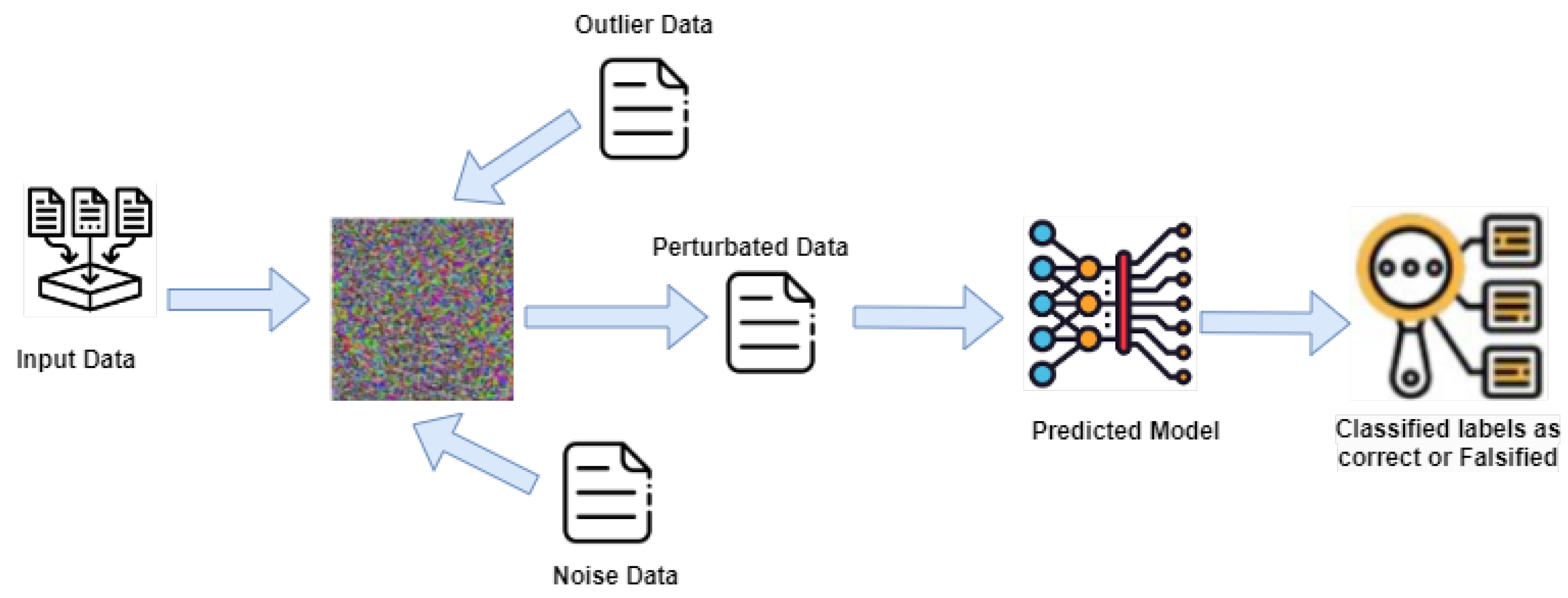
However, despite all the actions produced in this sector, some significant obstacles still prevent the widespread use of this technology. Adversarial attacks pose a significant challenge to modern machine learning models, particularly in deep learning. These attacks concern presenting carefully prepared perturbations to input data, which can lead even well-trained models to make inaccurate predictions with high confidence [9]. Figure 1 presents the working of adversarial attacks on trained models. In the context of image classification, for example, an adversarial attack might involve adding a nearly imperceptible amount of noise to an image, causing the model to misclassify it. Such attacks can be used to evaluate machine learning models’ robustness and develop defenses against them. However, they also highlight the potential vulnerabilities of these models in security-sensitive applications, such as autonomous vehicles or facial recognition systems.
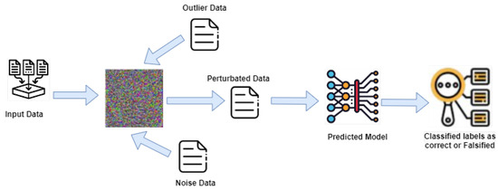
Figure 1.
Adversarial attack on trained models.
However, autonomous driving systems need a refined structure to grab those anomalies and minimize their consequences due to sensor data uncertainties generated by adversarial attacks or external elements, like weather conditions, environmental anomalies, or malfunctioning sensors. Numerous objects with distinct profiles, particularly in urban settings, the poor precision of perception sensor readings, data loss during the fusion process, and other issues can all lead to outliers [10]. These anomalies can potentially distort sensor data, resulting in inaccurate navigational judgments and incidents involving fatalities. As a result, locating and identifying these outliers in the gathered data is critical, as they might seriously harm autonomous driving systems.
1.1. Research Motivation
Researchers are still investigating numerous strategies to counteract adversarial attacks, including as input preprocessing, model hardening, and robust training procedures, to assure the dependability and safety of machine learning systems. The research has looked at several strategies to decrease the influence of these anomalies on the operation of AVs in general and autonomous cars in particular. Numerous anomaly detection and classification methods have been studied in the literature; most of these methods depend on the concept of artificial intelligence [11,12,13]. The purpose of the research was to estimate the probability that cyberattacks will cause a crash [14]. However, these methods have shortcomings. Specifically, when using deep learning techniques in CAVs, there needs to be more detection performance for both single and mixed attack types, and there needs to be a proper ensemble machine learning strategy to bolster the technique’s efficacy in identifying attacks that address limitations.
1.2. Research Contribution
To effectively detect different types of adversarial attacks in CAVs by handling the above-cited limitations, this research’s main contributions are listed below:
- Generated a novel dataset comprising three novel adversarial attacks in the CAV network traffic and normal traffic.
- Proposed a two-phased adversarial attack detection technique named TAAD-CAV, where in the first phase, an ensemble voting classifier having three machine learning classifiers and one separate deep learning classifier is trained, and the output is used in the next phase. In the second phase, a meta classifier (i.e., Decision Tree is used as a meta classifier) is trained on the combined predictions from the previous phase to detect adversarial attacks. We preprocess the dataset, such as data cleaning, removing missing values, and Z-score normalization.
- Results reveal that TAAD-CAV achieves the highest accuracy with a value of 70% compared with ML and DL classifiers.
1.3. Research Organization
This research work is further structured in multiple sections to help readers understand the study’s framework. Section 2 provides information related to previous techniques related to adversarial attacks. The proposed methodology, the dataset’s preliminaries, data preprocessing steps, and ML and DL models are all covered in detail in Section 3. The evaluation measurements, experimental results, and findings are presented in Section 4. The conclusion and future directions of the current work are also presented in this section.
2. Literature Review
The paper [15] presents a novel fuzzy decision-making model that considers several perspectives on fusion. Their methodology focuses on three steps and evaluates multi-ML classifiers for real-time adversarial attack prediction in VANETs. First, Dedicated Short-Range Communication (DSRC) data must be identified and preprocessed using conventional and fusion preprocessing techniques. Two DSRC datasets are produced due to considering two different communication scenarios: jammed and normal. Using normal preprocessing for dataset-1 and feature fusion preprocessing for dataset-2, they build multi-ML classifiers based on the DSRC datasets. At last, they assess the multi-ML classifiers using a fuzzy decision-making technique based on the fuzzy decision-making method by opinion score method (FDOSM) and an adversarial attack decision fusion matrix. The FDOSM’s External Fusion Decision (EFD) parameters choose the optimal model, give a unique rank, and handle individual ranking variation. The experiment’s findings show that the Random Forest (RF) model, used for dataset-2 using fusion preprocessing, has a score of 0.1819. In dataset-1, the K-Nearest Neighbors Algorithm (kNN) model accomplishes the highest score of 0.2048.
The article [16] presents an effective detector based on a controlled invariant subspace for detecting hidden attacks. This research is unique because it uses a real-time trajectory space generation approach and depends on the vehicle dynamics model for system state estimate. The suggested detector creates a trajectory subspace using an offline incremental-learning-based rapidly expanding random tree approach. Trajectories that deviate from this subspace are classified as anomalies. Additionally, taking into account the dynamic performance limits of the vehicle, this research offers a distance-measuring approach that integrates a radial basis function neural network with the linear quadratic regulation algorithm. This study contains rigorous arguments demonstrating the asymptotically optimal nature of the produced trajectory and the resilience of the stealthy attack detection approach based on controlled invariant subspace, which is used to evaluate the theoretical performance of the proposed detector. Simulation results show that the detector outperforms sophisticated methods in accuracy and the false-positive rate and can successfully identify stealthy assaults.
The author of [17] focuses on developing machine learning models using multiple techniques and evaluating them using specific criteria to find and suggest the best-suited model for detecting attacks in CAVs. Furthermore, other terminologies associated with CAVs are defined in this study, including CAV, CAV architecture, CAV cyber security, and various hazards and vulnerabilities inherent in the CAN bus. The potential assaults against CAVs, along with the accompanying mitigation and detection strategies, are then discussed in the study. Deep Reinforcement Learning (DRL) and Distributed Kalman Filtering (DKF) methods are used in [18] to reduce jamming interference and enhance anti-eavesdropping communication capability. With the help of neighboring nodes exchanging state estimations, the author has created a DKF technique allowing more precise attacker monitoring. Next, a design issue is defined to manage transmission power and choose a communication channel while meeting the approved vehicular user’s criteria for communication quality. A hierarchical Deep Q-Network (DQN)-based architecture is created to design the anti-eavesdropping power control and potential channel selection strategy because the eavesdropping and jamming model is unpredictable and dynamic. Without prior knowledge about the eavesdropping behavior, the ideal power control method may be rapidly achieved initially. When required, the system secrecy rate evaluation carries out the channel selection process. The results of simulations verify that, in comparison to existing methods, the proposed technique improves the secrecy and feasible communication speeds.
The research [19] proposed a federated learning framework, a machine learning technique that protects privacy, for CAV intrusion detection. Federated learning (FL), which leverages the combined capacity of several CAVs while maintaining data privacy, can enhance the detection capabilities and resilience of intrusion detection systems inside the CAV ecosystem. An in-depth study of FL tailoring for cooperative intrusion detection in CAVs, as well as potential directions for future research in this field, are presented in this work. The results of this study pave the way for the wider application of connected autonomous cars in the transportation sector by advancing the development of trustworthy and safe CAV systems. The author of [20] suggests three time-series DNN Adversarial Attacks for CAVs aware of misalignment. While the third technique introduces a perturbation for every movement that incorrectly classifies all inputs with all-time stamps as the beginning point, the first two approaches evaluate the target input’s start point. In comparison to the previous assault approach, MA 3 delivers up to 63.49% greater success rate, 56% less perturbation generation time, and 63.16% less perturbation quantity, according to observed evaluations based on actual driving data and genuine trials.
The author of [21] presents two new optimization-based black-box and clean-label data poisoning attack approaches. Poisoning perturbations are produced using a mix of particle swarm optimization, simulated annealing, and genetic algorithms. Experiments on a traffic sign recognition system using CAVs are used to assess the attacking strategies. The findings indicate that even with a tiny amount of poisoned data, the suggested approaches dramatically reduce the forecast accuracy of the global model. In [22] study, the author presents a CAV cyber security framework based on UML (Unified Modeling Language), which is used to categorize possible CAV system vulnerabilities. Benchmark data set KDD99 is used to create a new CAV communication cyber-attack data set (CAV-KDD). This dataset focuses on CAV cyberattacks that rely on communication. Two ML algorithms, Decision Tree and Naive Bayes, are used as classification models. The proposed comparison and assessment will utilize these metrics, such as accuracy, precision, and runtime, of these two models. It has been discovered that the Decision Tree model is better suited for CAV communication attack detection and needs a shorter runtime.
The author of [23] suggests a unique way to deceive the ML model of CAV to attack it. The article shows how adversarial machine learning may provide impossible attacks for existing ML classifiers for CAV misbehavior detection to identify using adversarial instances in CAVs. Firstly, typical attack engines create adversarial datasets, which CAV misbehavior detection ML algorithms may easily identify. Training and testing are the two stages in developing an attack machine learning model. Using the time-series data that were transformed from the adversarial datasets, Step I employs supervised learning to train the model. The next phase of model enhancement begins with a test of the model in Step 2. The Random Forest (RF) and KNN algorithms are used in the first round. The subsequent round employs Long Short-Term Memory (LSTM) of recurrent neural networks and Logistic Regression (LG) of neural networks, both directed by deep learning (DL) models. The outcomes in the form of receiver operating characteristic (ROC) and precision-recall (PR) curves verify that the suggested adversarial machine learning models are successful. The literature review is summarized in Table 1.

Table 1.
Literature review summary.
3. Proposed Framework
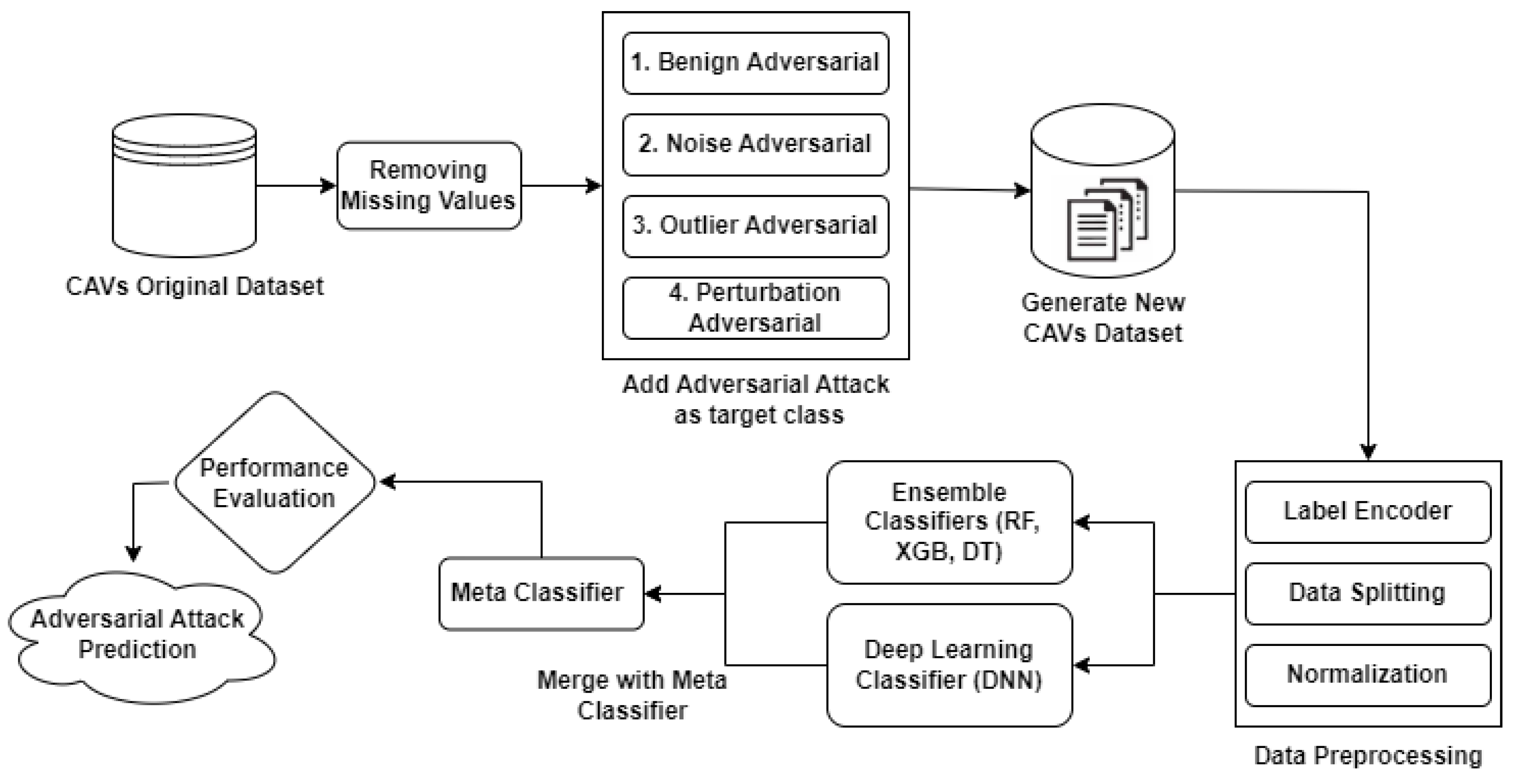
This section provided information on the proposed methodology, including all steps, such as dataset details, dataset preprocessing techniques, and network models (ML and DL classifiers) used for creating ensemble and hybrid models. Machine learning classifiers such as MLP, RF, XGB, KNN, DT, and deep learning classifiers such as DNN are the foundational elements of our suggested techniques. The working of our proposed methodology is shown in Figure 2.
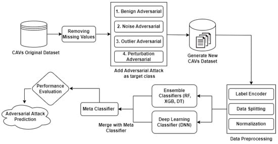
Figure 2.
Proposed model based on ML and DL classifiers.
3.1. Dataset Preliminaries
The dataset was gathered while deploying the Safety Pilot Model (SPMD). Basic safety messages (BSMs), vehicle trajectories, different driver–vehicle interaction data, and contextual data that explain the conditions under which the Model Deployment data were gathered are the data types these entities supply. Almost all of the data in this context came from roadside units and onboard vehicle devices [24]. The data collection utilized in this investigation was first investigated for anomaly identification by [11]. The three characteristics in the dataset were as follows: (i) speed, which is determined by the vehicle speedometer and is represented by sensor 1; (ii) GPS speed, which is represented by sensor 2; and (iii) acceleration, which is determined by the vehicle speedometer and is represented by sensor 3. We used an original Safety Pilot Model Deployment (SPMD) dataset [24] for this study, which is devoid of abnormalities [11].
We generated the original dataset, which has the shape (203193, 3). This section details the first step of data preprocessing.
3.1.1. Handling Missing Values
Identification: We first identified missing values in the dataset using descriptive statistics and visualization tools.
Removal: We then removed rows with missing values (NaN or None) from the DataFrame. This step resulted in a new data frame with the dimensions (30000, 3), indicating that the dataset now contains 30000 records and 3 features without any missing values.
3.1.2. Adversarial Attacks
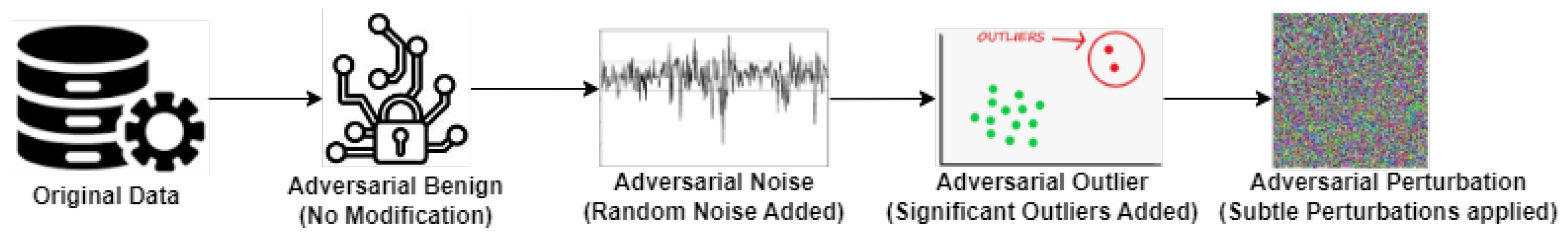
We divided the dataset into four parts to add different attacks, and every data frame had a shape of 7500. 3. Several adversarial attacks are available in the literature. Ref. [25] summarizes the taxonomy of intrusions or attacks in computer network systems, which encompass CAVs. Also, several faulty sensor behaviors are discussed in [26]. We used four types of adversarial attacks that are explained one by one below:
- Adversarial Benign: This attack represents the original, clean data without any modifications. In the context of machine learning, it refers to the normal, unperturbed instances that are typically used for training or testing models.
- Adversarial Noise Injection: In this type of attack, random Adversarial Noise Injection is added to the original data. The purpose of noise injection is to perturb the data so that it becomes more difficult for machine learning algorithms to classify or make predictions accurately. The added noise can disrupt the patterns present in the data, leading to incorrect model outputs.
- Adversarial Outlier: Outlier injection adds values to the original data. An outlier is a data point that significantly deviates from the rest of the data in the dataset. Outliers can skew statistical analyses and machine learning models, leading to inaccurate results. Outlier injection attacks aim to exploit vulnerabilities in models’ sensitivity to outliers.
- Adversarial Perturbation: Perturbation injection introduces deliberate changes or perturbations to the original data. These changes can be of various types, such as flipping the sign of feature values, adding or subtracting a small constant, or multiplying by a random factor. Perturbation injection attacks aim to deceive machine learning models by altering the input data in subtle ways that may not be immediately noticeable but can lead to incorrect predictions or classifications.
These four types of adversarial attacks demonstrate different strategies for manipulating data to deceive machine learning models, highlighting the importance of robustness and security in machine learning systems. Figure 3 presents the visualization of an adversarial attack on data.
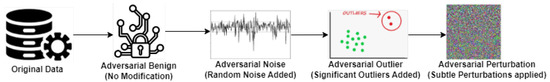
Figure 3.
Visualization of an adversarial attack.
Algorithm 1 outlines a process for generating a new dataset with adversarial attacks based on an original dataset without anomalies. The algorithm takes an original dataset without anomalies as input and aims to generate a new dataset containing adversarial attacks. The original dataset undergoes a data-cleaning process to prepare it for injecting adversarial attacks. This step might involve handling missing values. The cleaned dataset is divided into four parts to add different types of adversarial attacks. These attacks include adverse bait, noise, outlier, and perturbation. For each type of adversarial attack, a function is called to generate and add the corresponding adversarial instances to the divided parts of the dataset. After adding adversarial attacks to each part of the dataset, a function dataset merge is called to merge all datasets containing adversarial attacks into a new dataset. Finally, the algorithm returns the new dataset containing the data and adds adversarial attacks.
| Algorithm 1 Psuedo Code for Adversarial Attacks |
|
3.1.3. Label Encoder
A Label Encoder is a tool used in machine learning to convert category labels into numerical values. Many machine learning methods require the input data to be in the numerical format. A Label Encoder gives each category a distinct number in a categorical feature. Since the transformation is carried out consistently, the same category will always have the same integer encoded. We only utilized one hot label encoder in this study. One-hot encoding is a method for converting each category into a binary vector representation. Every category is assigned a distinct column; for every data point, the category-corresponding column is labeled with a 1, while all other columns are labeled with 0s. Since it avoids imposing any artificial ordering, this strategy is helpful when there is no ordinal link between the categories [27].
Assume we want to encode a single sample x with the value , where i is the category index in the categorical feature. We have a categorical feature with n categories. For sample x, the one-hot encoded vector v is expressed as follows: ....... The number of categories n equals the length of vector v. The category is represented by vector v, whose i-th element is set to 1. Vector v has all other elements set to 0.
3.1.4. Data Splitting
The dataset is divided into test, validation, and training sets to assess the interpretation of ML models. This prevents overfitting from happening and helps assess how generalizable the models are. First, we split the MI dataset into 80% training and 20% testing sets for this study. The mathematical formula used for the training and testing split is as follows:
Training Set Size
Test Set Size
The training and testing sizes are shown in Equations (1) and (2). The dataset’s total number of occurrences is D. The ratio of instances assigned to the training set is known as the train_ratio. The ratio of instances assigned to the test set is the test_ratio. Based on the given ratios, these formulae provide you with the sizes of the training and test sets. While the remaining samples implicitly determine the size of the test set after assigning to the training set, adjusting the train_ratio will directly change the size of the training set.
3.1.5. Normalization
Normalization is a data preprocessing technique used to scale feature values to a common range. This is performed because similar-scale features yield superior results for many ML and DL classifiers. To rescale the dataset features between 0 and 1, this study uses a normalizing strategy [28], which makes normalization and assembly easier. In this study, the characteristics are transformed to have a mean of 0 and a standard deviation of 1 using Z-score scaling, commonly known as standardization. For Z -score scaling, the following mathematical Equation (3) is used:
where is the feature’s standard deviation, is the dataset’s mean, and Z is the actual feature value.
3.2. Classification Models
This section explains the concepts of Multi-Layer Perceptron, Decision Tree, Random Forest, Extreme Gradient Boosting, and Deep Neural Network, which are the foundations of our suggested techniques. The classifiers are chosen according to their ability to handle various scenarios, including noisy, huge, and small datasets, and weak learning classifiers’ capacity to increase detection rates.
3.2.1. Multi-Layer Perceptron
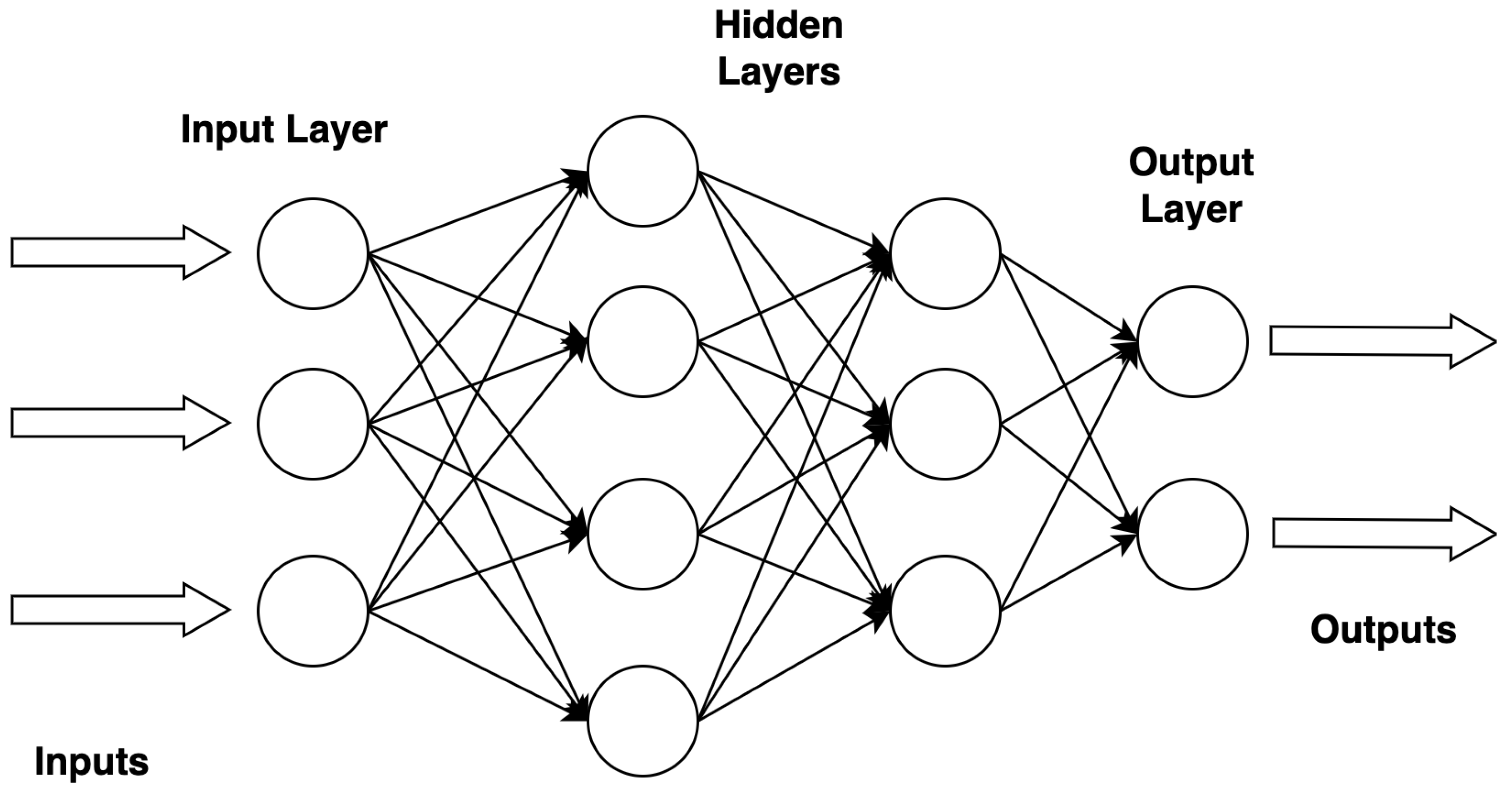
An artificial neural network (ANN) called a Multilayer Perceptron (MLP) comprises several layers of nodes, including an input layer, one or more hidden layers, and an output layer. Every node in one layer is connected to every other node, and every connection has a weight attached. The first layer of the network receives the data, which are then sent through the hidden levels, where each layer modifies the data according to the connection weights. The output layer generates the predictions or classifications the network makes at the end. MLPs are usually trained using methods like backpropagation, in which the connections’ weights are iteratively changed to reduce the discrepancy between the output obtained and the anticipated output based on a specific loss function. MLPs are the building blocks of many deep learning models and are widely utilized in ML for various tasks, including pattern recognition, regression, and classification. However, they demand a substantial amount of processing power for training, particularly when dealing with huge datasets and intricate architectures, and they may experience overfitting if they are appropriately regularized. Figure 4 displays the basic architecture of the MLP classifier.

Figure 4.
Architecture of MLP classifier.
3.2.2. Random Forest
A process known as Random Forest, which is an ensemble learning approach, creates a more accurate and dependable model by combining many decision trees [29]. Being a member of the tree-based model class, it is a well-liked model for regression and classification applications. Random Forest models, trained on bootstrapped dataset samples, independently construct several decision trees using random feature selection. It reduces variation because the model averages or uses majority voting to combine predictions from individual trees. It enhances generalization performance, making it less prone to over-fit than individual trees. Mathematically, the prediction of a Random Forest model can be represented in Equation (4) for classification:
where is the prediction of the i-th decision tree, and is the final predicted class.
3.2.3. Decision Tree
Decision Trees are supervised learning algorithms that use the provided characteristic values to inform their decisions, resulting in the creation of regions within the feature area [30]. At every node, the tree optimizes a selected criterion (e.g., data collection, Gini impurity) to determine which qualities best segregate the data. This process iterates back and forth until an end condition is satisfied, like reaching a maximum depth or a minimum number of samples per leaf. Because of their simplicity of use and capacity to handle numerical and categorical data, decision trees are utilized extensively across several industries. If appropriate regularization processes are not followed, they may overfit and have trouble generalizing to new data in big, complicated datasets. The decision tree model can be mathematically represented for classification: Let us assume denotes the decision tree model’s prediction for input x. can be represented as a function that recursively evaluates decision rules based on x features until reaching a leaf node. The predicted class for x is then determined by the majority class of the instances in the corresponding leaf node.
3.2.4. K-Nearest Neighbor
An effective supervised machine learning technique for regression and classification problems is K-Nearest Neighbors (K-NNs). It is straightforward yet highly effective. Instead of learning explicit patterns, the algorithm memorizes the training dataset in instance-based learning. In K-NN, every accessible example is stored, and new cases are categorized using a similarity metric. The algorithm determines the K-Nearest Neighbors for a given input sample from the training set and then designates the majority class among these neighbors as the input sample’s prediction. One hyperparameter that must be predetermined is the value of K.
K-NN is a non-parametric algorithm, making no assumptions about the underlying data distribution. It is also called a lazy learning algorithm because it does not explicitly learn a model during training; instead, it waits until a prediction is required. While K-NN is comfortable comprehending and executing, it can be computationally costly, especially with extensive datasets, as it needs to compute distances for each new instance to all existing instances. Additionally, choosing the value of K and the appropriate distance metric can significantly impact the algorithm’s performance. The mathematical representation of the KNN algorithm is given in Equation (5) for classification:
where is the predicted class label for the input data point x, K is the number of nearest neighbors, represents the class labels of the i-th nearest neighbor, c represents each unique class label, and 1 is the indicator function.
3.2.5. Extreme Gradient Boosting
Extreme Gradient Boosting (XGBoost) is a powerful ensemble learning method based on gradient boosting. To optimize the weak learners—typically decision trees built one after the other—gradient descent is employed [31]. XGBoost is well-known for its efficiency, scalability, and quick processing of structured and tabular data. It employs regularization strategies to prevent overfitting and has built-in capability for managing missing information. To maximize model performance, XGBoost also offers advanced features like cross-validation and early stopping.
In mathematical form, the prediction of XGBoost is represented in Equation (6):
where is the predicted output for the input data point x, N is the total number of trees in the ensemble, and represents the prediction of the i-th tree for the input x.
3.2.6. Deep Neural Network
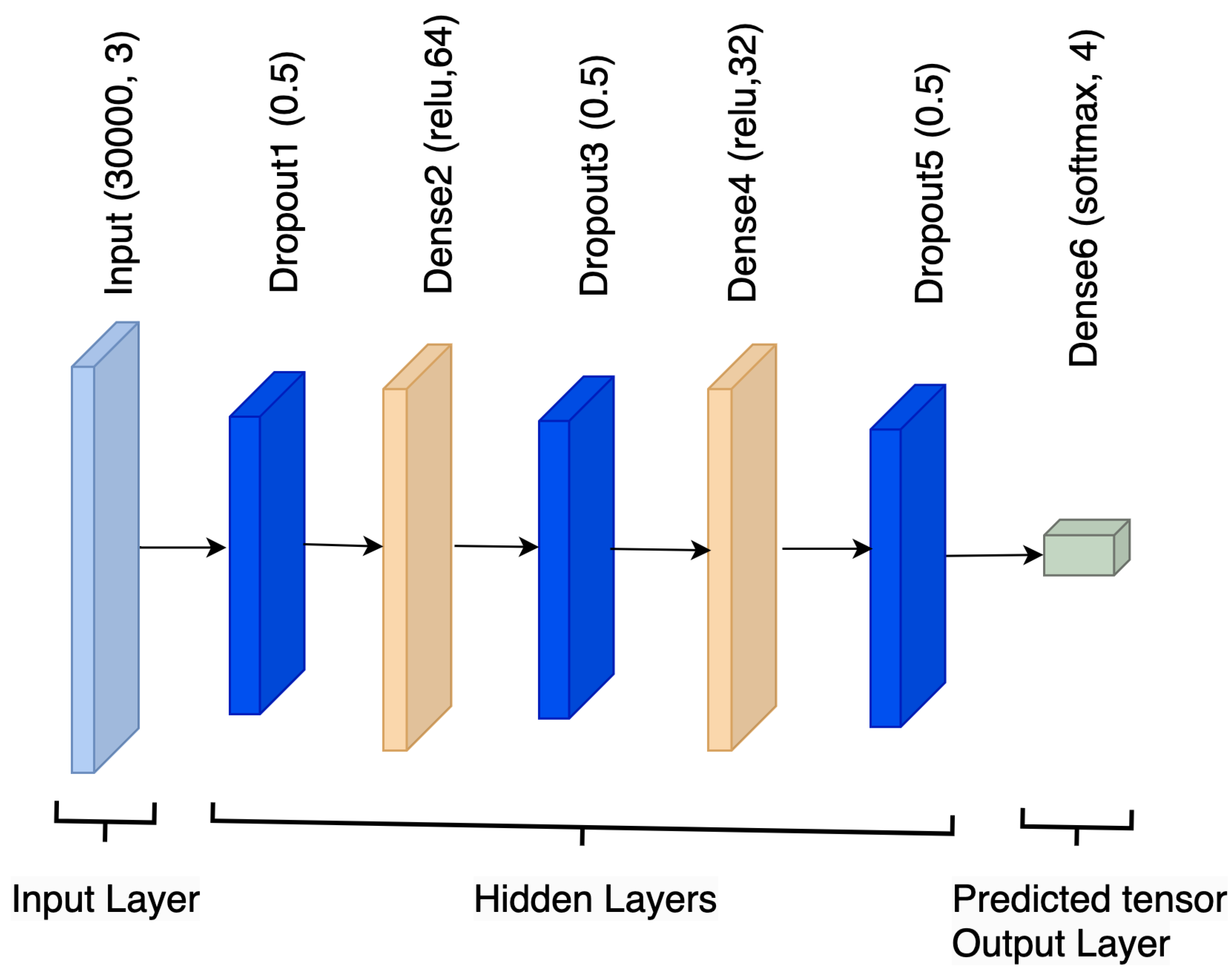
An artificial neural network with many layers of deep architecture separating the input and output layers is called a Deep Neural Network (DNN). Layers of a DNN are composed of connected nodes or neurons. These networks are capable of identifying and expressing complex hierarchical patterns and features in data. Speech recognition, computer vision, natural language processing, and many other fields have shown great interest in deep learning, of which DNNs are a crucial component. Deep learning has also shown great potential in these and other disciplines. Deep Neural Networks (DNNs) have demonstrated remarkable efficacy in independently generating hierarchical representations from data [32]. This enables DNNs to capture intricate features and connections effectively. Figure 5 shows the architecture of the DNN model.

Figure 5.
Deep neural network architecture.
DNN models predict the class labels (i.e., Normal, Adversarial Noise Injection, Adversarial Outliers, Adversarial Perturbation) based on the highest probability among the softmax probabilities generated for each class. After feeding the input data through the neural network and all processes, such as weight assignment and activation function, the model produces a vector of probabilities, each representing the probability of belonging to a particular class. The class with the highest probability is then selected as the predicted class label. The model identifies this predicted class label based on the index corresponding to the highest probability in the probability vector.
3.2.7. TAAD-CAV
This study proposes an innovative approach to enhance classification accuracy by combining traditional machine learning (ML) classifiers with a Deep Neural Network (DNN) model, augmented by a Decision Tree meta-classifier for final prediction aggregation. Initially, three distinct ML classifiers—Support Vector Classifier (SVC), Gaussian Naive Bayes (GaussianNB), and K-Nearest Neighbors (KNNs)—are individually trained on the dataset. These classifiers are integrated using a hard voting strategy within a voting classifier framework. Hard voting aggregates predictions from each base classifier, with the final prediction for each instance determined by the majority vote. This ensemble approach leverages the diverse strengths of each classifier to improve overall prediction robustness.
In parallel, a Deep Neural Network (DNN) model is trained on the same dataset to capture complex nonlinear relationships and patterns. Once trained, the DNN model independently generates predictions for the test data based on its learned representations and hierarchical feature extraction capabilities. This dual approach—combining ensemble classifiers with a deep learning model—aims to exploit the complementary advantages of both paradigms, enhancing classification performance across varied and complex datasets.
Following the generation of predictions from the ensemble classifier and the DNN model, these predictions are concatenated into a single array. This array forms a feature matrix where each row corresponds to an instance in the test set, and each column represents a prediction from either the ensemble classifiers or the DNN model. This structured data format allows for seamless integration and the comparison of predictions across different classifiers.
To consolidate and refine these diverse predictions, a Decision Tree classifier is introduced as a meta-classifier. The Decision Tree meta-classifier is trained using the concatenated predictions as features and the true labels of the training set as targets. The optimal hyperparameters, such as the maximum depth and the minimum number of samples per leaf for the Decision Tree meta-classifier, are determined through a systematic evaluation process. This involves grid search and cross-validation techniques, where the grid search systematically explores various hyperparameter combinations, and cross-validation assesses their impact on model performance. Specifically, cross-validation splits the dataset into multiple folds, trains the model on several combinations of these folds, and averages performance metrics like accuracy, precision, recall, and F1-score to ensure the robustness and generalization capability of the model. The chosen hyperparameter values maximize predictive accuracy and coherence in synthesizing outputs from diverse classifiers.
By learning to combine and weigh the outputs of the ensemble classifier and the DNN model effectively, the meta-classifier enhances prediction accuracy and generalization capabilities. This meta-learning approach ensures that the final predictions are based on a comprehensive synthesis of insights derived from both traditional ML and deep learning methodologies.
4. Experimental Result and Discussion
This section includes the evaluation measurements used to evaluate the model performance and explains the findings and results of the proposed model in detail. The efficiency of this study’s proposed model was evaluated utilizing different evaluation measurements, including accuracy, precision, recall, and F1-score and confusion matrix. Evaluation measurements were utilized to assess the prediction and classification problems.
4.1. Machine Learning Approach
Table 2 presents the performance results for the classification report for an RF classifier. Adversarial Benign had a precision of 0.61, which means 61% of instances predicted were correctly identified, and the recall value was 0.63, which means the classifier identified 63% of all actual instances of this class in the dataset. The F1-score, which balances precision and recall, for this class was 0.62. Adversarial Noise Injection had a precision of 0.73, which means 73% of instances were predicted correctly. The recall value was 0.68, which means the classifier identified 68% of all actual instances, and the F1-Score for this class was 0.70. Adversarial Outlier had a precision of 0.66, which means 66% of instances predicted as Adversarial Outlier were correct. The recall was 0.68 for this class, the classifier identified 68% of all actual instances, and the F1-score was 0.67. Adversarial Perturbation had a precision of 0.82. A total of 82% of instances predicted were correct, with a recall of 0.83 for all actual instances, and the F1-score for this class was 0.83. The Adversarial Perturbation class had the highest precision, recall, and F1 score. However, the performance for the Adversarial Benign class was the lowest among the four classes, with the lowest precision, recall, and F1 score. The model’s overall accuracy was 0.70, meaning that it correctly classified 70% of all instances across all classes. The macro-average values provide an average across all classes, with precision, recall, and F1-score being 0.71, 0.70, and 0.70, respectively. The weighted average values consider the class distribution, providing a more representative overall performance measure. In this case, the weighted average precision was 0.71, and the recall and F1-score had the same value of 0.70, reflecting the model’s performance while considering the varying numbers of instances in each class. In a classification report, “support” refers to the number of true instances for each label in the dataset. It indicates the number of occurrences of each class in the dataset that was used for evaluating the classifier.
Table 2.
Classification report for Random Forest classifier.
Table 3 presents the performance results for the classification report for the XGB classifier. Adversarial Benign had a precision, recall and F1-Score of 0.55, which means this classifier correctly identified 55% of instances predicted. Adversarial Noise Injection had a precision of 0.70, which means 70% of instances were predicted correctly. The recall value was 0.62, which means the classifier identified 62% of all actual instances, and the F1-Score for this class was 0.66. Adversarial Outlier had a precision of 0.62, which means 62% of instances predicted as Adversarial Outlier were correct. Recall was 0.71 for this class, the classifier identified 71% of all actual instances, and the F1-score was 0.66. Adversarial Perturbation had a precision of 0.82. A total 82% of the instances predicted were correct, with a recall of 0.78 for all actual instances, and the F1-score for this class was 0.80. The Adversarial Perturbation class had the highest precision, recall, and F1 score, and the Adversarial Benign class was the lowest among the four classes, with the lowest precision, recall, and F1 score. The classifier achieved an accuracy of 0.66, suggesting reasonable overall performance in classifying instances correctly. The macro-average values provide an average across all classes, with precision, recall, and F1-score being 0.67, 0.66 and 0.67, respectively. The weighted average values consider the class distribution, providing a more representative overall performance measure. In this case, the weighted average precision was 0.67, and the recall and F1-score had the same value of 0.66, reflecting the model’s performance while considering the varying numbers of instances in each class.
Table 3.
Classification report for XGB classifier.
Table 4 presents the performance results for the classification report for the KNN classifier. The Adversarial Benign class achieves a precision of 0.50, a recall of 0.62, and an F1-score of 0.55. This suggests that the classifier identified a relatively high proportion of actual instances. For the Adversarial Noise Injection class, a precision of 0.66, a recall of 0.60, and an F1-score of 0.63 are achieved. This indicates a moderate performance in identifying instances of this class with a balance between precision and recall. The KNN classifier achieves a precision of 0.67, a recall of 0.59, and an F1-score of 0.63 for the Adversarial Outlier class. Similar to the Adversarial Noise Injection class, there is a moderate balance between precision and recall. The Adversarial Perturbation class achieves a relatively higher performance with a precision of 0.80, recall of 0.76, and an F1-score of 0.78. This indicates that the classifier is quite effective in identifying Adversarial Perturbation. The Adversarial Benign class is the lowest among the four classes, with the lowest precision, recall, and F1 score. The overall accuracy of the K-Neighbors classifier is 0.64, suggesting that 64% of all instances are classified correctly across all defined classes. The macro-average precision, recall, and F1-score are 0.66, 0.64, and 0.65, respectively. The weighted average precision, recall, and F1-score are also 0.66, 0.64, and 0.65, respectively.
Table 4.
Classification report for K-Neighbors classifier.
Table 5 presents the performance results for the classification report for the DT classifier. The Adversarial has a precision of 0.60, meaning that out of all instances, 60% are predicted correctly. The recall and F1-score of 0.59 indicates that the model correctly identifies 59% of all actual instances. For the Adversarial Noise Injection class, the model performs better with a value of 0.68 for all evaluation metrics, including precision, recall and F1-score. The classifier achieves a precision of 0.64, a recall of 0.63, and an F1-score of 0.63 for the Adversarial Outlier class. In the Adversarial Perturbation class, the classifier demonstrates relatively high performance with a precision of 0.78, a recall of 0.81, and an F1-score of 0.80. This indicates that the classifier is quite effective in identifying instances of Adversarial Perturbation. The model’s overall accuracy is 0.68, meaning that it correctly classifies 68% of all instances across all classes. The macro-average values provide an average across all classes, with a 0.68 precision, recall, and F1-score value. The weighted average precision, recall, and F1-score are also 0.67, 0.68, and 0.68, respectively. A weighted average considers the support for each class, giving more weight to classes with a larger number of instances.
Table 5.
Classification report for Decision Tree classifier.
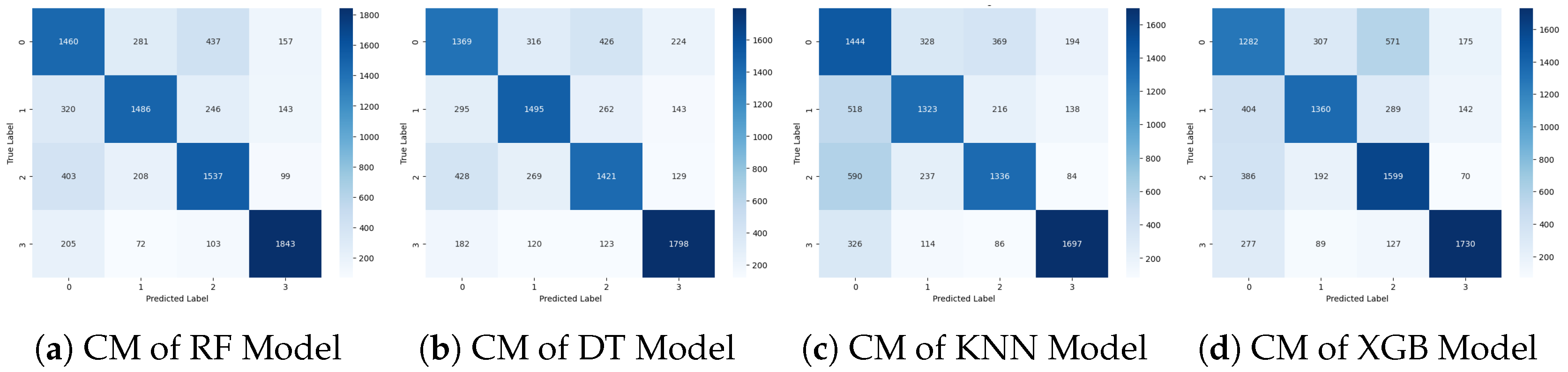
Figure 6 visualizes the confusion matrix (CM) of the ML approaches. This visualization offers a high-level overview of how the classification algorithm executes. The performance of this approach appears to be superior, as indicated by fewer false positive and false negative outcomes, along with higher counts of true positive and true negative values. The CM illustrates instances where the algorithm misclassified records, while the diagonal elements represent correct predictions. Overall, the ML approach demonstrates improved accuracy and effectiveness in classification tasks compared to traditional methods.
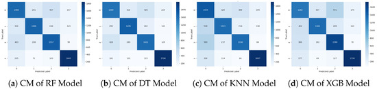
Figure 6.
Confusion matrix graphs of the machine learning approach.
4.2. Machine Learning Ensemble Approach
Table 6 presents the performance results for the classification report for the ensemble voting classifier. Adversarial Benign has a precision of 0.59, indicating that out of all instances predicted as Adversarial Benign by the classifier, only 59% are correct. It has a recall of 0.64, and the classifier identifies 64% of all instances of adversarial benign behavior in the dataset. F1-score is 0.62, which is the harmonic mean of precision and recall. Adversarial Noise Injection has a precision of 0.74, which means that 67% of instances predicted as Adversarial Noise Injection are correct, and recall with 0.67 and F1 score for this class is 0.70. Adversarial Outlier has a precision of 0.66, in which 66% of instances predicted as Adversarial Outlier are correct. The recall of this class is 0.69, in which the classifier identifies 69% of all actual instances of Adversarial Outliers in the dataset. The F1-score, which balances precision and recall for this class, is 0.68. Adversarial Perturbation has a precision of 0.84, which indicates that 84% of instances are predicted correctly, and recall has a 0.82 value, which the classifier identifies as 82% of all actual instances. The F1 score for this class is 0.83. The Adversarial Perturbation class has the highest precision, recall, and F1 score. However, the performance for the Adversarial Benign class is the lowest among the four classes, with the lowest precision, recall, and F1 score. The model’s overall accuracy is 0.70, meaning that it correctly classifies 70% of all instances across all classes. The macro-average values provide an average across all classes, with a precision and F1-score of 0.71 and recall of 0.70, respectively. The weighted average values consider the class distribution, providing a more representative overall performance measure. In this case, the weighted average precision is 0.71, and recall and F1-score are 0.70, reflecting the model’s performance while considering the varying numbers of instances in each class.
Table 6.
Classification report for ensemble classifier.
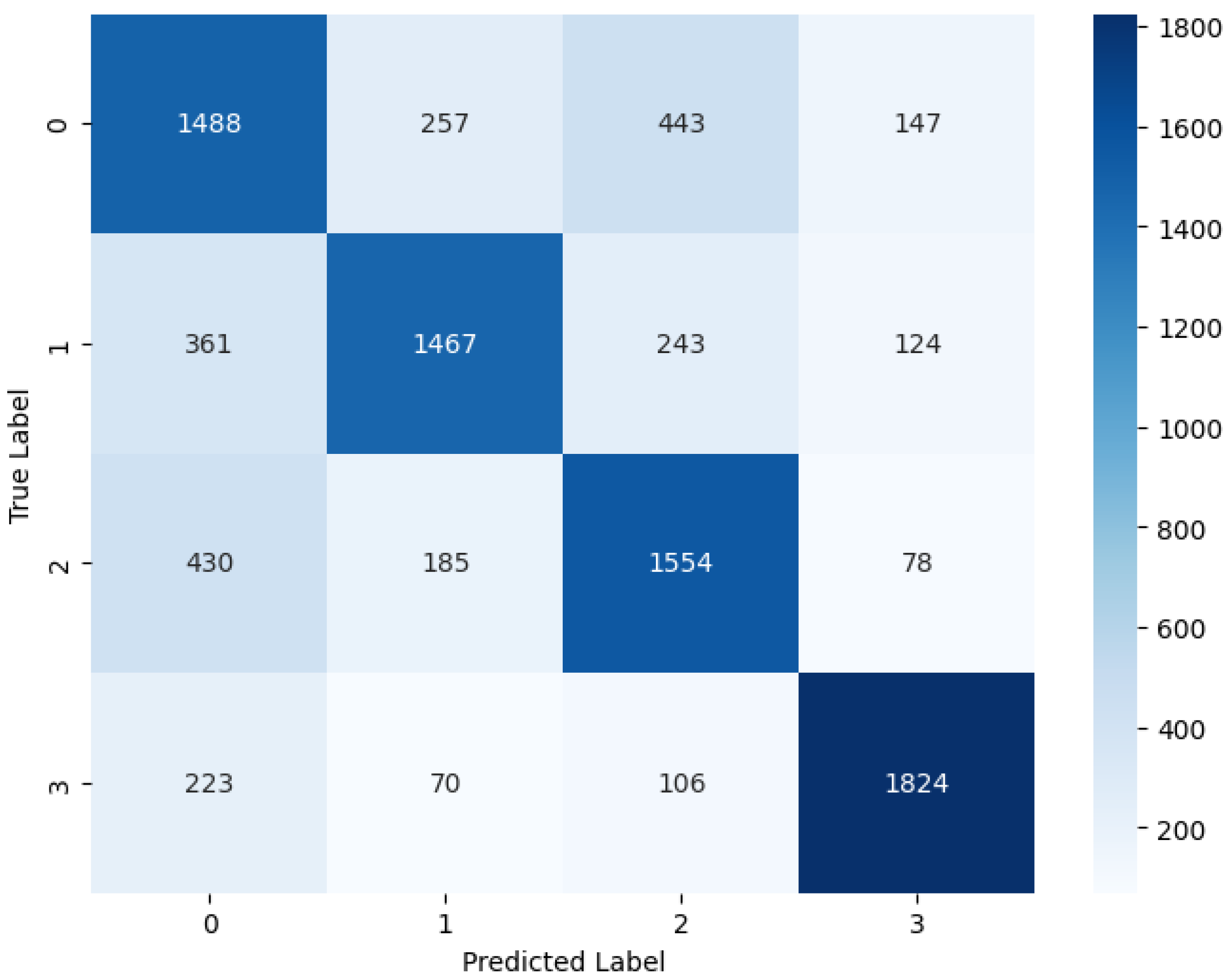
Figure 7 visualizes the CM of the ensemble voting approach. This visualization offers a high-level overview of how the classification algorithm executes. The performance of this approach appears to be superior, as indicated by fewer false positive and false negative outcomes, along with higher counts of true positive and true negative values. The CM illustrates instances where the algorithm misclassified records, while the diagonal elements represent correct predictions. Overall, the ensemble approach demonstrates improved accuracy and effectiveness in classification tasks compared to traditional methods.

Figure 7.
Confusion matrix graphs of machine learning ensemble approach.
4.3. Deep Learning Approach
Table 7 presents the performance results for the classification report for an MLP classifier. Adversarial Benign had a precision of 0.40, indicating that out of all instances predicted as Adversarial Benign by the classifier, only 40% were correct. It had a recall of 0.46, and the classifier identified 46% of all instances of adverse benign behavior in the dataset. F1-score was 0.43, which is the harmonic mean of precision and recall. For this class, it was 0.43, which balances both precision and recall. Adversarial Noise Injection had a precision of 0.67, which means that 67% of instances predicted as Adversarial Noise Injection were correct, and recall with 0.52 indicates the classifier identified 52% of all actual instances of Adversarial Noise Injection in the dataset. The F1 score for this class was 0.58. Adversarial Outlier had a precision of 0.58, in which 58% of instances predicted as Adversarial Outlier were correct. The recall of this class was 0.66, in which the classifier identified 66% of all actual instances of Adversarial Outliers in the dataset. The F1-score, which balances precision and recall for this class, was 0.62. Adversarial Perturbation had a precision of 0.79, which indicates that 79% of instances were predicted correctly, and recall had a 0.73 value, which the classifier identified as 73% of all actual instances. The F1 score for this class was 0.76. The Adversarial Perturbation class had the highest precision, recall, and F1 score. However, the performance for the Adversarial Benign class was the lowest among the four classes, with the lowest precision, recall, and F1 score. The overall accuracy of the model was 0.59, meaning that it correctly classified 59% of all instances across all classes. The macro-average values provided an average across all classes, with precision, recall, and F1-score being 0.61, 0.59, and 0.60, respectively. The weighted average values consider the class distribution, providing a more representative overall performance measure. In this case, the weighted average precision, recall, and F1-score were all 0.61, reflecting the model’s performance while considering the varying numbers of instances in each class. These metrics give equal weight to each class, regardless of its distribution in the dataset.
Table 7.
Classification report for MLP classifier.
Table 8 presents the performance results for the classification report for the DNN classifier. The DNN classifier achieves a precision of 0.39 and a recall of 0.44 for the Adversarial Benign class, resulting in an F1 score of 0.41. This indicates that the classifier correctly identifies 44% of instances belonging to the Adversarial Benign class out of all instances. For the Adversarial Noise Injection class, the classifier demonstrates a precision of 0.73, a recall of 0.49, and an F1-score of 0.58. This suggests that while the classifier achieves high precision, it may miss a significant portion of actual instances of Adversarial Noise Injection. The classifiers achieve a precision of 0.57, a recall of 0.70, and an F1-score of 0.63 for the Adversarial Outlier class. For the Adversarial Perturbation class, the classifiers demonstrate relatively high performance with a precision of 0.78, a recall of 0.74, and an F1-score of 0.76. This indicates that the classifier effectively identifies Adversarial Perturbation. The overall accuracy of the DNN classifier is 0.59, suggesting that 59% of all instances are classified correctly. The macro-average precision, recall and F1-score are 0.62, 0.59, and 0.60, respectively. The weighted average precision, recall, and F1-score are also 0.61, 0.59, and 0.59, respectively.
Table 8.
Classification report for DNN classifier.
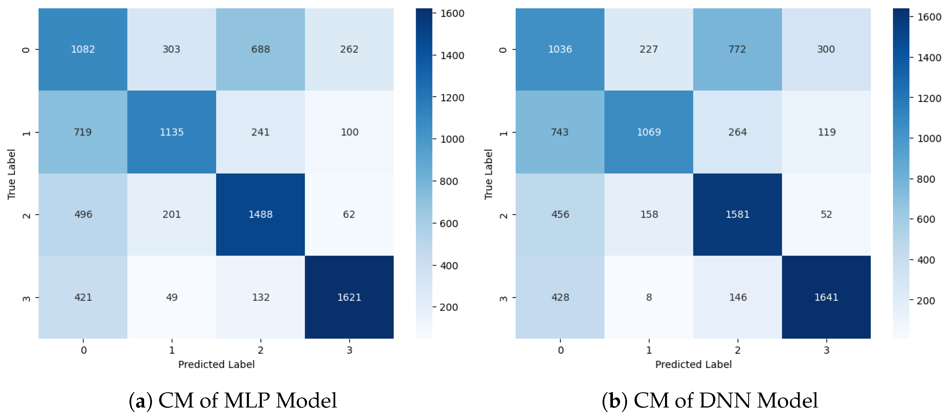
Figure 8 visualizes the CM of the DL classifiers. This visualization offers a high-level overview of how the classification algorithm executes. The performance of this approach appears to be superior, as indicated by fewer false positive and false negative outcomes, along with higher counts of true positive and true negative values. The CM illustrates instances where the algorithm misclassified records, while the diagonal elements represent correct predictions. Overall, the MLP and DNN classifiers demonstrate improved accuracy and effectiveness in classification tasks compared to traditional methods.
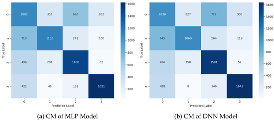
Figure 8.
Confusion Matrix Graphs of Deep Learning Approaches.
4.4. TAAD-CAV Results
Table 9 presents the performance results for the classification report for the meta classifier. The meta classifier achieves a precision of 0.59 and a recall of 0.64 for the Adversarial Benign class, resulting in an F1-score of 0.62. This indicates that 59% of instances predicted as Adversarial Benign are correct, and the classifier identifies 64% of all actual instances of Adversarial Benign in the dataset. For the Adversarial Noise Injection class, the meta classifier demonstrates a precision of 0.74, a recall of 0.67, and an F1-score of 0.70. This indicates that the classifier performs relatively well in identifying Adversarial Noise Injection instances. The classifier achieves a precision of 0.67, a recall of 0.69, and an F1-score of 0.68 for the Adversarial Outlier class. For the Perturbation Injection class, the classifier demonstrates a relatively high performance with a precision of 0.84, recall of 0.82, and an F1-score of 0.83. This indicates that the classifier is quite effective in identifying instances of Perturbation Injection. The macro-average precision, recall, and F1-score are 0.71, 0.70, and 0.71, respectively. This indicates the average performance across all classes without considering class imbalance. The weighted average precision, recall, and F1-score are also 0.71, 0.70, and 0.71, respectively. The weighted average considers the support for each class, giving more weight to classes with a larger number of instances. The meta classifier demonstrates relatively high performance across all classes, with balanced precision and recall. The classifier achieves an overall accuracy of 70%, indicating its effectiveness in classifying instances correctly across all defined classes.
Table 9.
Classification report for TAAD-CAV.
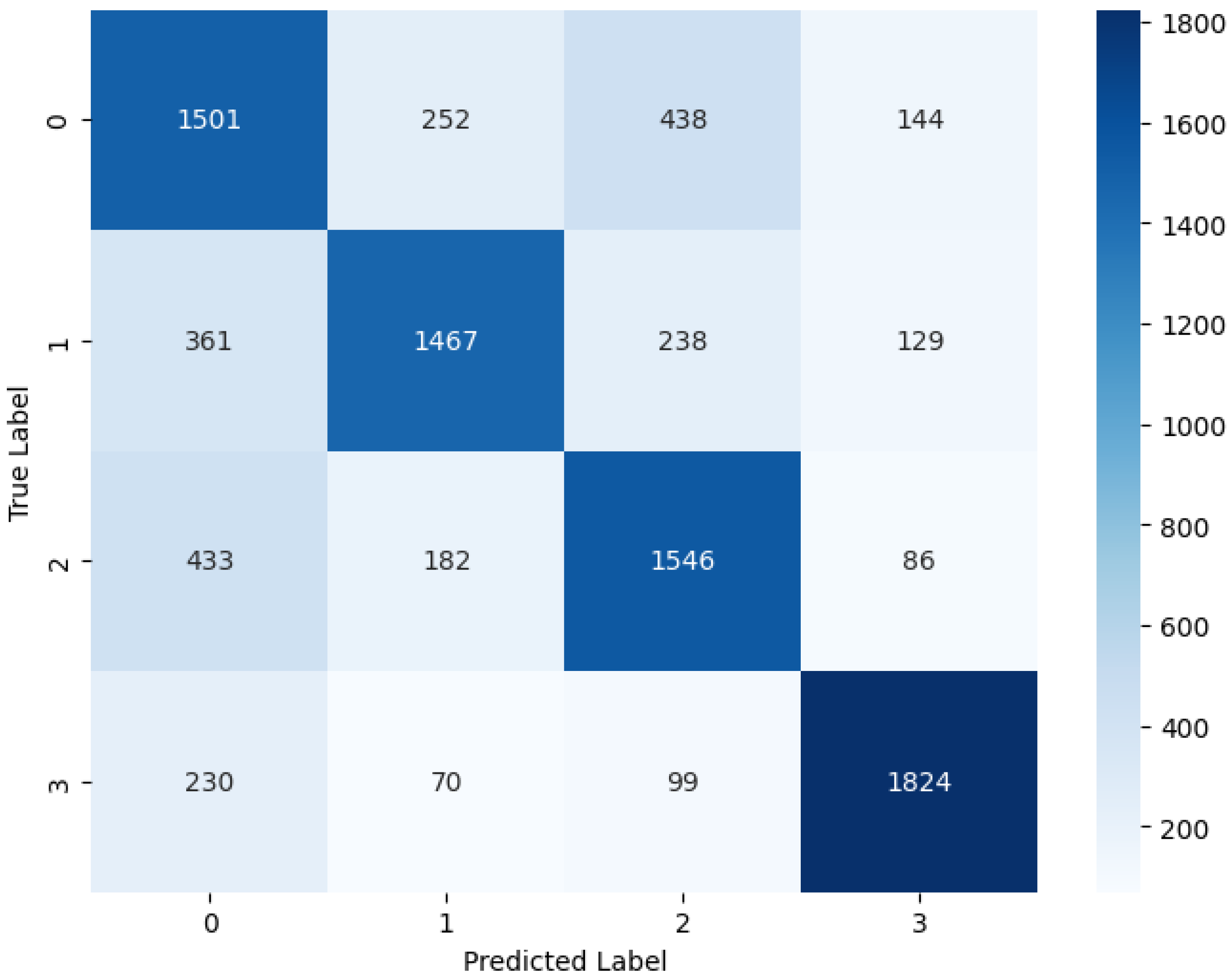
Figure 9 visualizes the CM of the hybrid ML and DL approach, which we named the Meta model. This visualization offers a high-level overview of how the classification algorithm executes. The performance of this approach appears to be superior, as indicated by fewer false positive and false negative outcomes, along with higher counts of true positive and true negative values. Overall, the Meta model demonstrates improved accuracy and effectiveness in classification tasks compared to traditional methods.
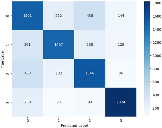
Figure 9.
Confusion matrix graphs of TAAD-CAV.
5. Deployment of TAAD-CAV
The proposed TAAD-CAV system is designed to be implemented on edge computing devices integrated within the CAV infrastructure. These edge devices, which are located either in the vehicles themselves or at roadside units, ensure minimal latency and quick response times by processing data locally. For efficient and real-time detection, we utilize powerful edge computing technologies that offer robust GPU capabilities suitable for running deep learning models. These devices provide the necessary computational power to handle the demands of the TAAD-CAV system. To ensure scalability, maintainability, and ease of updates, we employ containerization technologies like Docker. This allows the system to be easily deployed and managed across different hardware setups. The edge devices utilize secure communication protocols to send critical data to a central server for further analysis and continuous model improvement. This ensures the system remains up-to-date with the latest threat patterns. The edge devices running the TAAD-CAV system require specific hardware and software configurations. They need multi-core ARM or x86 processors, at least 16 GB of RAM to handle real-time data processing and model execution, and an NVIDIA CUDA-compatible GPU with a minimum of 4 GB of VRAM to accelerate deep learning inference. Additionally, a storage capacity of at least 256 GB SSD is necessary for fast read/write operations and to store the necessary datasets and models. The software requirements include an operating system like Ubuntu 18.04 or later, Docker for containerization, TensorFlow or PyTorch for deep learning model implementation, and Python for scripting and algorithm execution. This configuration ensures the system can operate efficiently, providing timely detection of adversarial attacks while maintaining the integrity and safety of CAVs.
6. Conclusions
To maintain vehicle and passenger safety, Connected and Automated Vehicles (CAVs) must be secured against adversarial attacks. For the safety of CAVs, it is essential to accurately and promptly recognize attacks. Considering this problem, this study proposes an adversarial attack detection hybrid technique integrating machine (RF, DT, XGB) and deep (DNN) learning classifiers with meta classifiers (e.g., Decision tree) to generate a hybrid model. This research generates a dataset without anomalies and adds adversarial attacks as a label class to create a new dataset for prediction. The following actions are taken to preprocess the dataset: the data are cleaned, labeled, divided, and normalized using Z-score normalization techniques; missing values are eliminated; the one-hot encoding method is applied; and data are split. The performance of the proposed models is evaluated utilizing accuracy, recall, precision, the F1-score, and the confusion matrix. The meta classifier is a hybrid of ML and DL models that achieves the highest performance in all models with a value of 70% accuracy. To support the findings of our suggested framework, we want to develop and examine different methodologies in further work. In the future, we will also check the generalizability of newly created dataset-based adversarial attacks by applying different machine learning, deep learning, and feature optimization techniques.
Author Contributions
Conceptualization, T.H.K., G.A.S. and M.K.; Data curation, M.A.A.; Formal analysis, T.H.K. and G.A.S.; Funding acquisition; Investigation, M.A.A., M.K., T.H.K. and G.A.S.; Methodology, M.A.A., M.K., T.H.K. and G.A.S.; Project administration, M.A.A.; Software, T.H.K. and G.A.S.; Supervision; Validation, M.A.A.; Visualization; Writing—original draft, T.H.K., G.A.S. and M.A.A.; Writing—review and editing, M.K., T.H.K., G.A.S. and M.A.A. All authors have read and agreed to the published version of the manuscript.
Funding
This research received no external funding.
Data Availability Statement
The raw data supporting the conclusions of this article will be made available by the authors on request.
Acknowledgments
Authors would like to acknowledge Princess Nourah bint Abdulrahman University Researchers Supporting Project number (PNURSP2024R503), Princess Nourah Bint Abdul Rahman University, Riyadh, Saudi Arabia.
Conflicts of Interest
The authors share no conflicts of interest.
References
- Dilek, E.; Dener, M. Computer vision applications in intelligent transportation systems: A survey. Sensors 2023, 23, 2938. [Google Scholar] [CrossRef] [PubMed]
- Lin, H.; Liu, Y.; Li, S.; Qu, X. How generative adversarial networks promote the development of intelligent transportation systems: A survey. IEEE/CAA J. Autom. Sin. 2023, 10, 1781–1796. [Google Scholar] [CrossRef]
- Tao, F.; Chen, J. Deep learning for intelligent transportation systems: A survey. IEEE Trans. Intell. Transp. Syst. 2018, 20, 4811–4826. [Google Scholar]
- Baccari, S.; Touati, H.; Hadded, M.; Muhlethaler, P. Performance Impact Analysis of Security Attacks on Cross-Layer Routing Protocols in Vehicular Ad hoc Networks. In Proceedings of the 2020 International Conference on Software, Telecommunications and Computer Networks (SoftCOM), Split, Croatia, 17–19 September 2020; pp. 1–6. [Google Scholar]
- Damaj, I.W.; Yousafzai, J.K.; Mouftah, H.T. Future trends in connected and autonomous vehicles: Enabling communications and processing technologies. IEEE Access 2022, 10, 42334–42345. [Google Scholar] [CrossRef]
- Ahangar, M.N.; Ahmed, Q.Z.; Khan, F.A.; Hafeez, M. A survey of autonomous vehicles: Enabling communication technologies and challenges. Sensors 2021, 21, 706. [Google Scholar] [CrossRef] [PubMed]
- Hadded, M.; Merdrignac, P.; Duhamel, S.; Shagdar, O. Security attacks impact for collective perception based roadside assistance: A study of a highway on-ramp merging case. In Proceedings of the 2020 International Wireless Communications and Mobile Computing (IWCMC), Limassol, Cyprus, 15–19 June 2020; pp. 1284–1289. [Google Scholar]
- Ye, X.; Zhou, J.; Li, Y.; Cao, M.; Chen, D.; Qin, Z. A location privacy protection scheme for convoy driving in autonomous driving era. Peer-Peer Netw. Appl. 2021, 14, 1388–1400. [Google Scholar] [CrossRef]
- Qayyum, A.; Usama, M.; Qadir, J.; Al-Fuqaha, A. Securing connected & autonomous vehicles: Challenges posed by adversarial machine learning and the way forward. IEEE Commun. Surv. Tutor. 2020, 22, 998–1026. [Google Scholar]
- Wang, J.; Zhang, L.; Huang, Y.; Zhao, J.; Bella, F. Safety of autonomous vehicles. J. Adv. Transp. 2020, 2020, 8867757. [Google Scholar] [CrossRef]
- Van Wyk, F.; Wang, Y.; Khojandi, A.; Masoud, N. Real-time sensor anomaly detection and identification in automated vehicles. IEEE Trans. Intell. Transp. Syst. 2019, 21, 1264–1276. [Google Scholar] [CrossRef]
- Wang, Y.; Masoud, N.; Khojandi, A. Real-time sensor anomaly detection and recovery in connected automated vehicle sensors. IEEE Trans. Intell. Transp. Syst. 2020, 22, 1411–1421. [Google Scholar] [CrossRef]
- Lee, S.; Cho, Y.; Min, B.C. Attack-aware multi-sensor integration algorithm for autonomous vehicle navigation systems. In Proceedings of the 2017 IEEE International Conference on Systems, Man, and Cybernetics (SMC), Banff, AB, Canada, 5–8 October 2017; pp. 3739–3744. [Google Scholar]
- van Wyk, F.; Khojandi, A.; Masoud, N. A path towards understanding factors affecting crash severity in autonomous vehicles using current naturalistic driving data. In Intelligent Systems and Applications, Proceedings of the 2019 Intelligent Systems Conference (IntelliSys), London, UK, 5–6 September 2019; Springer: Berlin/Heidelberg, Germany, 2020; Volume 2, pp. 106–120. [Google Scholar]
- Albahri, A.; Hamid, R.A.; Abdulnabi, A.R.; Albahri, O.; Alamoodi, A.; Deveci, M.; Pedrycz, W.; Alzubaidi, L.; Santamaría, J.; Gu, Y. Fuzzy decision-making framework for explainable golden multi-machine learning models for real-time adversarial attack detection in Vehicular Ad-hoc Networks. Inf. Fusion 2024, 105, 102208. [Google Scholar] [CrossRef]
- Zhou, M.; Che, X. Stealthy attack detection based on controlled invariant subspace for autonomous vehicles. Comput. Secur. 2024, 137, 103635. [Google Scholar] [CrossRef]
- Nazaruddin, S.A.; Chaudhry, U.B. A Machine Learning Based Approach to Detect Cyber-Attacks on Connected and Autonomous Vehicles (CAVs). In Wireless Networks: Cyber Security Threats and Countermeasures; Springer: Berlin/Heidelberg, Germany, 2023; pp. 165–203. [Google Scholar]
- Yao, Y.; Zhao, J.; Li, Z.; Cheng, X.; Wu, L. Jamming and Eavesdropping Defense Scheme Based on Deep Reinforcement Learning in Autonomous Vehicle Networks. IEEE Trans. Inf. Forensics Secur. 2023, 18, 1211–1224. [Google Scholar] [CrossRef]
- Hossain, M.Z.; Imteaj, A.; Zaman, S.; Shahid, A.R.; Talukder, S.; Amini, M.H. FLID: Intrusion Attack and Defense Mechanism for Federated Learning Empowered Connected Autonomous Vehicles (CAVs) Application. In Proceedings of the 2023 IEEE Conference on Dependable and Secure Computing (DSC), Tampa, FL, USA, 7–9 November 2023; pp. 1–8. [Google Scholar]
- Liu, Q.; Shen, H.; Sen, T.; Ning, R. Time-Series Misalignment Aware DNN Adversarial Attacks for Connected Autonomous Vehicles. In Proceedings of the 2023 IEEE 20th International Conference on Mobile Ad Hoc and Smart Systems (MASS), Toronto, ON, Canada, 25–27 September 2023; pp. 261–269. [Google Scholar]
- Cui, C.; Du, H.; Jia, Z.; Zhang, X.; He, Y.; Yang, Y. Data Poisoning Attacks with Hybrid Particle Swarm Optimization Algorithms against Federated Learning in Connected and Autonomous Vehicles. IEEE Access 2023, 11, 136361–136369. [Google Scholar] [CrossRef]
- He, Q.; Meng, X.; Qu, R.; Xi, R. Machine learning-based detection for cyber security attacks on connected and autonomous vehicles. Mathematics 2020, 8, 1311. [Google Scholar] [CrossRef]
- Sharma, P.; Austin, D.; Liu, H. Attacks on machine learning: Adversarial examples in connected and autonomous vehicles. In Proceedings of the 2019 IEEE International Symposium on Technologies for Homeland Security (HST), Woburn, MA, USA, 5–6 November 2019; pp. 1–7. [Google Scholar]
- Bezzina, D.; Sayer, J. Safety Pilot Model Deployment: Test Conductor Team Report; Report No. DOT HS 812 171; National Highway Traffic Safety Administration: Washington, DC, USA, 2015; p. 18.
- Bhuyan, M.H.; Bhattacharyya, D.K.; Kalita, J.K. Network anomaly detection: Methods, systems and tools. IEEE Commun. Surv. Tutor. 2013, 16, 303–336. [Google Scholar] [CrossRef]
- Sharma, A.B.; Golubchik, L.; Govindan, R. Sensor faults: Detection methods and prevalence in real-world datasets. ACM Trans. Sens. Netw. (TOSN) 2010, 6, 1–39. [Google Scholar] [CrossRef]
- Rodríguez, P.; Bautista, M.A.; Gonzalez, J.; Escalera, S. Beyond one-hot encoding: Lower dimensional target embedding. Image Vis. Comput. 2018, 75, 21–31. [Google Scholar] [CrossRef]
- Henderi, H.; Wahyuningsih, T.; Rahwanto, E. Comparison of Min-Max normalization and Z-Score Normalization in the K-nearest neighbor (kNN) Algorithm to Test the Accuracy of Types of Breast Cancer. Int. J. Inform. Inf. Syst. 2021, 4, 13–20. [Google Scholar] [CrossRef]
- Rigatti, S.J. Random forest. J. Insur. Med. 2017, 47, 31–39. [Google Scholar] [CrossRef]
- Song, Y.Y.; Ying, L. Decision tree methods: Applications for classification and prediction. Shanghai Arch. Psychiatry 2015, 27, 130. [Google Scholar] [PubMed]
- Chen, T.; He, T.; Benesty, M.; Khotilovich, V.; Tang, Y.; Cho, H.; Chen, K.; Mitchell, R.; Cano, I.; Zhou, T.; et al. XGBoost: Extreme Gradient Boosting; R Package Version 0.4-2; 2015; Volume 1, pp. 1–4. [Google Scholar]
- Chen, Y.; Luo, T.; Liu, S.; Zhang, S.; He, L.; Wang, J.; Li, L.; Chen, T.; Xu, Z.; Sun, N.; et al. Dadiannao: A machine-learning supercomputer. In Proceedings of the 2014 47th Annual IEEE/ACM International Symposium on Microarchitecture, Cambridge, UK, 13–17 December 2014; pp. 609–622. [Google Scholar]
Disclaimer/Publisher’s Note: The statements, opinions and data contained in all publications are solely those of the individual author(s) and contributor(s) and not of MDPI and/or the editor(s). MDPI and/or the editor(s) disclaim responsibility for any injury to people or property resulting from any ideas, methods, instructions or products referred to in the content. |
© 2024 by the authors. Licensee MDPI, Basel, Switzerland. This article is an open access article distributed under the terms and conditions of the Creative Commons Attribution (CC BY) license (https://creativecommons.org/licenses/by/4.0/).