Adaptive Multi-Surface Sliding Mode Control with Radial Basis Function Neural Networks and Reinforcement Learning for Multirotor Slung Load Systems

Abstract

While using multirotor UAVs for transport of suspended payloads, there is a need for stability along the desired path, in addition to avoidance of any excessive payload oscillations, and a good level of precision in maintaining the desired path of the vehicle. However, due to the nonlinear and underactuated nature of the system, in addition to the presence of mismatched uncertainties, the development of a control system for this application poses an interesting research problem. This paper proposes a control architecture for a multirotor slung load system by integrating a Multi-Surface Sliding Mode Control, aided by a Radial Basis Function Neural Network, with a Deep Q-Network Reinforcement Learning agent. The former will be used to ensure asymptotic tracking stability, while the latter will be used to suppress payload oscillations. First, we will present the dynamics of a multirotor slung load system, represented here as a quadrotor with a single pendulum load suspended from it. We will then propose a control method in which a multi-surface sliding mode controller, based on an adaptive RBF Neural Network for trajectory tracking of the quadrotor, works in tandem with a Deep Q-Network Reinforcement Learning agent whose reward function aims to suppress the oscillations of the single pendulum slung load. Simulation results demonstrate the effectiveness and potential of the proposed approach in achieving precise and reliable control of multirotor slung load systems.

1. Introduction

1.1. Background

Unmanned Aerial Vehicles (UAVs) have been applied in a variety of fields [1]. One of the most well-known applications is the transport of suspended payloads, which can be in the form of parcel delivery, military rescue, surveillance systems, etc. UAVs are particularly beneficial for this purpose, owing to their versatility, adaptability, and efficiency. Slung load UAVs are capable of carrying payloads suspended beneath the aircraft, enabling the transportation of goods to remote or inaccessible areas with effective agility and speed. However, the dynamics of slung load systems introduce unique challenges that must be addressed to ensure safe and efficient operation. The combination of UAVs with slung loads poses an interesting control problem. A multirotor UAV is underactuated [2], in that it has more degrees of freedom than the number of control inputs available to us. The addition of this slung load adds further degrees of freedom to the system, only increasing the complexity of the problem. The slung load also has its own complexities such as load oscillations, aerodynamic disturbances, and dynamic instabilities, all of which significantly impact the UAV’s flight performance and the safety of the payload it transports.

In recent years, to handle this problem, various control methods have been sought by researchers. In [3], a backstepping technique was introduced to manage the dynamics of a quadrotor carrying a suspended load with limited actuators. The focus was on tackling the challenge of accurately following desired trajectories for the hanging payload. The research outlined in [4] utilized Fractional Order Sliding Mode Control (FOSMC) to improve the performance of a quadrotor tracking a predefined trajectory, adding to existing knowledge by developing a resilient FOSMC strategy for quadrotors to also handle external disturbances. In [5], an approach of Nonlinear Proportional–Integral–Derivative (NLPID) controllers for position response was combined with PID controllers to handle the attitude and swing response of a coupled UAV system. The authors of [6] explored an adaptive neural network-based fault-tolerant control method tailored for quadcopter slug load systems, looking to account for perturbances such as actuator faults, wind disturbances, and the presence of a suspended payload. A double active disturbance rejection control (ADRC) strategy was suggested in [7], in which the control system incorporated an extended state observer (ESO) in both the position and attitude loops to accurately estimate and counteract system disturbances. The authors of [8] studied an axially moving helicopter slung load system, by employing a fuzzy logic system (FLS). A fuzzy control technique was utilized to atone for system uncertainties and fault deviation vectors, after which an adaptive fuzzy control law was crafted within the introduced FLS framework. In [9], a geometric finite-time inner–outer-loop control approach was introduced for quadrotor slung load systems. This strategy involved a two-loop feedback control system. The inner-loop control law focused on achieving finite-time attitude tracking for the quadrotor, while the outer-loop controller stabilized the cable direction, aiming to ensure precise tracking of the payload trajectory. In [10], an Adaptive LQR controller was introduced, where the controller’s objective focused on regulating an arbitrary point, specifically the geometric centroid of the quadcopter, rather than that of the payload or the quadcopter’s center of gravity. In [11], a backstepping technique, accompanied by the introduction of an Uncertainty and Disturbance Estimator (UDE), was developed. The UDE was noted for its ability to transform the robust control challenge into a low-pass filter design in the frequency domain, thereby producing an estimation of lumped uncertainties.

1.2. Overview

In the case of multirotor UAVs with slung loads, most existing control methods consider the application of a robust control method, which primarily focuses on the trajectory tracking control of the multirotor, while using methods such as disturbance rejection or fault tolerance for any mismatched uncertainties, including those of slung load oscillations. Reinforcement learning methods are known to be effective in the stabilization of pendula attached to moving vehicles, although these have primarily focused on inverted or rotating pendula. With the benefits of robust trajectory tracking control, and the effectiveness of a self-learning reinforcement learning (RL) controller, there is potential to produce an efficient controller which can suppress payload oscillations for any given trajectory of the multirotor.

RL has previously been implemented with robust controllers, such as model predictive control for autonomous vehicles [12], sliding mode control for PV system grid integration [13], PID for a dynamic positioning system [14], LQR for continuous-time systems [15], and also some adaptive control methods [16,17]. In these cases, however, the RL techniques are applied to the robust controllers themselves, such that the control parameters—for instance, the P, I, and D parameters of a PID controller [18]—are adjusted by an RL algorithm based on feedback received from the system it is applied to. They have not commonly been used alongside robust control methods, and their application to slung load pendulum systems is still in its early stages.

Deep Q-Network (DQN) is an RL agent that combines the principles of reinforcement learning with deep neural networks, enabling the training of agents to make high-level decisions in environments with large state and action spaces. At its core, DQN is built upon the Q-learning algorithm, a classic reinforcement learning technique. The fundamental idea behind DQN is to approximate the optimal action-value function using a deep neural network. The use of deep neural networks allows DQN to handle complex and high-dimensional input spaces effectively [19,20,21,22]. DQN has also proven to be effective in applications involving drones, such as autonomous navigation [23], parcel delivery [24], and surveillance systems [25]. Some work implementing DQN agents for the control of inverted pendula presently exists [26,27,28], although no existing work has been carried out for slung load systems, or for multilink pendula. Some research has been carried out with UAVs [29,30], although as is the case with RL, this does not include slung load transport.

Multi-Surface Sliding Mode Control (MSSC) is a variation of sliding mode control which was suggested as a means of simplifying the development of control systems with complexity in model differentiation [31]. MSSC divides a system into several smaller parts based on their structural characteristics, with each sub-part having an individual sliding surface. An MSSC system is broken down into smaller subsystems based on their characteristics, with each subsystem having an independent sliding mode surface. In recent times, MSSC has emerged as a highly promising approach in control methodology. Unlike traditional sliding mode control, where a single sliding surface guides the system’s states along a desired trajectory, MSSC divides the control space into multiple sliding surfaces. This innovation addresses challenges such as uncertainties, disturbances, and nonlinearities that can lead to performance issues in conventional methods. Researchers have explored MSSC applications across a range of fields including robotics, aerospace, automotive, and power systems [32,33].

While a conventional MSSC is effective in maintaining effective control of the system, both in terms of trajectory tracking and suppression of oscillations, there is potential for it to be improved. The integration of RBF Neural Networks (RBFNNs) with MSSC enhances the robustness and adaptability of the control system, as RBFNNs are utilized to approximate and compensate for the uncertainties and nonlinearities in the MSL, while the MSSC can maintain the system’s trajectory. Furthermore, the use of DQN-based RL introduces an adaptive element to the control strategy, which enables the slung load pendulum to learn optimal control policies through interaction with the environment, thus improving performance over time, particularly in scenarios where the system dynamics may change or where there are varying operational conditions.

There is presently an attempt to shift industrial applications such as load delivery and transport to methods which are more effective and efficient in terms of time and labor. These include the replacement of urban trucks for such operations with drones [34], healthcare delivery [35], and agriculture [36], and utilizing modern advancements in aerial vehicles, such as eVTOLs, for intelligent transportation systems [37]. With the advent of these intelligent systems, a control method to support such systems in the presence of unexpected disturbances would prove to be very useful.

Keeping these factors in mind, in this work, we will combine the benefits of both the robust MSSC and the self-learning DQN-based RL methods. We will present a framework wherein an MSSC, aided by a Radial Basis Function Neural Network (RBFNN), will be used to guarantee asymptotic stability of the multirotor UAV, while the RL agent will be applied to the suppression of the slung load oscillations. The main contributions of this paper are as follows:

(i)

Investigation of an RBFNN-MSSC applied to a thrust-vectored multirotor for trajectory tracking purposes;

(ii)

Application of a DQN-based RL agent to a slung load pendulum;

(iii)

Comparison of the performance of the combined control system with an RBFNN-MSSC applied to the entire multirotor slung load (MSL) system, based on the slung load oscillations.

2. Methodology

2.1. Dynamic Modeling

In this section, we propose a dynamic model for our multirotor slung load system, cascading their dynamics into a unified system. We use two state vectors to describe this system: $q_{trans}=[x,y,z,{\theta }_x,{\theta }_y]$ represents the system’s translational motion—with $x,y$ and $z$ denoting the position, and ${\theta }_x$ and ${\theta }_y$ denoting the slung load oscillation angles—and $q_{rot}=\left[\varphi ,\theta ,\psi \right]$. The overall state vector $q=[q_{trans},q_{rot}]$ encompasses the overall state vector. We take $M$ to be the multirotor mass and $m$ to be the slung load mass.

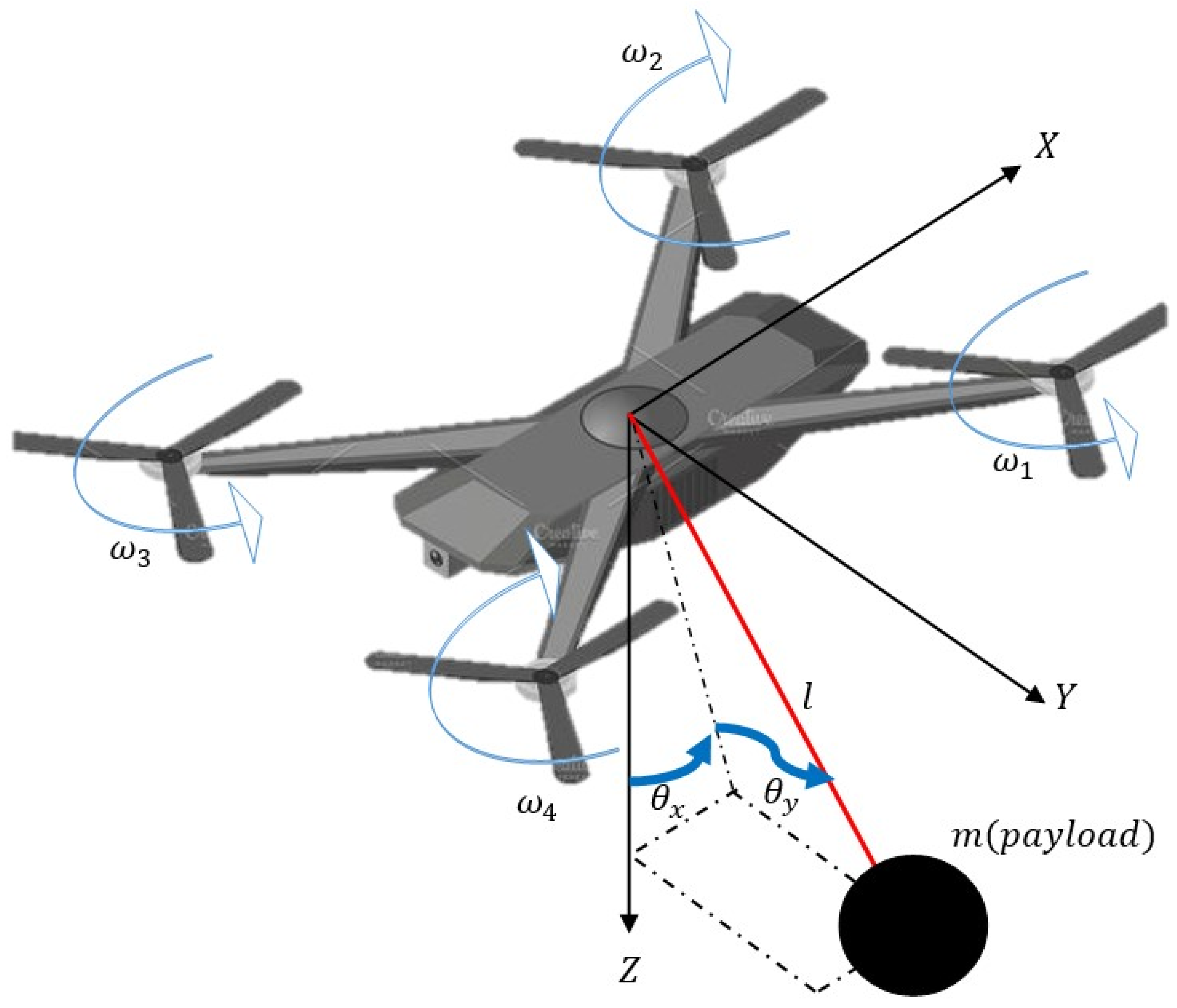
2.1.1. Multirotor Dynamics

For this work, we will consider a quadcopter with 4 rotors as our multirotor. The characteristics of this system are highlighted in Figure 1. In the following equations, $R_A^B$ will denote the rotation of some frame B into another frame A. This procedure is well documented in the literature [38].

$$\begin{gathered} R_X\left(\theta \right)=\left[\begin{array}{ccc}1& 0& 0\\ 0& C\left(\theta \right)& -S\left(\theta \right)\\ 0& S\left(\theta \right)& C\left(\theta \right)\end{array}\right] \\ {R}_y\left(\theta \right)=\left[\begin{array}{ccc}C\left(\theta \right)& 0& S\left(\theta \right)\\ 0& 1& 0\\ -S\left(\theta \right)& 0& C\left(\theta \right)\end{array}\right] \\ {R}_z\left(\theta \right)=\left[\begin{array}{ccc}C\left(\theta \right)& -S\left(\theta \right)& 0\\ S\left(\theta \right)& C\left(\theta \right)& 0\\ 0& 0& 1\end{array}\right] \end{gathered}$$

(1)

Here, $C\left(\theta \right)=cos\theta$ and $S\left(\theta \right)=sin\theta$. These represent the general rotation matrices of the multirotor in terms of its roll, pitch, and yaw.

$$\begin{gathered} R_{Pi}^b=R_Z\left(\frac{\left(i-1\right)}{2}\pi \right)R_X\left(A_i\right)R_Y\left(B_i\right) \\ =\left[\begin{array}{ccc}{R}_{{P_i}_{11}}^b& R_{{P_i}_{12}}^b& R_{{P_i}_{13}}^b\\ R_{{P_i}_{21}}^b& R_{{P_i}_{22}}^b& R_{{P_i}_{23}}^b\\ R_{{P_i}_{31}}^b& R_{{P_i}_{32}}^b& R_{{P_i}_{33}}^b\end{array}\right] \end{gathered}$$

(2)

where

$$\begin{gathered} R_{{P_i}_{11}}^b=C_{\left(\frac{\left(i-1\right)}{2}\right)\pi }{C}_{B_i}-S_{\left(\frac{\left(i-1\right)}{2}\right)\pi }{S}_{\left(A_i\right)}{S}_{\left(B_i\right)} \\ {R}_{{P_i}_{12}}^b={-S}_{\left(\frac{\left(i-1\right)}{2}\right)\pi }{C}_{\left(A_i\right)} \\ {R}_{{P_i}_{13}}^b=C_{\left(\frac{\left(i-1\right)}{2}\right)\pi }{S}_{\left(B_i\right)}+S_{\left(\frac{\left(i-1\right)}{2}\right)\pi }{S}_{{(A}_i)}{C}_{\left(B_i\right)} \\ {R}_{{P_i}_{21}}^b=S_{\left(\frac{\left(i-1\right)}{2}\right)\pi }{C}_{{(B}_i)}+C_{\left(\frac{\left(i-1\right)}{2}\right)\pi }{S}_{\left(A_i\right)}{S}_{\left(B_i\right)} \\ {R}_{{P_i}_{22}}^b=C_{\left(\frac{\left(i-1\right)}{2}\right)\pi }{C}_{{(A}_i)} \\ {R}_{{P_i}_{23}}^b=S_{\left(\frac{\left(i-1\right)}{2}\right)\pi }{S}_{\left(B_i\right)}-C_{\left(\frac{\left(i-1\right)}{2}\right)\pi }{S}_{\left(A_i\right)}{C}_{\left(B_i\right)} \\ {R}_{{P_i}_{31}}^b=-C_{\left(\frac{\left(i-1\right)}{2}\right)\pi }{S}_{\left(B_i\right)} \\ {R}_{{P_i}_{32}}^b=S_{\left(A_i\right)} \\ {R}_{{P_i}_{33}}^b=C_{\left(A_i\right)}{C}_{\left(B_i\right)} \end{gathered}$$

(3)

$$\begin{array}{l}{O}_{P_i}^b=R_Z\left(\frac{i-1}{2}\right)\pi \left[\begin{array}{c}L\\ 0\\ 0\end{array}\right]\\ =\left[\begin{array}{c}{C}_{\left(\frac{\left(i-1\right)}{2}\pi \right)L}\\ S_{\left(\frac{\left(i-1\right)}{2}\pi \right)L}\\ 0\end{array}\right]\end{array}$$

(4)

where i = 1…, n (for this quadrotor, n = 4), and L is the arm length of the multirotor, measured from the body frame centre ($O_b)$ to the center of a propeller ($O_{P_i}^b$). The torque acting on any propeller $i$, denoted as ${{\tau }_p}_i$, is first obtained using Euler’s angular momentum theory:

$${{\tau }_p}_i={I_P}_{i\dot{\omega }{P}_i}+{{\omega }_P}_i\times {I_P}_i{{\omega }_P}_i+{\left[\begin{array}{ccc}0& 0& k_c{\omega }_{P_{iZ}}\left|{\omega }_{P_{iZ}}\right|\end{array}\right]}^T$$

(5)

where ${I_P}_i$ represents each propeller’s inertia matrix, ${{\omega }_P}_{iZ}$ denotes the vector ${\omega }_{P_i}$’s z-axis component, $k_c>0$, the modulus of elasticity between ${{\omega }_P}_{iZ}$ and the counter-rotating torque about ${Z_P}_i$ axis,

$${{\omega }_P}_i={R_P}_i^{b-1}{\omega }_b+\left[\begin{array}{c}\dot{{\alpha }_{\dot{i}}}\\ \dot{{\beta }_i}\\ \widehat{{\omega }_i}\end{array}\right]$$

(6)

and $\widehat{{\omega }_i}$ is the angular velocity of the $i^{th}$ propeller. If ${T_P}_i$ is the $i^{th}$ propeller’s produced thrust, we obtain

$${T_P}_i={\left[\begin{array}{ccc}0& 0& k_f\widehat{{\omega }_i}\left|\widehat{{\omega }_i}\right|\end{array}\right]}^T$$

(7)

where $k_f>0$ is a fixed proportionality constant. Applying the fundamental theorem of mechanics for the body frame, together with Euler’s angular momentum theory, we obtain

$$S_1:M\left[\begin{array}{c}\ddot{X_b}\\ \ddot{Y_b}\\ \ddot{Z_b}\end{array}\right]=R_W^b\left[\begin{array}{c}0\\ 0\\ -mg\end{array}\right]+\sum _{i=1}^4{R_P}_i^b{T_P}_i+F_D$$

(8)

$$S_2:I_b{\dot{\omega }}_b=\sum _{i=1}^4\left({O_P}_i^b\times {R_P}_i^b{T_P}_i-{R_P}_i^b{{\tau }_p}_i\right)-{\omega }_b\times I_b{\omega }_b$$

(9)

where $I_b$ is the inertial matrix governing the multirotor body and $F_D$ represents force due to drag.

Considering an n-propeller multicopter, where $i=1,..,n$ and $n\ge 2$ and using the above equations, we obtain

$$S_3:M\left[\begin{array}{c}\ddot{X_b}\\ \ddot{Y_b}\\ \ddot{Z_b}\end{array}\right]=R_W^b\left[\begin{array}{c}0\\ 0\\ -mg\end{array}\right]+\sum _{i=1}^n{R_P}_i^b{T_P}_i+F_D$$

(10)

$$S_4:I_b{\dot{\omega }}_b=\sum _{i=1}^n\left({O_P}_i^b\times {R_P}_i^b{T_P}_i-{R_P}_i^b{{\tau }_p}_i\right)-{\omega }_b\times I_b{\omega }_b$$

(11)

2.1.2. Slung Load Dynamics

Now, we will define the dynamics of the slung load model, which will be represented in the form of a single pendulum. As we take the pendulum to be a point mass, the kinetic energy is purely translated. By considering the pendulum’s three-dimensional angle, we can obtain the specifics of its exact location, while ignoring cable hoisting and keeping its cable length consistent, essentially considering it to be rigid and inelastic. The slung load displacement is represented by ${\theta }_x$ and ${\theta }_y$, which denote the oscillations about the co-ordinate axes. To represent the linear position of the slung load in the co-ordinate axes, we define a vector $X_1$, such that

$$X_1=l\left[\begin{array}{c}\begin{array}{c}sin\left({\theta }_x\right)cos\left({\theta }_y\right)\end{array}\\ sin\left({\theta }_x\right)\mathrm{s}\mathrm{i}\mathrm{n}\left({\theta }_y\right)\\ cos\left({\theta }_x\right)\end{array}\right]$$

(12)

As per the dynamic model defined in [39], the system’s dynamic equations are

$$\begin{gathered} \left(M+m\right)\ddot{x}-mlcos\left({\theta }_x\right)cos\left({\theta }_y\right){\ddot{\theta }}_x+mlsin\left({\theta }_x\right)sin\left({\theta }_y\right){\ddot{\theta }}_y \\ \hspace{1em}\hspace{1em}\hspace{1em}\hspace{1em}\hspace{1em}\hspace{1em}-mlcos\left({\theta }_x\right)sin\left({\theta }_y\right){\dot{\theta }}_y^2-mlsin\left({\theta }_x\right)\mathrm{c}\mathrm{o}\mathrm{s}\left({\theta }_y\right){\dot{\theta }}_x^2=f_x\left(t\right) \end{gathered}$$

(13)

$$\begin{gathered} \left(M+m\right)\ddot{y}-mlcos\left({\theta }_x\right)sin\left({\theta }_y\right){\ddot{\theta }}_x+mlsin\left({\theta }_x\right)cos\left({\theta }_{1y}\right){\ddot{\theta }}_y \\ \hspace{1em}\hspace{1em}\hspace{1em}\hspace{1em}\hspace{1em}\hspace{1em}+mlcos\left({\theta }_x\right)cos\left({\theta }_y\right){\dot{\theta }}_x^2-mlsin\left({\theta }_x\right)sin\left({\theta }_y\right){\dot{\theta }}_y^2=f_y\left(t\right) \end{gathered}$$

(14)

$$\begin{gathered} \left(M+m\right)\ddot{z}+mlsin\left({\theta }_x\right){\ddot{\theta }}_x+mlsin\left({\theta }_x\right){\dot{\theta }}_x^2+mlsin\left({\theta }_y\right){\ddot{\theta }}_y \\ +mlsin\left({\theta }_y\right){\dot{\theta }}_y^2+\left(M+m\right)g=f_z\left(t\right)\hspace{1em}\hspace{1em} \end{gathered}$$

(15)

$$\begin{gathered} \left(m{l}^2{\mathit{cos}}^2\left({\theta }_x\right)+I_{xx}\right){\ddot{\theta }}_{1x}^2-mlcos\left({\theta }_x\right)cos\left({\theta }_y\right)\ddot{x}-mlcos\left({\theta }_x\right)sin\left({\theta }_y\right)\ddot{y} \\ \hspace{1em}\hspace{1em}\hspace{1em}\hspace{1em}\hspace{1em}\hspace{1em}+mlsin\left({\theta }_x\right)\ddot{z}+m{l}^{2}cos\left({\theta }_y\right)\mathrm{s}\mathrm{i}\mathrm{n}\left({\theta }_y\right){\dot{\theta }}_y^2+mglsin\left({\theta }_x\right)=0 \end{gathered}$$

(16)

$$\begin{gathered} \left(m{l}^2+I_{yy}\right){\ddot{\theta }}_y+mlsin\left({\theta }_x\right)sin\left({\theta }_y\right)\ddot{x}+mlsin\left({\theta }_x\right)cos\left({\theta }_y\right)\ddot{y}+mlsin\left({\theta }_y\right)\ddot{z} \\ -m{l}^{2}sin\left({\theta }_x\right)cos\left({\theta }_x\right){\dot{\theta }}_y=0\hspace{1em}\hspace{1em}\hspace{1em} \end{gathered}$$

(17)

Here, we will use the ${\theta }_x$ and ${\theta }_y$ terms to train our DQN agent.

Defining $x_b={\left[\begin{array}{ccc}{X}_b& Y_b& Z_b\end{array}\right]}^T$, ${T_P}_i=\left[00k_c{\omega }_{P_{iZ}}\right]$ and obtaining the linear and angular accelerations from subsystems $S_3$ and $S_4$ result in

$$\ddot{x_b}=R_W^b\left[\begin{array}{c}0\\ 0\\ -mg\end{array}\right]+\frac{1}{M}\sum _{i=1}^4{R_P^b}_i{T_P}_i+{D_x}_b$$

(18)

$${\dot{\omega }}_b=I_b^{-1}\sum _{i=1}^4({O_P}_i^b\times {R_P}_i^b{T_p}_i-\frac{k_c}{k_f}{R_P^b}_i{T_p}_i)+D_{\omega })$$

(19)

where

$$D_{\omega }=-I_b^{-1}\left[\sum _{i=1}^4{R_P^b}_i\left({I_P}_i\dot{{\omega }_{p_i}}+{{\omega }_P}_i\times I_{P_i}{{\omega }_P}_i\right)+{\omega }_b\times I_b{\omega }_b\right]+{\mathsf{\Delta }}_{\omega }$$

(20)

$$D_{x_b}=\frac{1}{M+M_L}{F}_D+{\mathsf{\Delta }}_{x_b}$$

(21)

where ${\mathsf{\Delta }}_{\omega }$ and ${\mathsf{\Delta }}_{x_b}$ represent any external uncertainties impacting the UAV’s rate of change in angular and linear momentum, respectively.

$x_b$ and ${\omega }_b$ represent the system’s linear and angular co-ordinates, respectively, in the body frame.

Differentiating ${\dot{\omega }}_b$ with respect to time, results in

$$\stackrel{⃛}{x_b}={\dot{R}}_W^b\left[\begin{array}{c}0\\ 0\\ -g\end{array}\right]+\frac{1}{M+M_L}\sum _{i=1}^n\left(\frac{\partial {R_P^b}_i}{\partial A_x}{T_P}_i\dot{A_i}+\frac{\partial {R_P^b}_i}{\partial B_i}{T_P}_i\dot{B_i}+{R_P^b}_i\frac{\partial T_i}{\partial {\widehat{\omega }}_i}{\widehat{\omega }}_i\right)+\dot{{D_x}_b}$$

(22)

$$={\dot{R}}_W^b\left[\begin{array}{c}0\\ 0\\ -g\end{array}\right]+F_{x\dot{\mathsf{A}}}\dot{\mathsf{A}}+F_{x\dot{\mathsf{{\rm B}}}}\dot{\mathsf{{\rm B}}}+F_{x\dot{\omega }}\dot{\omega }+\dot{{D_x}_b}$$

(23)

$$\begin{gathered} {\ddot{\omega }}_b=I_b^{-1}\left[\sum _{i=1}^n\left(\frac{\partial {R_P^b}_i}{\partial A_x}{T_P}_i\dot{A_i}+\frac{\partial {R_P^b}_i}{\partial B_i}{T_P}_i\dot{B_i}+{R_P^b}_i\frac{\partial T_i}{\partial {\widehat{\omega }}_i}{\widehat{\omega }}_i\right) \\ -\frac{k_c}{k_f}\left(\sum _{i=1}^n\left(\frac{\partial {R_P^b}_i}{\partial A_x}{T_P}_i\dot{A_i}+\frac{\partial {R_P^b}_i}{\partial B_i}{T_P}_i\dot{B_i}+{R_P^b}_i\frac{\partial T_i}{\partial {\widehat{\omega }}_i}{\widehat{\omega }}_i\right)\right)\right]+{\dot{D}}_{\omega } \\ \hspace{1em}\hspace{1em}\hspace{1em}\hspace{1em}\hspace{1em}\hspace{1em}\hspace{1em}\hspace{1em}\hspace{1em}\hspace{1em}\dot{=F_{x\dot{\alpha }}\mathsf{A}}+F_{x\dot{\beta }}\dot{\mathsf{\beta }}+F_{x\dot{\omega }}\dot{\omega }+{\dot{D}}_{\omega } \end{gathered}$$

(24)

where

$$\begin{gathered} A={\left[A_1,A_2,\dots ,A_n\right]}^T,\dot{A}={\left[\dot{A_1},{\dot{A}}_2,\dots ,{\dot{A}}_n\right]}^T \\ B={\left[B_1,B_2,\dots ,B_n\right]}^T,\dot{B}={\left[\dot{B_1},{\dot{B}}_2,\dots ,{\dot{B}}_n\right]}^T \\ \widehat{\omega }=[\widehat{{\omega }_1},\widehat{{\omega }_2},\dots ,\widehat{{\omega }_n},\dot{\widehat{\omega }}={\left[\dot{{\widehat{\omega }}_1},{\dot{\widehat{\omega }}}_2,\dots ,{\widehat{\dot{\omega }}}_n\right]}^T \end{gathered}$$

(25)

$$F_{x\dot{\mathsf{A}}}=\frac{1}{m}\left[\frac{\partial {R_P^b}_1}{\partial A_1}{T_P}_1\frac{\partial {R_P^b}_2}{\partial A_2}{T_P}_2\dots \frac{\partial {R_P^b}_n}{\partial A_n}{T_P}_n\right],$$

(26)

$$\begin{gathered} F_{\omega \dot{\mathsf{A}}}=I_B^{-1}\left[{O_P^b}_i\times \frac{\partial {R_P^b}_1}{\partial A_1}-\frac{k_c}{k_f}\frac{\partial {R_P^b}_1}{\partial A_1}{T_P}_1{O_P^B}_2\times \frac{\partial {R_P^b}_2}{\partial A_2}{T_P}_2 \\ \hspace{1em}\hspace{1em}\hspace{1em}\hspace{1em}-\frac{k_c}{k_f}\frac{\partial {R_P^b}_2}{\partial A_2}{T_P}_2\dots {O_P^b}_n\times \frac{\partial {R_P^b}_n}{\partial A_n}{T_P}_n-\frac{k_c}{k_f}\frac{\partial {R_P^b}_n}{\partial A_n}{T_P}_n\right] \end{gathered}$$

(27)

It is understood that $F_{x\dot{B}}$ and $F_{x\dot{\widehat{\omega }}}$ can be expressed similar to $F_{x\dot{A}}$ while $F_{\omega \dot{B}}$ and $F_{\omega \dot{\widehat{\omega }}}$ can be defined like $F_{\omega \dot{A}}$.

Taking $x_1={\left[x_b^T{X_1\left(\int {\omega }_{b}dt\right)}^T\right]}^T$, $x_2={\left[{\dot{x}}_b^T{X}_2{\dot{\omega }}_b^T\right]}^T$ and $x_3={\left[{\dot{x}}_b^T{X}_3{\dot{\omega }}_b^T\right]}^T$, where $X_2={\dot{X}}_1$ and $X_3={\dot{X}}_2$, we can rearrange (24) as

$$\begin{gathered} \dot{x_1}=x_2+{\delta }_1 \\ \dot{x_2}=x_3+{\delta }_2 \\ \dot{x_3}=\left[\begin{array}{c}\left[\begin{array}{c}0\\ 0\\ -{\dot{R}}_W^{b}g\end{array}\right]\\ 0\end{array}\right]+\left[\begin{array}{c}{J}_1\\ J_2\\ J_3\end{array}\right]U+\left[\begin{array}{c}{\dot{D}}_{xB}\\ {\dot{D}}_{\omega }\end{array}\right] \end{gathered}$$

(28)

where

$$J_1=J_2=\left[F_{x\dot{A}}\left(A,B,\widehat{\omega }\right)F_{x\dot{B}}\left(A,B,\widehat{\omega }\right)F_{x\widehat{\dot{\omega }}}\left(A,B,\widehat{\omega }\right)\right],$$

(29)

$$J_3=\left[F_{\omega \dot{A}}\left(A,B,\widehat{\omega }\right)F_{\omega \dot{B}}\left(A,B,\widehat{\omega }\right)F_{\omega \widehat{\dot{\omega }}}\left(A,B,\widehat{\omega }\right)\right]$$

(30)

which represent the Jacobian matrices which multiply the control law, $\mathrm{U}$, of the multirotor, and ${\delta }_1,{\delta }_2$ and ${\delta }_3=\left[\begin{array}{c}{\dot{D}}_{xB}\\ {\dot{D}}_{\omega }\end{array}\right]$ represent undefined disturbances in the states of position, velocity, and acceleration, respectively.

2.2. Multi-Surface Sliding Mode Control

In this section, we derive the control for our MSL system. This is in the form of a Multi-Surface Sliding Mode Control, aided by a Radial Basis Function Neural Network. While MSSC has been effectively applied to the MSL system in question previously [40], the addition of an RBFNN to aid with system estimation yields some significant benefits. Its inclusion allows for the dynamic approximation of complex nonlinear functions and system uncertainties, which do not have a particular definition. Furthermore, RBFNNs provide an adaptive mechanism that continuously updates the control strategy based on real-time feedback from the system, ensuring that the controller adapts to changes in the system dynamics, maintaining optimal performance without the need for manual retuning.

For the co-ordinate system defined in (28), we first define the sliding surface variables for this system as

$$s_1=x_1-x_{1d}$$

(31)

$$s_2=x_2-x_{2d}$$

(32)

$$s_3=x_3-x_{3d}$$

(33)

where $x_{1d}$ is the desired position of the multirotor, which is assumed to be bounded, together with ${\dot{x}}_{1d}$ and ${\ddot{x}}_{1d}$, and $x_{id}$, and $i=\mathrm{1,2},3$ is the virtual control at sliding surface $s$. Now, as the slung load oscillations are suppressed by the RL agent, ${\theta }_x$ and ${\theta }_y$ must be obtained from the RL simulation. While performing any maneuvers on the slung load pendulum, the RL reward function also takes the velocity, or the displacement of the slung load from its desired path, into account. The reward function governing the slung load will be defined later. First, we shall explain the derivation of MSSC using an RBF Neural Network (RBFNN).

Differentiating $s_1$ with respect to time, we acquire

$${\dot{s}}_1={\dot{x}}_1-{\dot{x}}_{1d}=s_2+x_{2d}+{\mathsf{\Delta }}_1-{\dot{x}}_{1d}$$

(34)

where ${\mathsf{\Delta }}_1={\delta }_1$.

Taking

$$x_{2d}={\dot{x}}_{1d}-\frac{K_1}{{\varphi }_1}{s}_1-{\widehat{\mathsf{\Delta }}}_1$$

(35)

where ${\widehat{\mathsf{\Delta }}}_1$ is the approximation of ${\mathsf{\Delta }}_1$, $K_1>0$ and ${\varphi }_1>0$. Substituting (35) into (33) results in

$${\dot{s}}_1=s_2+\left({\Delta }_1-{\widehat{\Delta }}_1\right)-\frac{K_1}{{\varphi }_1}{s}_1$$

(36)

Differentiating (35) with respect to time results in

$${\dot{x}}_{2d}={\ddot{x}}_{1d}-{\dot{\widehat{\mathsf{\Delta }}}}_1-\frac{K_1}{{\varphi }_1}(x_2+{\mathsf{\Delta }}_1-x_{1d})$$

(37)

Now, ${\dot{x}}_{2d}$ is split into ${\dot{x}}_{2d}={\widehat{\dot{x}}}_{2d}+{\tilde{\dot{x}}}_{2d}$, where ${\widehat{\dot{x}}}_{2d}$ consists of the known portions of ${\dot{x}}_{2d}$.

$${\widehat{\dot{x}}}_{2d}={\ddot{x}}_{1d}-\frac{K_1}{{\varphi }_1}(x_2-x_{1d})$$

(38)

$${\tilde{\dot{x}}}_{2d}=-{\dot{\widehat{\mathsf{\Delta }}}}_1-\frac{K_1}{{\varphi }_1}\left({\mathsf{\Delta }}_1\right)$$

(39)

Now, differentiating $s_2$ with respect to time, we acquire

$${\dot{s}}_2={\dot{x}}_2-{\dot{x}}_{2d}=s_3+x_{3d}+{\mathsf{\Delta }}_2-{\widehat{x}}_{2d}$$

(40)

where ${\mathsf{\Delta }}_2={\delta }_2-{\tilde{\dot{x}}}_{2d}$. Then, $x_{3d}$ is chosen as

$$x_{3d}={\widehat{\dot{x}}}_{2d}-\frac{K_2}{{\varphi }_2}{s}_2-{\widehat{\mathsf{\Delta }}}_2$$

(41)

where ${\widehat{\mathsf{\Delta }}}_2$ is an estimation of ${\mathsf{\Delta }}_2,K_2>0$ and ${\varphi }_2>0$.

Substituting (41) into (40), we obtain

$${\dot{s}}_2=s_3+\left({\mathsf{\Delta }}_2-{\widehat{\mathsf{\Delta }}}_2\right)-\frac{K_2}{{\varphi }_2}{s}_2$$

(42)

Differentiating $q_{3d}$ with respect to time yields

$${\dot{x}}_{3d}={\widehat{\dot{x}}}_{3d}+{\tilde{\dot{x}}}_{3d}$$

(43)

where

$${\widehat{\dot{x}}}_{3d}={\stackrel{⃛}{x}}_{1d}-\frac{K_1}{{\varphi }_1}\left(x_3-{\dot{x}}_{1d}\right)-\frac{K_2}{{\varphi }_2}(x_3-{\widehat{\dot{x}}}_{2d})$$

(44)

$${\tilde{\dot{x}}}_{3d}=-{\dot{\widehat{\mathsf{\Delta }}}}_2-\frac{K_1}{{\varphi }_1}{\delta }_2-\frac{K_2}{{\varphi }_2}{\mathsf{\Delta }}_2$$

(45)

Finally, differentiating $s_3$ with respect to time, we acquire

$$\begin{gathered} {\dot{s}}_3={\dot{x}}_3-{\dot{x}}_{3d} \\ =Q+JU+{\delta }_3-{\widehat{\dot{x}}}_{3d}-{\tilde{\dot{x}}}_{3d} \end{gathered}$$

(46)

The control law is thus designed as

$$U=\frac{1}{J}({\widehat{\dot{x}}}_{3d}-Q-{\widehat{\mathsf{\Delta }}}_3-\frac{K_3}{{\varphi }_3}{s}_3)$$

(47)

where ${\widehat{\mathsf{\Delta }}}_3$ is an estimate of ${\mathsf{\Delta }}_3={\delta }_3-{\tilde{\dot{x}}}_{3d},K_3>0$, and ${\varphi }_3>0$. $J=\left[\begin{array}{c}{J}_1\\ J_2\\ J_3\end{array}\right]$ as defined in (29) and (30).

2.3. Neural Network Approximation

Neural networks are typically used to approximate functions. Here, we will use RBF networks to estimate unknown disturbances ${\mathsf{\Delta }}_i$,$i=1,2,3$, similar to [41]. An RBF Neural Network with M dimensions, $F\left(\zeta \right):R^N\to R^M$ can be presented by

$$\widehat{F}\left(\zeta \right)={\left[f_1,f_2,\dots ,f_M\right]}^T$$

(48)

$$f_i=\sum _{j=1}^L{\gamma }_{ij}{\rho }_j,i=\mathrm{1,2}\dots M$$

(49)

$${\rho }_j=e^{\left(\frac{-{\left(\zeta -{\mu }_j\right)}^T\left(\zeta -{\mu }_j\right)}{{\mathsf{\psi }}_j^2}\right)}$$

(50)

where $L$ is the number of hidden nodes, ${\gamma }_{ij}$ signifies the weight which connects the $j^{th}$ hidden node to the $i^{th}$ output node, ${\mu }_j$ denotes the $j^{th}$ central vector, ${\rho }_j$ is the $j^{th}$ Gaussian function, and ${\psi }_j$ represents the width of the $j^{th}$ Gaussian function, where $0<{\varphi }_j<1$.

Using an RBF network, to estimate an $M$ dimensional continuous function $F\left(\zeta \right)$ using an RBF network, (49) is rearranged as

$$F\left(\zeta \right)=\widehat{F}\left(\zeta \right)+ϵ={{\gamma }^{*}}^T\rho +ϵ$$

(51)

where

$$\rho ={\left[{\rho }_1,{\rho }_2,\dots ,{\rho }_L\right]}^T$$

(52)

$${{\gamma }^{*}}^T=\left[\begin{array}{cccc}{\gamma }_{11}& {\gamma }_{12}& \dots & {\gamma }_{1L}\\ {\gamma }_{21}& {\gamma }_{22}& \dots & {\gamma }_{2L}\\ ⋮& ⋮& \ddots & ⋮\\ {\gamma }_{M1}& {\gamma }_{M2}& \dots & {\gamma }_{ML}\end{array}\right]$$

(53)

$$ϵ={\left[{ϵ}_1,{ϵ}_2,\dots ,{ϵ}_M\right]}^T$$

(54)

with ${\gamma }^{*}$ representing the desired weight matrix and $ϵ$ denoting an error vector obtained when the number of nodes being utilized is known beforehand. The unknown uncertainties ${\mathsf{\Delta }}_i,i=\mathrm{1,2},3$ are estimated by utilizing an RBF network as in (51), where

$${\widehat{\mathsf{\Delta }}}_i\left(X,{\gamma }_{{\mathsf{\Delta }}_{\mathrm{i}}}\right)={\gamma }_{{\mathsf{\Delta }}_{\mathrm{i}}}^T{\rho }_i$$

(55)

with $X=(x_1,x_2,x_3)$. ${\theta }_{{\mathsf{\Delta }}_i}^{*}$ can be determined using the RBF network as follows:

$${\gamma }_{{\mathsf{\Delta }}_{\mathrm{i}}}^{*}=argmi{n}_{{\gamma }_{{\mathsf{\Delta }}_{\mathrm{i}}}}\underset{\mathrm{X}\in \mathsf{\Omega }}{\sup }|{\mathsf{\Delta }}_i-{\widehat{\mathsf{\Delta }}}_i|$$

(56)

where $\mathsf{\Omega }\subset R^n$ represents the region in which $X$ exists. We make the following assumptions in the deduction that follows:

Assumption 1: For $i=\mathrm{1,2},3$ the ideal estimation ${\widehat{\mathsf{\Delta }}}_i$ is within the bounds:

$${\gamma }_{{\mathsf{\Delta }}_{{\mathrm{i}}_{\mathrm{m}\mathrm{i}\mathrm{n}}}}\le {\gamma }_{{\mathsf{\Delta }}_i}^{*}\le {\gamma }_{{\mathsf{\Delta }}_{i_{max}}}$$

(57)

Assumption 2: For $i=\mathrm{1,2},3$ the ideal estimation ${ϵ}_i$ is within the bounds:

$$\left|{ϵ}_i\right|\le {ϵ}_{N_i}$$

(58)

where ${ϵ}_{N_i}>0$. i.e., the error and the uncertainties lie within certain limits of the system’s behavior, to ensure that the system state is able to reach the sliding surface from any initial condition.

2.4. RBFNN-Based MSSC

Now, a robust controller is designed, aiming to control a quadrotor UAV subjected to unknown disturbances. In this regard, the multi-surface sliding controller represents the base control, while the disturbances will be approximated by the RBFNN.

Theorem 1: 

For the multirotor slung load system, considering (57) and (58), if ${ϵ}_{N_j}\ne 0$ for $j=\mathrm{1,2},3$, then with the virtual controllers in (35) and (41), and the control law in (47) in addition to the adaptation law defined by

$${\dot{\gamma }}_{{\Delta }_j}^T=\frac{s_i}{{\eta }_i}{\rho }_j$$

(59)

where $\eta >0$, the system trajectories will arrive at a desired trajectory with a steady-state error bounded by $\left|{\mathsf{\varphi }}_1\right|$.

Proof: 

Beginning with $S_3$, the Lyapunov function is taken as

$$V_3=\frac{1}{2}{s}_3^2+{\eta }_3{\mathsf{\Gamma }}_{{\mathsf{\Delta }}_3}{\mathsf{\Gamma }}_{{\mathsf{\Delta }}_3}^{\mathrm{T}}$$

(60)

where

$${\Gamma }_{{\Delta }_3}={\gamma }_{{\Delta }_3}^{*}-{\gamma }_{{\mathsf{\Delta }}_3}$$

(61)

Differentiating $V_3$ with respect to time, we obtain

$${\dot{V}}_3=s_3{\dot{s}}_3-{\eta }_3{\Gamma }_{{\Delta }_3}{\dot{\gamma }}_{{\Delta }_3}^T$$

(62)

Substituting Equations (36), (42), (46), and (47) into (62), we acquire

$${\dot{V}}_3=s_3\left(\left({\Delta }_3-{\widehat{\Delta }}_3\right)-{ϵ}_3-\frac{K_3}{{\varphi }_3}{s}_3\right)-{\eta }_3{\Gamma }_{{\Delta }_3}{\dot{\gamma }}_{{\Delta }_3}^T$$

(63)

Substituting (59) and (61), we obtain

$${\dot{V}}_3=s_3{ϵ}_3-\frac{K_3}{{\varphi }_3}{s}_3$$

(64)

When $|S_3>{\varphi }_3|$,

$${\dot{V}}_3<-\frac{K_3}{{\varphi }_3}{s}_3^2$$

(65)

where $K_3>{ϵ}_{N_3}$. Note that once $\left|s_3\right|\le {\varphi }_3$ is achieved, $s_3$ will always remain within the boundary layers. Next, the second surface $s_2$ is studied. The following Lyapunov function is taken:

$$V_2=\frac{1}{2}{s}_2^2+{\eta }_2{\mathsf{\Gamma }}_{{\mathsf{\Delta }}_2}{\mathsf{\Gamma }}_{{\mathsf{\Delta }}_2}^{\mathrm{T}}$$

(66)

By differentiating $V_2$ with respect to time, we obtain

$$\begin{gathered} {\dot{V}}_2=s_2{\dot{s}}_2-{\eta }_2{\mathsf{\Gamma }}_{{\mathsf{\Delta }}_2}{\mathsf{\Gamma }}_{{\mathsf{\Delta }}_2}^{\mathrm{T}} \\ =s_2\left(s_3+\left({\mathsf{\Delta }}_2-{\widehat{\mathsf{\Delta }}}_2\right)-{ϵ}_2-\frac{K_2}{{\varphi }_2}{s}_2\right)-{\eta }_2{\mathsf{\Gamma }}_{{\mathsf{\Delta }}_2}{\dot{\gamma }}_{{\mathsf{\Delta }}_2}^T \end{gathered}$$

(67)

$$=s_2{s}_3+{ϵ}_2{s}_2-\frac{K_2}{{\varphi }_2}{s}_2^2$$

(68)

As $s_3$ is initially arbitrary, we consider two cases:

(i)

$\left|s_3\left(0\right)\right|<{\varphi }_3;$ when $\left|s_2\right|>{\varphi }_2$, then $s_2{\dot{s}}_2<0$, with $K_2={\varphi }_3+c_2$, where $c_2>{ϵ}_{N_2}$.

(ii)

$\left|s_3\left(0\right)\right|>{\varphi }_3$; substituting $K_2$ into (65), we obtain

$$\begin{gathered} {\dot{V}}_2=s_2(s_3+{ϵ}_2-\left({\varphi }_3+c_2\right)\frac{s_2}{{\varphi }_2}) \\ =s_2\left(s_3-\frac{{\varphi }_3}{{\varphi }_2}{s}_2\right)+s_2{ϵ}_2-\frac{c_2}{{\varphi }_2}{s}_2^2 \end{gathered}$$

(69)

Now, when $\left|s_2\right|\ge {\varphi }_2$, the following holds:

$$s_2{\dot{s}}_2<s_2\left(s_3-\frac{{\varphi }_3}{{\varphi }_2}{s}_2\right)-c_1\frac{s_2^2}{{\varphi }_2}$$

(70)

Now, dividing (69) by $\left|s_2\right|$ and knowing that $\frac{s_2}{\left|s_2\right|}=sgn\left(s_2\right)$ and $sgn\left(s_2\right){\dot{s}}_2=\frac{d}{dt}\left|s_2\right|$, (69) becomes

$$\frac{d}{dt}\left|s_2\right|<sgn\left(s_2\right)s_3-\frac{{\varphi }_3}{{\varphi }_2}\left|s_2\right|-c_2\frac{s_2}{{\varphi }_2}$$

(71)

As $\frac{{\varphi }_3}{{\varphi }_2}>0$ and $s_3$ is bounded, then $\left|s_2\right|$ is bounded, when $\left|s_3\right|<{\varphi }_3$, by the same consideration in case (i), $s_2{\dot{s}}_2<0$ is achieved when $\left|s_2\right|>{\varphi }_2$. Using the same approach and using $K_1={\varphi }_2+c_1$ with $c_1>{ϵ}_{N_1}$, the convergence of $s_1$ may also be verified.

Hence, we have verified the asymptotic stability of the system in tracking the multirotor position with a suspended payload. □

Since the RL is primarily being utilized to suppress the slung load oscillations, the system state for the RL algorithm now only requires the pendulum angles to be defined. These will initially be obtained from the MSL simulation before being provided to the MSSC, which will concurrently operate on the multirotor.

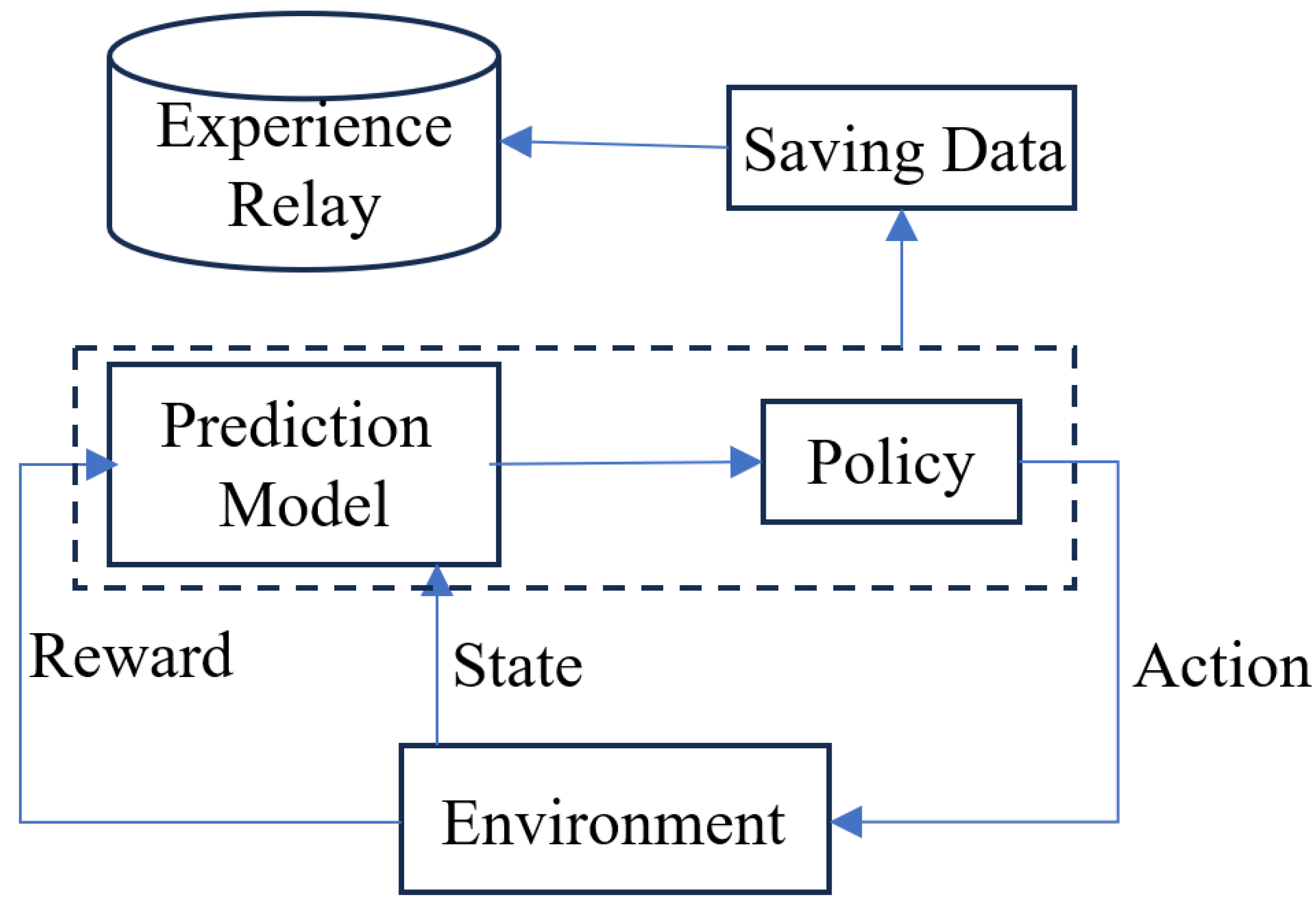
2.5. Deep Q-Network Reinforcement Learning

Reinforcement learning algorithms, in general, are initiated with the help of the Markov Decision Process, which includes a few terms to understand; $O_t$ is an observation, $a_t$ is any action and $r_t$ represents a reward. $s_t$ represents the system state. As the environment learns from itself in this case, $O_t=s_t$. Figure 2 represents the reinforcement learning flowchart; the observation is first obtained from the environment by the agent, which then returns an action to the environment. Based on this action, the environment provides a reward or penalty to the agent in addition to the observation. In the MSL system, the agent action is that of the force applied in moving the UAV to its desired position in the presence of the slung load.

The system state includes the UAV’s position and the slung load pendulum orientation. It is defined as

$$O_t=s_t=\left[{\theta }_x{\dot{\theta }}_x{\theta }_y{\dot{\theta }}_y\right]$$

(72)

The goal for this system is to bring the slung load to the normal position right below the UAV’s centre of mass, such that it has no oscillations. The goal will be achieved when a few conditions pertaining to the vertical position of the pendulum load are within the angular threshold, while the UAV position also remains within the threshold of the XY plane. Initially, the pendulum is placed at a random angle starting position. The episode terminates if the angular threshold is exceeded.

In the course of the interaction, the intelligent agent first determines the next state, $s_{t+1}$, from the environment. In this case, that would be the multirotor’s position and the slung load’s oscillations. Next, it creates an action $a_t$—which in this case is the force applied to move the MSL—based on the current state, and finally earns the reward, $r_{t+1}$, by putting the current action out. The intelligent agent’s ultimate objective is to maximize the cumulative reward over the course of long-term operation, taking into account the benefits acquired during the interaction process.

$$\begin{gathered} g_t=r_{t+1}+\gamma (r_{t+2}+\gamma r_{t+3}+{\gamma }^2{r}_{t+4}+\cdots ) \\ =r_{t+1}+\gamma g_{t+1} \end{gathered}$$

(73)

where $\gamma$ represents the learning rate of the agent.

Reinforcement learning often employs the epsilon greedy method [42] with a Q-table to guide actions based on states. A Q-table is used by the policy to find references representing the relationship between states and actions. Every term in the Q-table represents a Q-value $Q(s_j,a_i)$ where $i=(\mathrm{1,2}\dots m)$ and $j=(\mathrm{1,2}\dots n)$. The chosen action is determined based on the policy of the system in question. However, managing a large Q-table can be cumbersome, especially in complex scenarios like UAV control. To address this, Deep Q-Networks (DQNs) replace the Q-table with neural networks.

In a DQN, one network predicts Q-values (prediction model) and another estimates target Q-values (target model). These networks adjust their weights through gradient descent using the error between target and predicted Q-values. During training, the agent generates training data by interacting with the environment and storing experiences in an experience replay buffer. These experiences are used to update the networks iteratively.

By using neural networks instead of Q-tables, DQN efficiently handles large state–action spaces, making it suitable for complex tasks like UAV control.

In this research, we will utilize the DQN agent to suppress the slung load oscillations, whose flow of control is as expressed in Figure 3. The DQN is used to suppress the pendulum’s oscillations by learning an optimal policy for controlling the pendulum through reinforcement learning. The key idea is to train a neural network to approximate the Q-function, which estimates the expected future rewards for each action given the current state of the system. With the initial environment and system state vector having been defined, a reward function is designed to encourage the pendulum to stay in its normal position, with oscillations suppressed. The reward function is defined as

$$r_t=\left\{\begin{array}{cc}\hfill 1,& \left|\theta \right|\le 1^{\circ }\hfill \\ \hfill -10,& \left|\theta \right|>1^{\circ }\hfill \end{array}\right.$$

(74)

This implies that the DQN agent is rewarded for suppressing the oscillation to within one degree, and penalized tenfold for failing to do so. Hence, the reward function restricts the oscillation angle to $1^{\circ }$, which is further suppressed by the MSSC if necessary.

The network architecture consists of 6 layers; the Feature Input Layer represents the state vector input layer, taking the end effector angle, its velocity, and the UAV position as inputs. The ‘CriticStateFC1’ is a Fully Connected Layer with 24 neurons, while ‘CriticStateFC2’ is another Fully Connected Layer that has 48 neurons. The activation function is a rectified linear unit (ReLU), represented by ‘CriticRelu1’. There is also an additional ReLU layer: the ‘CriticCommonRelu’. A third completely connected layer that has three neurons called ‘Output’ generates the network’s final output. This architecture is summarized in

Table 1. DQN agent layers.

Layer	Name	Definition
1	‘observation’	Feature Input
2	‘CriticStateFC1’	Fully Connected
3	‘CriticStateFC2’	Fully Connected
4	‘CriticRelu1’	Activation Function
5	‘CriticCommonRelu’	ReLU
6	‘Output’	Fully Connected

.

A replay buffer is set up to store present values of the system state, helping to break the correlation between consecutive samples by sampling random mini-batches for training. The MSL must now be trained to have its payload oscillations suppressed. For this, it is provided with training episodes in which the pendulum has various starting positions in each episode. In these episodes, upon obtaining information from the MSL environment, using the epsilon greedy method mentioned above, an action with the highest likelihood of maintaining the maximum reward, based on the selected reward function, is applied to the pendulum, and the resultant oscillation angle and state vector, as well as the reward obtained, are stored in the replay buffer. Periodically, random mini-batches are sampled from this replay buffer, and the target Q-value is calculated using the reward and the highest Q-value from the next state of the target network. The training continues until the desired average reward is maintained, such that the pendulum remains within the predefined threshold regardless of its starting position. The trained policy agent can then be saved and used again without having to re-train a new agent each time that the MSL is required to move from one point to another. Once trained, the DQN agent-based real-time control need not necessarily be trained again unless it is subject to a disturbance of a significantly different nature.

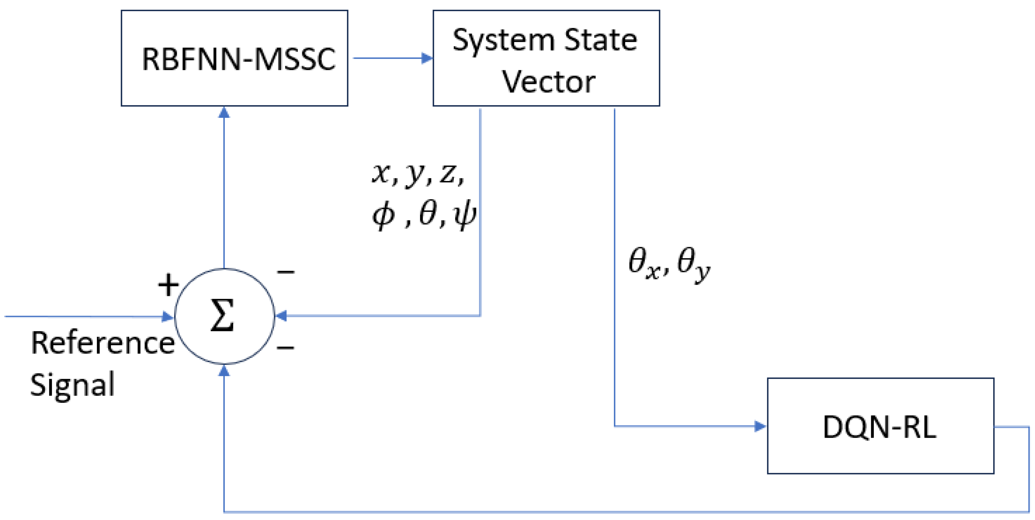
2.6. Control Architecture

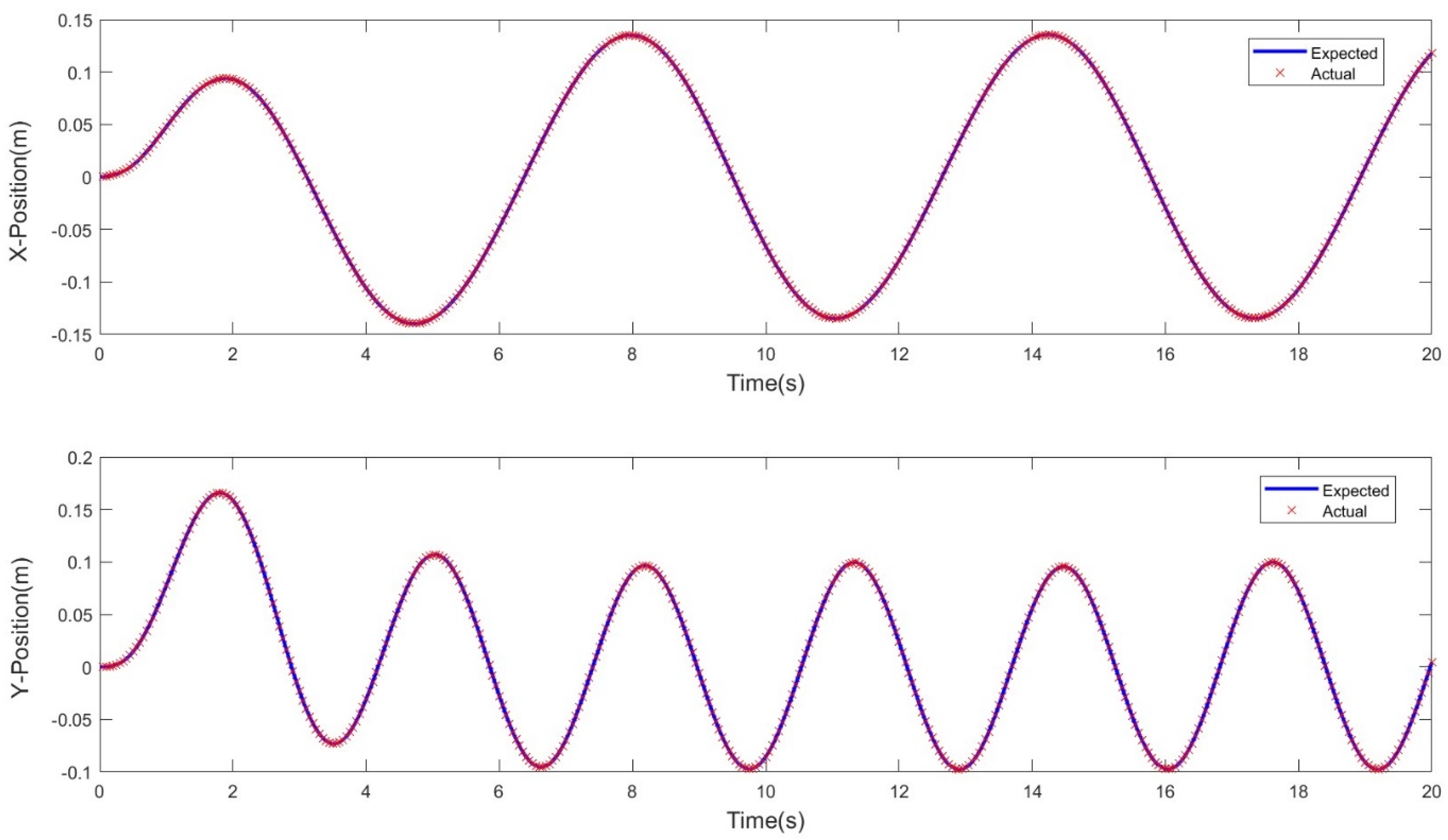
Here, to combine the two controllers, we use the RBFNN-MSSC to maintain the multirotor trajectory and the DQN-RL to train the slung load to suppress its oscillations through self-learning. The architecture of this combined control system is displayed in Figure 4. Initially, the state vector consists of the position and attitude of the multirotor, in addition to the slung load oscillation angles. To feed them into the RBFNN-MSSC, the oscillation angles must be linearized as in (12). These vectors depend upon the magnitude of the oscillation angles. As seen in (72), the DQN agent requires an observation vector, which takes these oscillation angles, ${\theta }_x$ and ${\theta }_y$, as inputs. Once the desired reward as explained in (74) is achieved, the training process is complete. The oscillation angles have been suppressed to a certain limit and can then be fed back into the system control loop. The RBFNN-MSSC then ensures that the desired trajectory of the system is achieved, by minimizing the error from the reference signal, which indicates the ideal trajectory of the multirotor and the desired orientation of the slung load.

3. Results

To verify the effectiveness of the proposed control, we have implemented some simulations in MATLAB R2022b. The parameters for the simulation are defined in

Table 2. Simulation parameters.

Parameters	Symbols	Values
Multirotor mass	M	4 kg
Slung load mass	m	0.5 kg
Slung load link length	l	1 m
Rotor speed for hover	ωres	29,700 m/s
UAV moment of inertia	I	2.07 × 10−2 kg/m2
Feedback control time step	Tc	0.005
Simulation run time	T	10 s
Sampling rate	Ts	0.01 s
Learning rate	γ	5 × 10−3

. The sliding surface ratios are taken as 0.8, 1.0 and 1000 for $s_1$, $s_2$, and $s_3$, respectively. We train the system which is subject to an initial disturbance with a vector defined by $0.6\times rand\left(n\right)+0.1$, where $rand\left(n\right)$ generates a number between 0 and 1.

The training of the DQN agent yields the results as seen in Figure 5. Each episode is implemented for 500 steps, and would terminate if the threshold of $1^{\circ }$ is exceeded upon entering into the bounds of $[-1^{\circ },1^{\circ }]$. Upon achieving the desired reward, the agent could be saved and used for future simulations, i.e., it need not be trained each time a simulation is implemented. The resultant oscillation angle is then fed back into the MSSC control loop. To verify its effectiveness, we compare its performance with the MSSC being applied to the slung load as part of the MSL as well, in contrast to it being controlled by the RL agent.

The parameters used for the simulation are highlighted in Table 2. We first consider the case of the MSL control along a square path. The robustness of the trajectory tracking is highlighted in Figure 6, where the sliding surfaces ensure that the quadrotor remains within the bounds of the desired path. In tracking this square trajectory, there is a slight offset from the desired path each time that a turn is performed at the corner of the desired square path, as seen in Figure 7, but it is quickly able to get back on track along the linear path of movement. The magnitude of reduction in slung load oscillations is greater with the RL agent over the MSSC, as represented in Figure 8, with a lower peak and a slightly quicker convergence. In Figure 9, the control inputs indicate that the initial chattering effect brought about by the disturbances applied to the MSL is quickly suppressed by the RBFNN. Hence, the proposed control architecture is effective when the MSL traces a square path.

To further validate the proposed control, we next consider a butterfly path. Once again, the sliding surfaces represented in Figure 10 indicate that the MSL is kept within the bounds of the desired path, whose tracked trajectory is shown in Figure 11. The step response characteristics displayed in

Table 3. Step response characteristics of MSSC vs. RL.

Parameter	Value
	Butterfly Trajectory		Square Trajectory
	MSSC	RL	MSSC	RL
Rise time	0.01	0.006	0.008	0.006
Transient time	27.08	22.6	25.35	22.21
Settling time	29.94	29.98	29.98	29.97
Settling min	−0.12	−0.12	−2.55	−3.26
Settling max	1.43	1.01	3.53	2.91
Overshoot	2.71	6.94	3.81	4.0
Undershoot	3.6	1.1	4.04	3.58
Peak	1.83	1.58	3.75	3.26
Peak time	1.01	0.37	1.02	0.38

highlight the reduction in the transient time of the slung load pendulum when utilizing the DQN-based RL over the RBFNN-MSSC. A reduction in the undershoot represents a reduction in the lag of the pendulum behind the forward-moving trajectory of the multirotor. The peak is reduced by about 20%, while the peak time is also significantly reduced by 66%. The trajectory traced here is almost point for point, even in the presence of applied impulse disturbances. The effectiveness of the DQN-RL agent over the RBFNN-MSSC on its own is once again displayed in Figure 12, where the oscillation of the slung load is reduced. This reduction is further emphasized in

Table 4. Quantitative data of slung load oscillations.

Parameter		Max	Mean	RMS
Butterfly Trajectory	MSSC	1.43	−0.01	0.37
	RL	1.01	−0.01	0.26
Square Trajectory	MSSC	3.53	−1.22 × 10−4	0.98
	RL	2.92	−7.41 × 10−4	0.70

, where we see that the oscillation angle, in utilizing the RL agent over the MSSC, is reduced by 30%. Finally, Figure 13 displays the elimination of the chattering effect even when there is a change in direction at every instant, with the addition of the RBFNN to the MSSC.

4. Conclusions

In this paper, we proposed a robust adaptive controller in which a Multi-Surface Sliding Mode Controller was aided by a Radial Basis Function Neural Network to ensure that a multirotor carrying a suspended payload would have a guaranteed asymptotic stability within certain bounds. To suppress the oscillations of the suspended payload, we combined the RBFNN-MSSC with a Deep Q-Network-based reinforcement learning agent, with a reward function that would focus on limiting the oscillations to a certain threshold. Upon comparing the results of this control architecture with a control system employing the RBFNN-MSSC on its own for the entire system, based on the oscillations of the suspended payload, the proposed architecture was found to be the more effective of the two. Lyapunov Stability Theory was also proposed to verify the effectiveness of the proposed control. Future work may include proposing an additional reward function for the multirotor to combine with that proposed for the suspended payload.

References

1. Nawaz, H.; Ali, H.M.; Massan, S. Applications of unmanned aerial vehicles: A review. Tecnol. Glosas Innovación Apl. Pyme. Spec. 2019, 2019, 85–105. [Google Scholar] [CrossRef]
2. Emran, B.J.; Najjaran, H. A review of quadrotor: An underactuated mechanical system. Annu. Rev. Control. 2018, 46, 165–180. [Google Scholar] [CrossRef]
3. Baraean, A.; Hamanah, W.M.; Bawazir, A.; Quama, M.M.; El Ferik, S.; Baraean, S.; Abido, M.A. Optimal Nonlinear backstepping controller design of a Quadrotor-Slung load system using particle Swarm Optimization. Alex. Eng. J. 2023, 68, 551–560. [Google Scholar] [CrossRef]
4. Al-Dhaifallah, M.; Al-Qahtani, F.M.; Elferik, S.; Saif, A.-W.A. Quadrotor robust fractional-order sliding mode control in unmanned aerial vehicles for eliminating external disturbances. Aerospace 2023, 10, 665. [Google Scholar] [CrossRef]
5. Manalathody, A.; Krishnan, K.S.; Subramanian, J.A.; Thangavel, S.; Thangeswaran, R.S.K. Non-linear Controller for a Drone with Slung Load. In Proceedings of the International Conference on Modern Research in Aerospace Engineering, Noida, India, 21–22 September 2023; pp. 219–228. [Google Scholar]
6. Li, B.; Li, Y.; Yang, P.; Zhu, X. Adaptive neural network-based fault-tolerant control for quadrotor-slung-load system under marine scene. IEEE Trans. Intell. Veh. 2023, 9, 681–691. [Google Scholar] [CrossRef]
7. Wang, Z.; Qi, J.; Wu, C.; Wang, M.; Ping, Y.; Xin, J. Control of quadrotor slung load system based on double ADRC. In Proceedings of the 2020 39th Chinese Control Conference (CCC), Shenyang, China, 27–29 July 2020; pp. 6810–6815. [Google Scholar]
8. Ren, Y.; Zhao, Z.; Ahn, C.K.; Li, H.-X. Adaptive fuzzy control for an uncertain axially moving slung-load cable system of a hovering helicopter with actuator fault. IEEE Trans. Fuzzy Syst. 2022, 30, 4915–4925. [Google Scholar] [CrossRef]
9. Gajbhiye, S.; Cabecinhas, D.; Silvestre, C.; Cunha, R. Geometric finite-time inner-outer loop trajectory tracking control strategy for quadrotor slung-load transportation. Nonlinear Dyn. 2022, 107, 2291–2308. [Google Scholar] [CrossRef]
10. Tolba, M.; Shirinzadeh, B.; El-Bayoumi, G.; Mohamady, O. Adaptive optimal controller design for an unbalanced UAV with slung load. Auton. Robot. 2023, 47, 267–280. [Google Scholar] [CrossRef]
11. Wang, Y.; Yu, G.; Xie, W.; Zhang, W.; Silvestre, C. UDE-based Robust Control of a Quadrotor-Slung-Load System. IEEE Robot. Autom. Lett. 2023, 8, 6851–6858. [Google Scholar] [CrossRef]
12. Kabzan, J.; Hewing, L.; Liniger, A.; Zeilinger, M.N. Learning-based model predictive control for autonomous racing. IEEE Robot. Autom. Lett. 2019, 4, 3363–3370. [Google Scholar] [CrossRef]
13. Bag, A.; Subudhi, B.; Ray, P.K. A combined reinforcement learning and sliding mode control scheme for grid integration of a PV system. CSEE J. Power Energy Syst. 2019, 5, 498–506. [Google Scholar]
14. Lee, D.; Lee, S.J.; Yim, S.C. Reinforcement learning-based adaptive PID controller for DPS. Ocean Eng. 2020, 216, 108053. [Google Scholar] [CrossRef]
15. Rizvi, S.A.A.; Lin, Z. Reinforcement learning-based linear quadratic regulation of continuous-time systems using dynamic output feedback. IEEE Trans. Cybern. 2019, 50, 4670–4679. [Google Scholar] [CrossRef] [PubMed]
16. Annaswamy, A.M. Adaptive control and intersections with reinforcement learning. Annu. Rev. Control Robot. Auton. Syst. 2023, 6, 65–93. [Google Scholar] [CrossRef]
17. Du, B.; Lin, B.; Zhang, C.; Dong, B.; Zhang, W. Safe deep reinforcement learning-based adaptive control for USV interception mission. Ocean Eng. 2022, 246, 110477. [Google Scholar] [CrossRef]
18. Wu, L.; Wang, C.; Zhang, P.; Wei, C. Deep reinforcement learning with corrective feedback for autonomous uav landing on a mobile platform. Drones 2022, 6, 238. [Google Scholar] [CrossRef]
19. Liang, X.; Du, X.; Wang, G.; Han, Z. Deep reinforcement learning for traffic light control in vehicular networks. arXiv 2018, arXiv:1803.11115. [Google Scholar]
20. Ma, S.; Lee, J.; Serban, N.; Yang, S. Deep Attention Q-Network for Personalized Treatment Recommendation. In Proceedings of the 2023 IEEE International Conference on Data Mining Workshops (ICDMW), Shanghai, China, 4 December 2023; IEEE: Piscataway, NJ, USA; pp. 329–337. [Google Scholar]
21. Peng, B.; Sun, Q.; Li, S.E.; Kum, D.; Yin, Y.; Wei, J.; Gu, T. End-to-end autonomous driving through dueling double deep Q-network. Automot. Innov. 2021, 4, 328–337. [Google Scholar] [CrossRef]
22. Fang, X.; Gong, G.; Li, G.; Chun, L.; Peng, P.; Li, W.; Shi, X.; Chen, X. Deep reinforcement learning optimal control strategy for temperature setpoint real-time reset in multi-zone building HVAC system. Appl. Therm. Eng. 2022, 212, 118552. [Google Scholar] [CrossRef]
23. Kersandt, K.; Muñoz, G.; Barrado, C. Self-training by reinforcement learning for full-autonomous drones of the future. In Proceedings of the 2018 IEEE/AIAA 37th Digital Avionics Systems Conference (DASC), London, UK, 23–27 September 2018; pp. 1–10. [Google Scholar]
24. Muñoz, G.; Barrado, C.; Çetin, E.; Salami, E. Deep reinforcement learning for drone delivery. Drones 2019, 3, 72. [Google Scholar] [CrossRef]
25. Raja, G.; Baskar, Y.; Dhanasekaran, P.; Nawaz, R.; Yu, K. An efficient formation control mechanism for multi-UAV navigation in remote surveillance. In Proceedings of the 2021 IEEE Globecom Workshops (GC Wkshps), Madrid, Spain, 7–11 December 2021; pp. 1–6. [Google Scholar]
26. Özalp, R.; Varol, N.K.; Taşci, B.; Uçar, A. A review of deep reinforcement learning algorithms and comparative results on inverted pendulum system. In Machine Learning Paradigms. Learning and Analytics in Intelligent Systems; Springer: Cham, Switzerland, 2020; pp. 237–256. [Google Scholar]
27. Dang, K.N.; Van, L.V. Development of deep reinforcement learning for inverted pendulum. Int. J. Electr. Comput. Eng. 2023, 13, 3895–3902. [Google Scholar]
28. Li, X.; Liu, H.; Wang, X. Solve the inverted pendulum problem base on DQN algorithm. In Proceedings of the 2019 Chinese Control and Decision Conference (CCDC), Nanchang, China, 3–5 June 2019; pp. 5115–5120. [Google Scholar]
29. Huang, H.; Yang, Y.; Wang, H.; Ding, Z.; Sari, H.; Adachi, F. Deep reinforcement learning for UAV navigation through massive MIMO technique. IEEE Trans. Veh. Technol. 2019, 69, 1117–1121. [Google Scholar] [CrossRef]
30. Wang, S.; Qi, N.; Jiang, H.; Xiao, M.; Liu, H.; Jia, L.; Zhao, D. Trajectory Planning for UAV-Assisted Data Collection in IoT Network: A Double Deep Q Network Approach. Electronics 2024, 13, 1592. [Google Scholar] [CrossRef]
31. Hedrick, J.K.; Yip, P.P. Multiple sliding surface control: Theory and application. J. Dyn. Sys. Meas. Control 2000, 122, 586–593. [Google Scholar] [CrossRef]
32. Thanh, H.L.N.N.; Hong, S.K. An extended multi-surface sliding control for matched/mismatched uncertain nonlinear systems through a lumped disturbance estimator. IEEE Access 2020, 8, 91468–91475. [Google Scholar] [CrossRef]
33. Ullah, S.; Khan, Q.; Mehmood, A.; Bhatti, A.I. Robust backstepping sliding mode control design for a class of underactuated electro–mechanical nonlinear systems. J. Electr. Eng. Technol. 2020, 15, 1821–1828. [Google Scholar] [CrossRef]
34. Qu, X.; Zeng, Z.; Wang, K.; Wang, S. Replacing urban trucks via ground–air cooperation. Commun. Transp. Res. 2022, 2, 100080. [Google Scholar] [CrossRef]
35. Nyaaba, A.A.; Ayamga, M. Intricacies of medical drones in healthcare delivery: Implications for Africa. Technol. Soc. 2021, 66, 101624. [Google Scholar] [CrossRef]
36. Rejeb, A.; Abdollahi, A.; Rejeb, K.; Treiblmaier, H. Drones in agriculture: A review and bibliometric analysis. Comput. Electron. Agric. 2022, 198, 107017. [Google Scholar] [CrossRef]
37. Zheng, C.; Yan, Y.; Liu, Y. Prospects of eVTOL and modular flying cars in China urban settings. J. Intell. Connect. Veh. 2023, 6, 187–189. [Google Scholar] [CrossRef]
38. Khoo, S.; Norton, M.; Kumar, J.J.; Yin, J.; Yu, X.; Macpherson, T.; Dowling, D.; Kouzani, A. Robust control of novel thrust vectored 3D printed multicopter. In Proceedings of the 2017 36th Chinese Control Conference (CCC), Dalian, China, 26–28 July 2017; pp. 1270–1275. [Google Scholar]
39. Peris, C.; Norton, M.; Khoo, S.Y. Variations in Finite-Time Multi-Surface Sliding Mode Control for Multirotor Unmanned Aerial Vehicle Payload Delivery with Pendulum Swinging Effects. Machines 2023, 11, 899. [Google Scholar] [CrossRef]
40. Peris, C.; Norton, M.; Khoo, S.Y. Multi-surface Sliding Mode Control of a Thrust Vectored Quadcopter with a Suspended Double Pendulum Weight. In Proceedings of the IECON 2021–47th Annual Conference of the IEEE Industrial Electronics Society, Toronto, ON, Canada, 13–16 October 2021; pp. 1–6. [Google Scholar]
41. Clevon Peris, M.N.; Khoo, S.Y. Adaptive Multi Surface Sliding Mode Control of a Quadrotor Slung Load System. In Proceedings of the IEEE 10th International Conference on Automation, Robotics and Application (ICARA 2024), Athens, Greece, 23 February 2024. [Google Scholar]
42. Kuang, N.L.; Leung, C.H. Performance effectiveness of multimedia information search using the epsilon-greedy algorithm. In Proceedings of the 2019 18th IEEE International Conference on Machine Learning and Applications (ICMLA), Boca Raton, FL, USA, 16–19 December 2019; pp. 929–936. [Google Scholar]
Figure 1. Model of a quadcopter with a suspended pendulum load.
Electronics 13 02424 g001
Figure 2. General flow of an RL control system.
Electronics 13 02424 g002
Figure 3. RL using the DQN method.
Electronics 13 02424 g003
Figure 4. Framework of the RBFNNMSSC with DQN-RL.
Electronics 13 02424 g004
Figure 5. Training of the DQN agent for real-time control of the slung load.
Electronics 13 02424 g005
Figure 6. Sliding surfaces for trajectory tracking along a square path.
Electronics 13 02424 g006
Figure 7. Trajectory tracking of the multirotor by the RBFNN-MSSC.
Electronics 13 02424 g007
Figure 8. Comparison of the slung load oscillation with MSSC and with RL along a square path.
Electronics 13 02424 g008
Figure 9. Control inputs (rotor tilt angles) along the square path.
Electronics 13 02424 g009
Figure 10. Sliding surfaces for trajectory tracking along a butterfly path.
Electronics 13 02424 g010
Figure 11. Trajectory tracking of the multirotor by the RBFNN-MSSC along a butterfly path.
Electronics 13 02424 g011
Figure 12. Comparison of the slung load oscillation with MSSC and with RL along the butterfly path.
Electronics 13 02424 g012
Figure 13. Control inputs (rotor tilt angles) along the butterfly path.
Electronics 13 02424 g013