Abstract
The welding quality during welding body-in-white (BIW) determines the safety of automobiles. Due to the limitations of testing cost and cycle time, the prediction of welding quality has become an essential safety issue in the process of automobile production. Conventional prediction methods mainly consider the welding process parameters and ignore the material parameters, causing their results to be unrealistic. Upon identifying significant correlations between vehicle body materials, we utilize principal component analysis (PCA) to perform dimensionality reduction and extract the underlying principal components. Thereafter, we employ a greedy feature selection strategy to identify the most salient features. In this study, a welding quality prediction model integrating process parameters and material characteristics is proposed, following which the influence of material properties is analyzed. The model is verified based on actual production data, and the results show that the accuracy of the model is improved through integrating the production process characteristics and material characteristics. Moreover, the overfitting phenomenon can be effectively avoided in the prediction process.
1. Introduction
In many industries, such as automobile production, aerospace vehicles, and ships, resistance spot-welding (RSW) is one of the most widely used material connection methods [1]. RSW is a comprehensive process integrating mechanical, electrical, thermal metallurgy, and other knowledge fields. Solder joint forming is a highly coupled non-linear process with multiple interacting factors [2]. It is difficult to directly establish a single mathematical mapping relationship between the production process and welding quality.
With the emergence of personalized needs and the utilization of new materials, it has been found that different combinations with the same material properties also lead to great differences in welding quality, and that the combination mode of materials also has a great impact on welding. At the same time, welding is the result of multi-factor fusion and the effects of these factors change under different constraints. Therefore, the welding quality of new material combinations is required to be predicted rapidly and the process parameters should be evaluated within a short time.
Vignesh et al. [3] adopted the finite element analysis method of mathematical approximation to simulate and compare the real tensile and shear experiments using simulation software to study the fracture of solder joints. This method can predict the nugget formation process under different welding conditions, but the multi-physical processes of resistance spot-welding cannot be fully taken into account. Bae et al. [4] predicted and analyzed the tensile shear load of heterogeneous metals with the response surface method (RSM) to obtain a more appropriate combination of welding parameters. Although the response surface method can establish the quadratic polynomial correlation model between welding parameters and quality indices, the highly non-linear process is not considered in this method and the end result is often only locally optimal.
With the development of machine learning technology, an important research direction has been explored, involving the use of data mining technology to analyze existing data and determine the relationships between process, material, and quality. To date, a lot of relevant research work has been carried out. For example, Zhao et al. [2] put forward an optimization method for spot-welding parameters based on regression analysis and weight entropy. In this method, quality indices including tensile shear load and nugget diameter are assigned weights and integrated into a comprehensive quality index using the Gray entropy method, and a quantitative mathematical model between process parameters and comprehensive indexes was obtained. This numerical method can provide empirical guidance for the same welding material combination, but cannot be transferred to handle different new material combinations, which will lead to slow product manufacturing and delivery in practical application.
Vigneshkumar and Varthanan [5] took control parameters such as welding current, electrode pressure, welding time, and penetration depth as the input of and artificial neural network (ANN) and the tensile shear strength of the nugget as the output. Hoseini et al. [6] studied the relationship between the shear tensile strength of an alloy nugget and process parameters using an ANN. Chen et al. [7] analyzed welding process data by Gray correlation analysis and principal component analysis, and constructed a back propagation neural network model combined with genetic algorithm to predict the important characteristics of spot-welding. Gavidel et al. [8] computed the sampling distribution for each prediction model through bootstrapping, then designed a ANN for non-destructive nugget width estimation and, finally, accurately predicted the welding quality under variable welding parameters. Lee et al. [9] introduced novel deep learning autoencoder models to enhance production efficiency through presenting a comparative assessment for anomaly detection, enabling precise and predictive insights through modeling complex temporal relationships in the vibration data. However, ANNs are prone to falling into the situation of overfitting when dealing with small data sets. In order to solve this problem, more manual attempts are needed to design the network structure and train the model to obtain complex hyperparameters. Moreover, the selection of network hyperparameters lacks adequate explanation.
At present, the research directions can be mainly divided into forward simulation based on physical characteristics and quality prediction based on data mining. The former mainly studies the nugget formation mechanism through mechanical and thermal analyses, and establishes a physical model to predict the welding quality. The latter, through employing data mining technology, analyzes the mathematical mapping relationship between welding quality and influencing factors in the existing welding process information data in order to achieve the objectives of optimizing welding parameters and predicting welding quality. To date, the latter research has mainly analyzed the direct mapping relationship between process parameters and welding quality, with a focus on process factors such as the welding current, pressure, and time.
However, in fact, the mechanical and physical properties and chemical composition content of different materials constitute the most important factors determining the nugget performance. In this study, first, the material name data in the original data are converted into material chemical composition and physical properties to acquire new data set. Second, the characteristics of materials and welding process parameters are integrated as the input part of the training model. The chemical composition and properties of materials are paramount to their performance, whereas the material characteristics exhibit inherent redundancy, as evidenced by high pairwise correlations (e.g., Pearson correlation coefficients exceeding 0.9). To mitigate this issue, we utilized principal component analysis (PCA) to transform the material features, preserving approximately 90% of the variance, and derive the principal component features. Thereafter, we apply a greedy feature selection strategy to identify the most salient features. Third, the optimal feature combination is determined by virtue of a variety of methods. Then, the Bayesian optimization method is applied and the prediction model is constructed. In the obtained model, the reasonable process parameters are then analyzed using particle swarm optimization algorithm, and can be used as a reference for welding design and welding parameter design.
2. Methodology
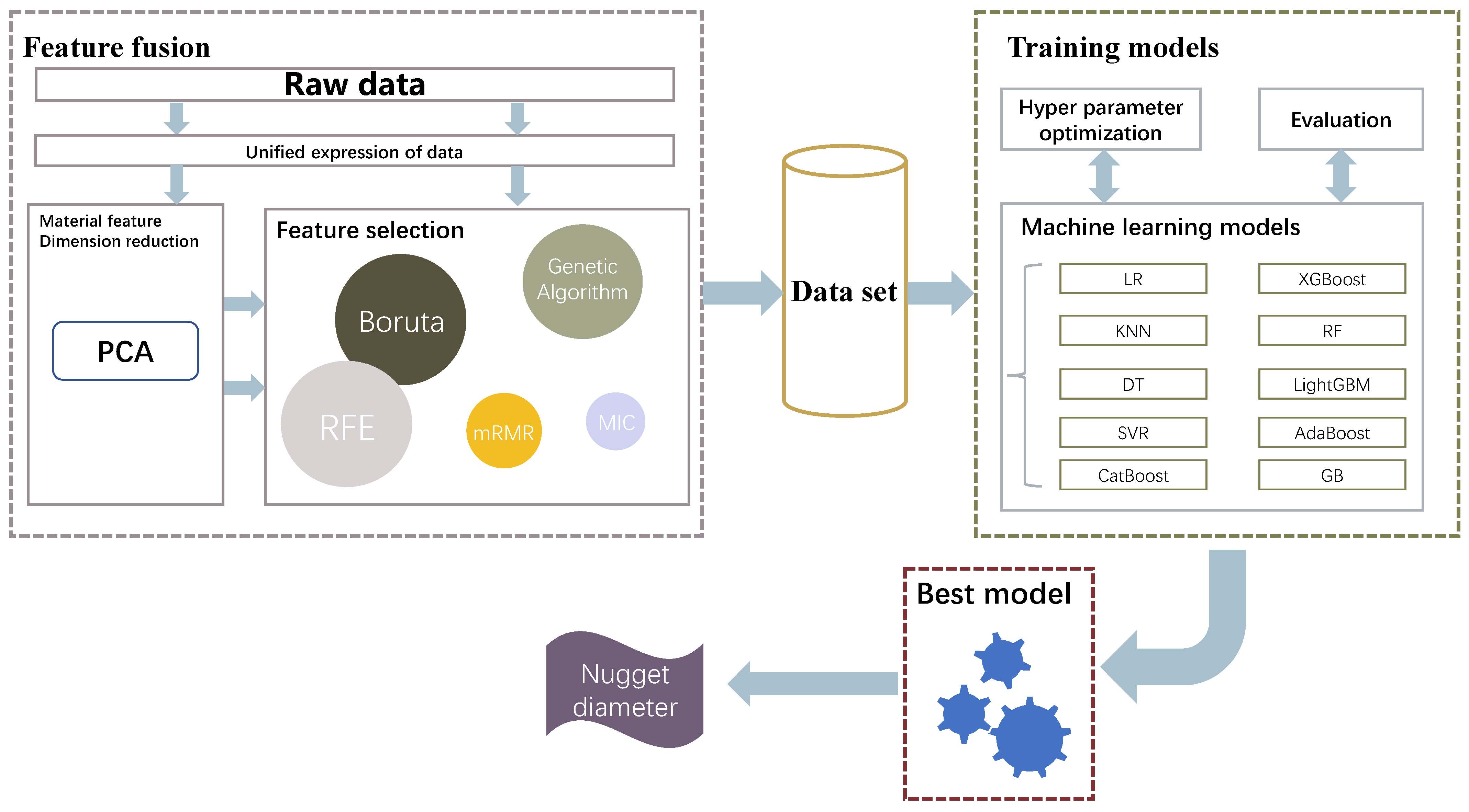
The overall algorithm framework is shown in Figure 1.

Figure 1.
Overall framework of data mining algorithm.
2.1. Data Preprocess
In this paper, the analyzed body-in-white (BIW) welding information mainly includes process data and material data. As shown in Table 1, the process data mainly refer to digital data such as the welding current, welding time, electrode pressure, and electrode diameter. Combined with the actual production situation, this study splits the characteristic information of the original material to obtain the thickness, coating, material, and other information. The welding data were obtained from a resistance spot welding experiment using heterogeneous three-layer plates with unequal thickness.

Table 1.
Characteristic parameters.
Furthermore, this study converts the characteristics of welding materials into chemical composition and mechanical properties. Chemical composition parameters include the carbon (C) concentration, manganese (Mn) concentration, phosphorus (P) concentration, sulfur (S) concentration, and total aluminum content (alt), alongside physical properties comprising yield strength, tensile strength, elongation, strain hardening exponent (N), plastic strain ratio (R), and thickness.
Various characteristics, such as welding current, electrode pressure, electrode diameter, material properties, and process expression, vary greatly and have different orders of magnitude. Therefore, if the original data are directly used as an input, the stability and accuracy of the model will be greatly affected. The standardized processing of the input characteristic variable data can yield better results. In this study, the standardized method is considered for data processing. According to our test results, the Z-score method [10] is used to normalize the data, achieving a good application effect.
2.2. The Design of Dimensionality Reduction Algorithm Based on PCA
In the actual production process, it is impossible to detect the welding quality simply by vigorously destroying products. Therefore, tear resistance cannot be deemed as the evaluation standard of welding quality. According to practical operation experience, the performance of the welding quality is most directly related to the diameter and shape of the weld nugget. Combining with theory [11], the study selects the nugget diameter as one of the evaluation criteria for welding quality.
After the data set was preprocessed, more than 40 influencing factors were summarized. In order to simplify the model and improve the calculation efficiency, dimensionality reduction processing was performed on the original data set to determine these important influencing factors. PCA is a method for reducing the dimensionality of data while retaining the overall information [12]. In view of the actual processing situation, combined with the data characteristics, the dimensionality reduction algorithm based on PCA used in this study is as follows:
- In the original data class, the whole influencing factors are divided into two categories: a process parameter set and a material parameter set . Then, a set of mutually orthogonal coordinate axes are found in the corresponding data space, and the variables are projected onto these coordinate axes.
- The covariance difference is chosen to represent the distance between variables. The larger the covariance, the more information will be retained. Therefore, one group of m-dimensional original variables can be transformed into a group of -dimensional unrelated main variables.
- The covariance between and iswhere and are the mean of random variables, and is the element of vector . Then, the covariance matrix C of material can be calculated asThe pair covariance matrix is decomposed as:The eigenvalues of the covariance matrix are calculated as (arranged in descending order) and the corresponding unitized eigenvector . is the mth component of the jth eigenvector.where refers to the ith principal component. The contribution rate of the principal component is and the cumulative contribution rate is expressed by :
- The selection of principal components is determined according to several thresholds. In this study, two thresholds are chosen: the eigenvalue is greater than 1 and the cumulative contribution rate reaches 90%. Through many tests, this should guarantee that the selected main components can not only retain the original and complete amount of information, but also can reduce the required number of calculations, which can efficiently improve the performance of the model. For example, the main components and components selected for material characteristic parameters are recorded as
- After the above processing, three types of training data sets are obtained. The first type is the training set containing only process parameters:The second type is the training set of process parameters and material parameters:The third type is the training set for PCA fusion of process parameters and material parameters:
2.3. Feature Selection Methods
Although the dimensionality reduction processing was carried out for influencing factors, it is necessary to further determine the most important and influential features.
Considering that these factors involve many aspects, they cannot be simply extracted empirically. Therefore, combined with data features, minimal redundancy maximal relevance (MRMR) was selected to analyze the function of features from different perspectives. Finally, the unified expression was utilized to obtain the optimal feature combination.
MIC has the ability to capture the non-functional mapping relationship between the two variables and is not affected by the specific form of relationship to produce deviation [13].
The core idea of the MRMR is to maximize the correlation between features and target variables and minimize the correlation between each feature [14]. In this study, there exists a certain degree of redundant information overlap between internal features. For example, with respect to the aforementioned materials, a certain correlation was found between the chemical attribute Ca content and the physical attribute of shear force.
The Boruta feature selection method [15] is a packaging algorithm based on random forest. In this study, a random forest classifier is added into the input data set to select the optimal features according to the index ranking, following which the feature selection set is obtained by means of model construction.
The RFE algorithm is based on the idea of greed, which mainly selects the current optimal variable during iterative model construction, then deletes the selected variables and continues to repeat until all remaining variables are traversed [16]. In this study, linear regression, ridge regression, and other methods were tested. Finally, the random forest algorithm was selected as the classifier of the RFE model.
A Genetic algorithm is a heuristic global search method, aiming at solving both constrained and unconstrained optimization problems based on the principles of natural selection.
Using the above five models, the feature set X of each model was obtained. Finally, the multi-dimensional optimal feature combination set can be expressed as
where X is the training feature set and is the weight matrix.
is the data set, which should be used as input to the machine learning model in the next step for calculation.
2.4. Multi-Model Machine Learning Algorithm Based on Bayesian
- Basic model selectionIn this study, two types of algorithms were selected as basic models: linear methods and integrated learning methods. The first type of basic model mainly includes multi-linear regression, k-nearest neighbor, and support vector machine regression (SVR) models. The second type mainly covers XGBoost, LightGBM, and CatBoost. SVR has strong fitting ability for data sets with small amounts of data. Extreme gradient enhancement (XGBoost) is an integrated machine learning model. LightGBM is an efficient gradient-lifting decision tree algorithm proposed by Microsoft. CatBoost is also an algorithm based on decision tree, with a low number of parameters and support for categorical variables.
- Model fusion and implementationIn practical application, it has been demonstrated many times that the general result of simply using the above algorithms leads to two extreme phenomena:
- (a)
- The effect is good in the modeling data set, but it is difficult to achieve the ideal effect in the test data set.
- (b)
- The machine learning algorithm lacks sufficient capacity to capture the underlying patterns and relationships in the data, resulting in poor performance.
During basic model training, the minimum variance and deviation are computed. Specifically, the variance is calculated according to the prediction data of the test set, and the deviation is calculated in accordance with the error of the training data. In order to avoid the overfitting phenomenon, this study combines the Bayesian optimization algorithm [17] to complete the parameter selection of the basic model, thus improving the model performance and reducing variance. Therefore, this study proposes a machine learning synthesis model based on Bayesian optimization:where x represents the hyperparameter to be optimized in the machine learning model, X represents the search space of super parameters, and denotes the objective function l, that is, the black-box model that inputs a set of hyperparameters and outputs the evaluation indices.In order to obtain the optimal x, the Bayesian optimization algorithm is further used to iteratively calculate the sampling function . is the objective function value of the current optimal x, and are the mean and variance of the objective function obtained by the Gaussian process—that is, the posterior distribution of —and is the trade-off coefficient to prevent obtaining the local optimal solution of . The implementation procedure of the Bayesian iterative optimization algorithm is given as Algorithm 1.Algorithm 1 Bayesian iterative optimization algorithm - 1:
- Input: , number of iterations T.
- 2:
- Calculate
- 3:
- for 1 to T do
- 4:
- 5:
- 6:
- 7:
- Rebuild Gaussian process model and calculate
- 8:
- end for
- 9:
- Output: X
- Model performance index selectionRegarding the utilization of machine learning to solve practical production problems, it is essential to select an evaluation index for model quality. This study uses several quantitative indicators to measure the uncertainty between measurement and calculation results in order to evaluate the model performance from different perspectives. These various quantitative indicators are defined as follows:where reflects the fitting accuracy of the model to the data. and take non-negative values. represents the proportion of data that can be interpreted by the data model. The average absolute relative deviation is used to judge the evaluation accuracy. denotes the percentage of accuracy and precision, which indicates the reliability of a model.
3. Experiments and Analysis
3.1. Data Sources
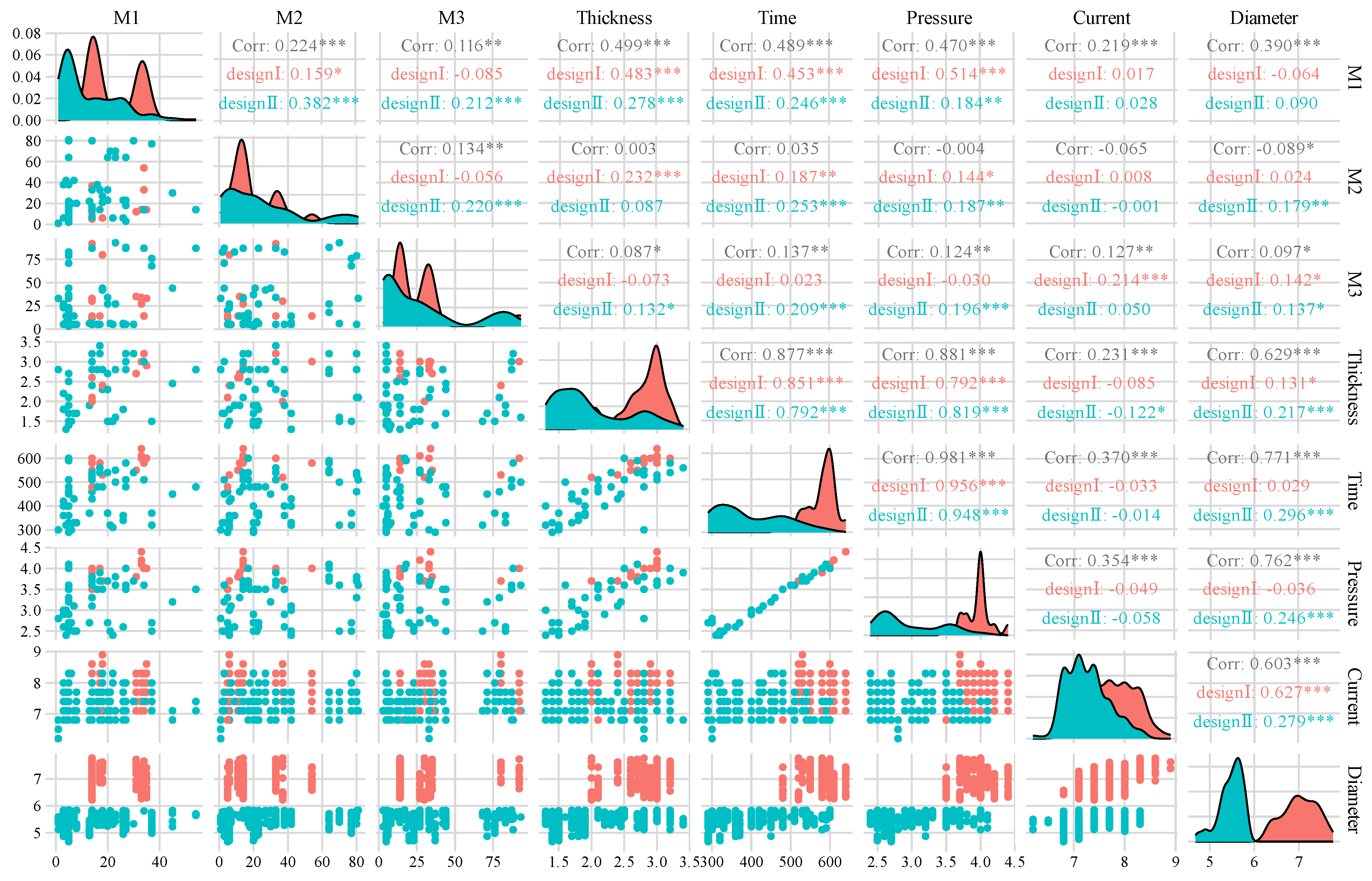
The data set used in this study comes from the experimental results of the lap resistance spot-welding of three-layer heterogeneous plates in the laboratory. The input characteristics of the data set are divided into design parameters, process parameters, and material parameters. Design parameters include design diameter, thickness, material type, and so on. Process parameters comprise welding current, welding time, electrode pressure, electrode diameter, and so on. Material parameters include mechanical property parameters, chemical element contents, quality parameters, and nugget diameter (see Table 1 for details). The three-layer plate welding combination of the key parts of the automobile body-in-white was selected to carry out the lap spot-welding experiment. The design diameter was divided into a cm and b cm. When the actual measured nugget diameter is greater than the design value, the vehicle body performance and safety indicators are satisfied. The variable distribution and correlation of the input design parameters and process parameters are shown in Figure 2. The different significance levels in the statistical results are indicated by p-values, where * denotes p < 0.05, ** denotes p < 0.01, and *** denotes p < 0.001. The mechanical properties of the alloy welding materials, including yield strength, tensile strength, and elongation, not only depend on the fiber structure state and production process parameters, but also the chemical composition, which exerts an important impact on the performance indices [18].
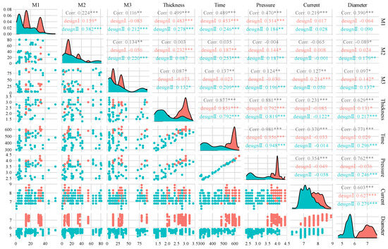
Figure 2.
Data characteristic distribution map.
In order to deal with the design characteristics of different parts of the automobile body, it is significant to design and produce different materials with different thicknesses. Through calculating the Pearson correlation coefficients of these material characteristics, it was found that there exist strong correlations between some characteristics. From the heatmap of correlation between material characteristics shown in Figure 3, across three disparate material categories, a pronounced correlation was observed between elongation and various mechanical properties, including P, S, alt, yield strength, and tensile strength. Specifically, the heatmap visualizations revealed intense coloration for the pairwise relationships between elongation and P, elongation and S, elongation and tensile strength, and elongation and yield strength, revealing linear correlations between these pairs of characteristics.

Figure 3.
Thermodynamic diagram of Pearson coefficients between material mechanical properties and chemical element contents. (a) Material 1. (b) Material 2. (c) Material 3.
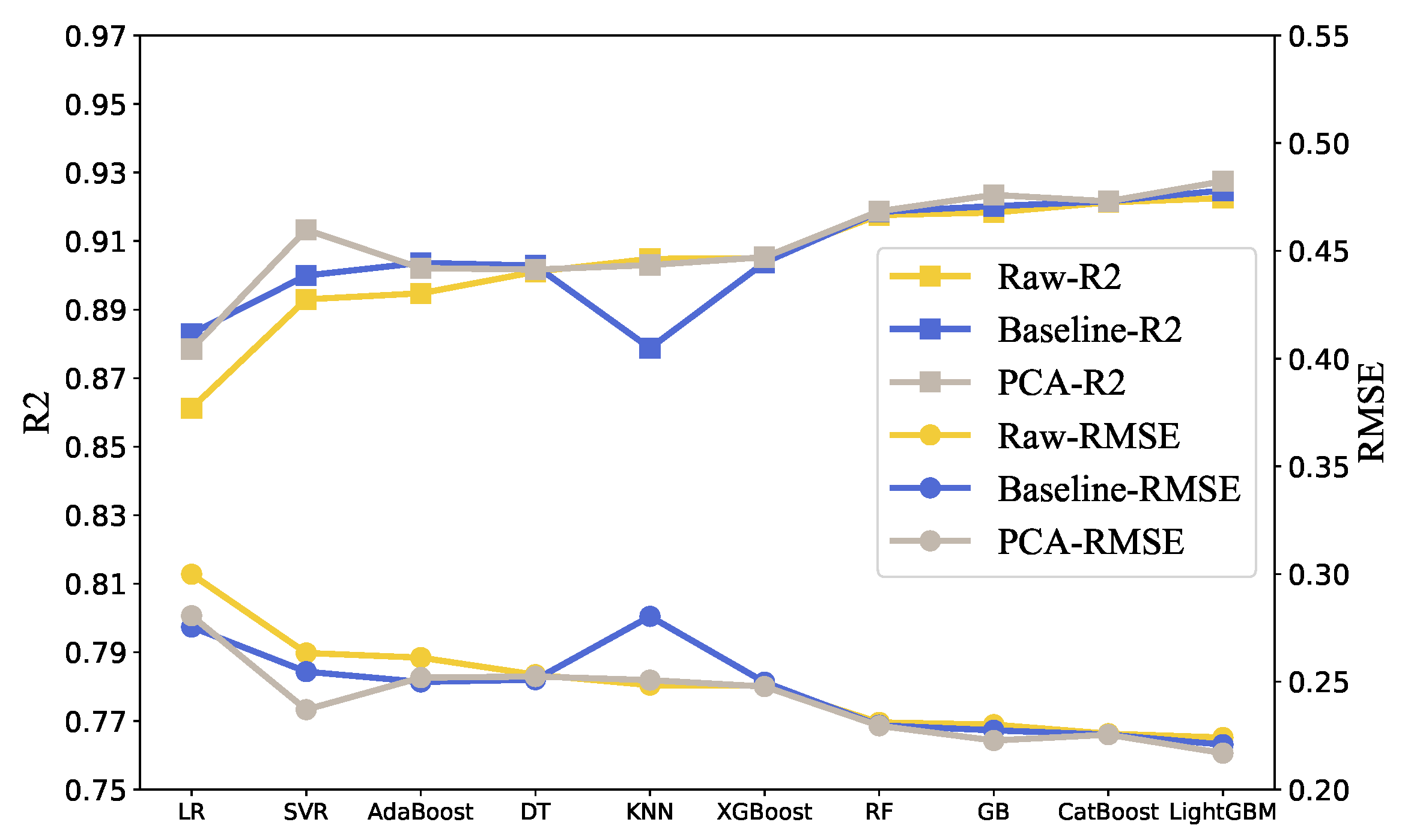
In order to remove redundant information from the input characteristics, the dimensionality of the material properties was reduced in this study. Principal component analysis is a multivariate statistical method used to investigate the correlation between multiple variables [19]. PCA dimensionality reduction was applied to material features. When 90% of the information was retained, the principal components were obtained. Then, the training set was re-organized and imported into the training model. In this way, the and of each model on the verification set were obtained, and the RMSE comparison results are shown in Figure 4.
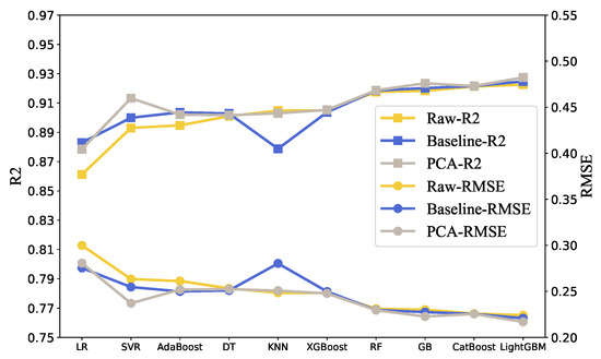
Figure 4.
Dimensionality reduction experiment results.
In most models with the same control parameters, the of the data set was higher and was lower. As a consequence, PCA dimensionality reduction decreased the redundant information in the data to a certain extent, and improved the fitting of the model to the data. Therefore, based on the results, the feature fusion of material properties can improve the stability and reliability of the model. In addition, during model training, the hyperparameters of the three groups of comparative experimental models were identical. In the following experiments, different feature selection experiments on different models were further carried out to fuse data features.
3.2. Feature Selection Experiment
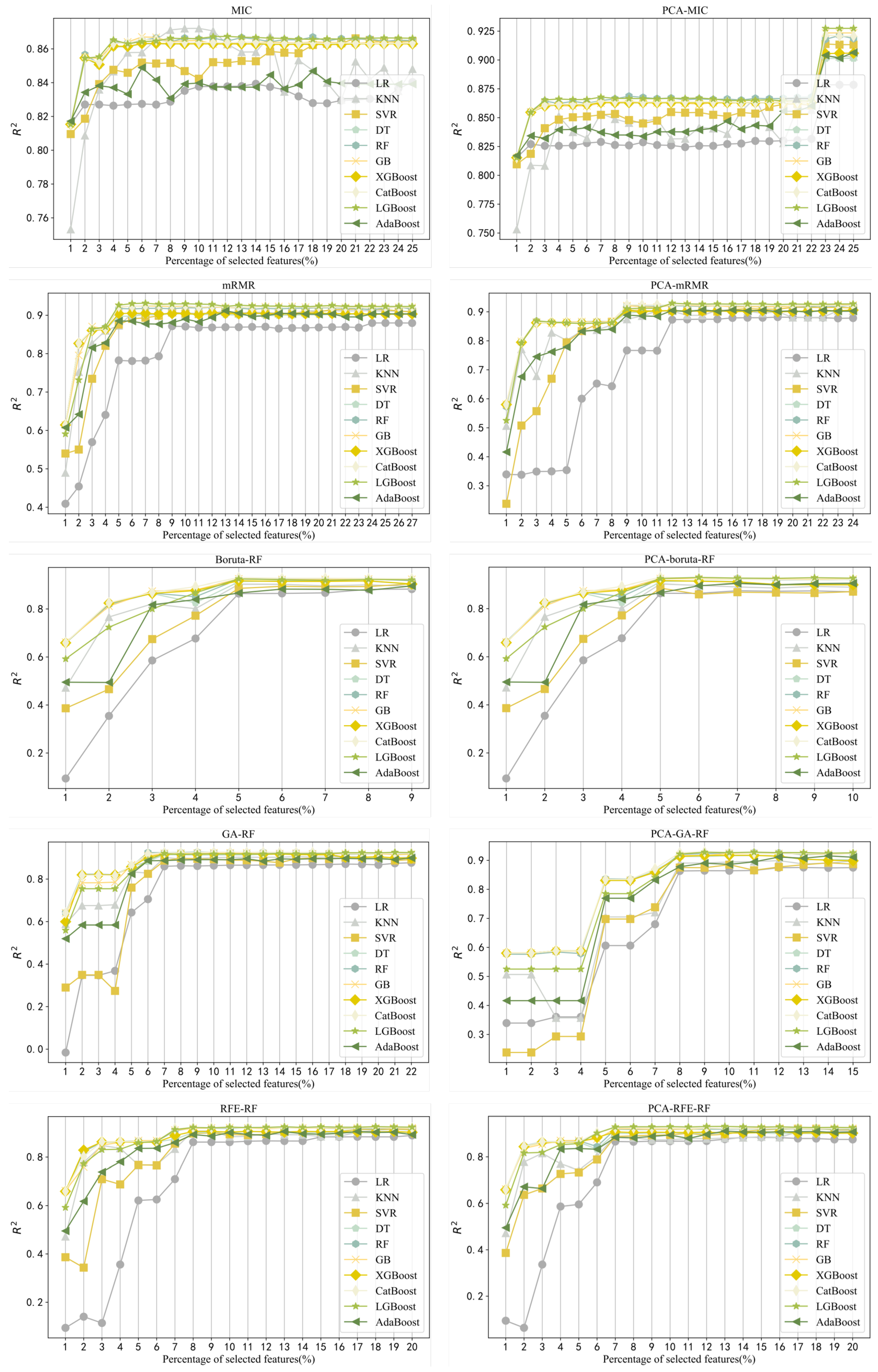
Redundant or irrelevant information in the sample affects the prediction performance of the regression model. Feature selection is the process of selecting the most effective subsets of prediction targets to reduce the dimension of the feature space [20]. Based on the greedy strategy, feature selection experiments were conducted on two sets of data sets. The feature selection methods included MIC, MRMR, Boruta, RFE, and the intelligent optimization method GA. Feature selection experiments were carried out on 10 machine learning models, with the optimization goal of maximizing .
The specific experimental results are shown in Table 2, where the represents the number of selected representative process parameter features and represents the number of material features selected. The visualization of the experimental results is shown in Figure 5. In Table 2, the optimal feature subset under different feature selection methods for the same model corresponds to the number of process parameters and the number of material features. These process parameters are closely related to the nugget quality [21], which is in line with actual production experience. Meanwhile, material features in several different feature subsets also account for a large proportion, demonstrating that material features are extremely important.

Table 2.
The optimal feature subset under different feature selection methods for the same model corresponds to the number of process parameters and the number of material features. Bold represents the best result.
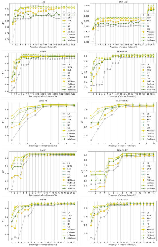
Figure 5.
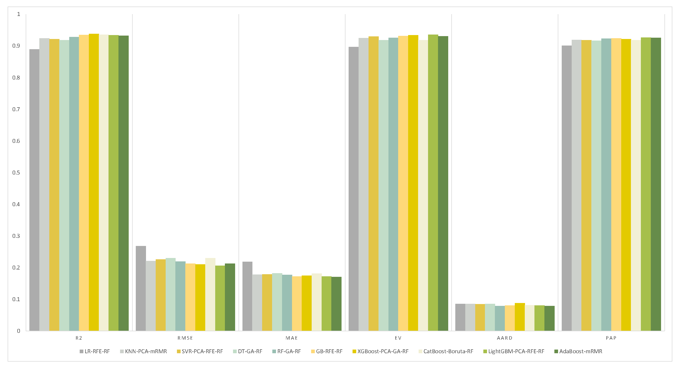
Index results.
As can be seen from Figure 5, the larger the dimension of the feature subset, the stronger the fitting ability of the model to the data. Moreover, based on the characteristics of data processed by different models, the model fitting ability is not always stronger after the dimensionality reduction of material features. Therefore, it is greatly necessary to select and compare the features of the two groups of data.
According to the fitting ability on the two sets of data sets, each machine learning model obtained the corresponding optimal subset through feature selection. In the next section, the hyperparameter optimization of each model on the two sets of data sets is detailed.
3.3. Hyperparameter Optimization and Quality Prediction
In this study, the hyperparameters of the models were optimized using the Bayesian algorithm for the optimal subsets of different models and through maximizing the on the verification set as the objective function, allowing us to finally obtain a series of optimal feature selection methods for different models. According to our experimental results, different models were equipped with different optimal feature selection methods. For example, the best feature selection method for Multi-LR was RFE, while the best feature selection method for KNN was MRMR. The correspondences are shown in Figure 6.

Figure 6.
Feature selection comparison: (a) process parameter; (b) feature fusion.
The evaluation indices of each model on the best feature subsets were calculated. The results are presented in Table 3 and the visualization is shown in Figure 7. In comparison, on the feature fusion data set, the XGBoost model selected with GA features realized the most outstanding performance in the three indices of , , and . The LightGBM model selected with RFE features exhibited the highest PAP value. In the non-dimensionality reduction model, the MAE value of the CatBoost model selected with Boruta features was the smallest, while the value of the random forest model selected with GA features was the smallest.

Table 3.
The evaluation indices of each model on the best feature subsets. Bold represents the best result.
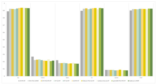
Figure 7.
Testing results.
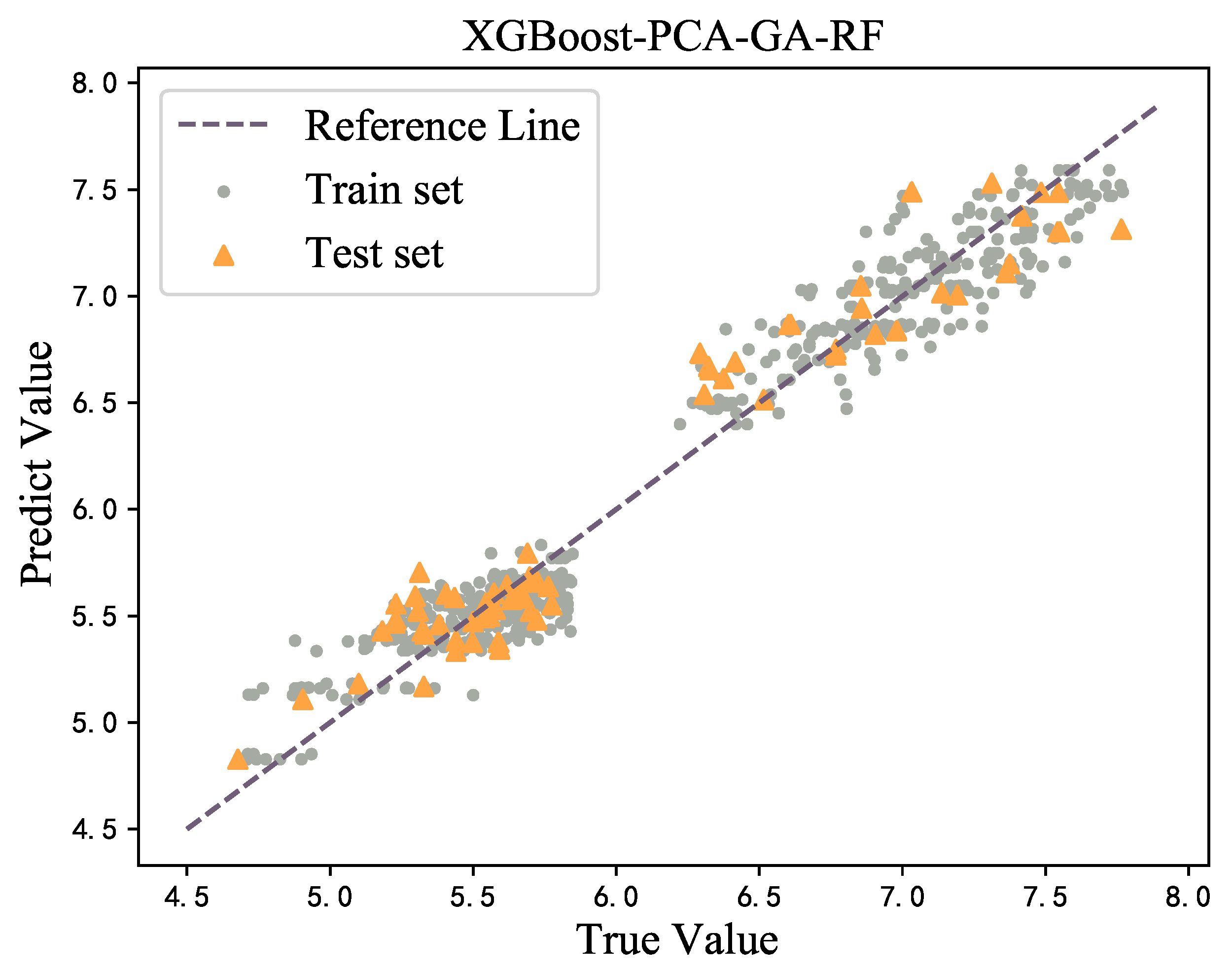
For the trained model, regression prediction was performed on both the training set and the verification set, and the visualization of the results is provided in Figure 8. It can be seen that the fitting effect of the XGBoost model was good and there was no obvious large number of outliers in each model, indicating that no overfitting phenomenon is observed.
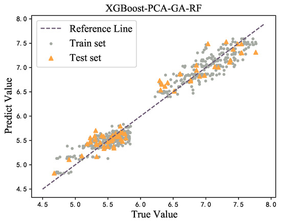
Figure 8.
Prediction on training set and testing set.
4. Conclusions
In this study, three kinds of data sets—including original data, fusion material characteristic data, and material characteristic PCA feature dimensionality reduction fusion data—were used to train 10 machine learning algorithms for the prediction of the nugget diameter of RSW. In addition, the effects of the Bayesian optimization method and five feature selection methods on the model were studied and compared, considering the maximum mutual information coefficient, maximum correlation and minimum redundancy coefficient, Boruta, recursive feature elimination, and genetic algorithm. Furthermore, the , , , , , and were used as comprehensive evaluation indices for the models. The experimental results revealed the following:
- The prediction model trained using a genetic algorithm combined with the Bayesian Optimization XGBoost algorithm can predict the size of nugget very accurately, and the complexity and inconsistency of data will not affect its prediction performance. Moreover, the Bayesian optimization method is completely effective for hyperparameter optimization and the regulation of overfitting.
- Through adding the mechanical properties and chemical element contents of materials into the feature set, and reducing its dimensionality using PCA to conduct feature fusion, the performance of the model can be effectively improved. For example, compared with the original data, the of the XGBoost model was enhanced by 3.2%.
Through these experimental results, the following conclusions can be drawn:
- Material features impose a great impact on the prediction performance of the model. All feature selection methods added a certain proportion of material features to the feature subsets of the two data sets. In particular, electrode pressure, welding current, and welding time were included in all feature subsets. The three process parameters are of great importance for nugget formation, which is consistent with actual welding experience and theory.
- The PCA method can effectively remove redundant information of material characteristics. The four feature selection methods—consisting of maximum correlation minimum redundancy coefficient, Boruta, recursive feature elimination, and genetic algorithm—were applied to several machine learning models, and the performance of the machine learning algorithms was improved to varying degrees. Therefore, it is crucial to select and obtain the optimal feature subset using feature selection methods.
- The results revealed that the proportional increase or decrease in material features in different feature subsets is not stable. In fact, the heat generated during resistance spot-welding obeys Joule’s Law. Material characteristics are particularly critical for nugget formation, and the current has a greater impact on heat with an increase in time. While the disadvantage is that the dynamic resistance in the actual nugget formation process changes within a certain range, it is regarded as a fixed value for analysis in this paper. Therefore, there is a certain error with respect to the actual situation. In order to reduce this error, the maximum mutual information coefficient was adopted for feature selection, and the features were sorted and selected according to the size of the maximum mutual information coefficient. For the purpose of controlling the number of features selected with each feature selection method to be close to the same, it is sufficient to retain the first 20 dimensional features at most.
- This investigation was limited to the consideration of static process parameters and material properties, without real-time dynamic monitoring of the welding process. A promising avenue for future research is to exploit the wealth of data generated by internal sensors within the welding machine (e.g., current, voltage, and displacement sensors) and external environmental sensors (e.g., temperature and humidity sensors), and to integrate these data streams using advanced data fusion techniques to improve the accuracy of predictions.
Author Contributions
All authors contributed to the study conception and design. Q.Z. performed the experiment, data collection, analysis and contributed to manuscript preparation; H.S. contributed to manuscript preparation and wrote the manuscript; X.Z. contributed to the experiment and manuscript preparation; Y.W. helped perform the analysis with constructive discussions. All authors have read and agreed to the published version of the manuscript.
Funding
This work was supported in part by the National Key Research and Development Program of China under Grant 2020YFB1710700.
Data Availability Statement
Data are contained within the article.
Conflicts of Interest
Authors Qinmiao Zhu and Yuhui Wang were employed by the company Wuhan Digital Design and Manufacturing Innovation Center Co., Ltd. Author Xiaohui Zhu was employed by the company Wuhan Huaweike Intelligent Technology Co., Ltd. The remaining authors declare that the research was conducted in the absence of any commercial or financial relationships that could be construed as a potential conflict of interest.
References
- Martin, O.; Ahedo, V.; Santos, J.I.; Galán, J.M. Comparative Study of Classification Algorithms for Quality Assessment of Resistance Spot Welding Joints From Pre-and Post-Welding Inputs. IEEE Access 2022, 10, 6518–6527. [Google Scholar] [CrossRef]
- Zhao, D.; Ivanov, M.; Wang, Y.; Liang, D.; Du, W. Multi-objective optimization of the resistance spot welding process using a hybrid approach. J. Intell. Manuf. 2021, 32, 2219–2234. [Google Scholar] [CrossRef]
- Vignesh, K.; Elaya Perumal, A.; Velmurugan, P. Resistance spot welding of AISI-316L SS and 2205 DSS for predicting parametric influences on weld strength—Experimental and FEM approach. Arch. Civ. Mech. Eng. 2019, 19, 1029–1042. [Google Scholar] [CrossRef]
- Bae, J.H.; Park, Y.D.; Lee, M. Optimization of Welding Parameters for Resistance Spot Welding of AA3003 to Galvanized DP780 Steel Using Response Surface Methodology. Int. J. Automot. Technol. 2021, 22, 585–593. [Google Scholar] [CrossRef]
- Vigneshkumar, M.; Varthanan, P.A. Comparison of RSM and ANN model in the prediction of the tensile shear failure load of spot welded AISI 304/316 L dissimilar sheets. Int. J. Comput. Mater. Sci. Surf. Eng. 2019, 8, 114–130. [Google Scholar] [CrossRef]
- Hoseini, H.T.; Farahani, M.; Sohrabian, M. Process analysis of resistance spot welding on the Inconel alloy 625 using artificial neural networks. Int. J. Manuf. Res. 2017, 12, 444–460. [Google Scholar] [CrossRef]
- Chen, F.; Wang, Y.; Sun, S.; Ma, Z.; Huang, X. Multi-objective optimization of mechanical quality and stability during micro resistance spot welding. Int. J. Adv. Manuf. Technol. 2019, 101, 1903–1913. [Google Scholar] [CrossRef]
- Zamanzad Gavidel, S.; Lu, S.; Rickli, J.L. Performance analysis and comparison of machine learning algorithms for predicting nugget width of resistance spot welding joints. Int. J. Adv. Manuf. Technol. 2019, 105, 3779–3796. [Google Scholar] [CrossRef]
- Lee, S.; Kareem, A.B.; Hur, J.W. A Comparative Study of Deep-Learning Autoencoders (DLAEs) for Vibration Anomaly Detection in Manufacturing Equipment. Electronics 2024, 13, 1700. [Google Scholar] [CrossRef]
- Cheadle, C.; Vawter, M.P.; Freed, W.J.; Becker, K.G. Analysis of microarray data using Z score transformation. J. Mol. Diagn. 2003, 5, 73–81. [Google Scholar] [CrossRef] [PubMed]
- Zhou, K.; Cai, L. Online nugget diameter control system for resistance spot welding. Int. J. Adv. Manuf. Technol. 2013, 68, 2571–2588. [Google Scholar] [CrossRef]
- Gomez, J.C.; Moens, M.F. PCA document reconstruction for email classification. Comput. Stat. Data Anal. 2012, 56, 741–751. [Google Scholar] [CrossRef]
- Reshef, D.N.; Reshef, Y.A.; Finucane, H.K.; Grossman, S.R.; McVean, G.; Turnbaugh, P.J.; Lander, E.S.; Mitzenmacher, M.; Sabeti, P.C. Detecting novel associations in large data sets. Science 2011, 334, 1518–1524. [Google Scholar] [CrossRef] [PubMed]
- Peng, H.; Long, F.; Ding, C. Feature selection based on mutual information criteria of max-dependency, max-relevance, and min-redundancy. IEEE Trans. Pattern Anal. Mach. Intell. 2005, 27, 1226–1238. [Google Scholar] [CrossRef] [PubMed]
- Kursa, M.B.; Jankowski, A.; Rudnicki, W.R. Boruta—A system for feature selection. Fundam. Informaticae 2010, 101, 271–285. [Google Scholar] [CrossRef]
- Guyon, I.; Weston, J.; Barnhill, S.; Vapnik, V. Gene selection for cancer classification using support vector machines. Mach. Learn. 2002, 46, 389–422. [Google Scholar] [CrossRef]
- Hou, Y.; Yang, A.; Guo, W.; Zheng, E.; Xiao, Q.; Guo, Z.; Huang, Z. Bearing Fault Diagnosis Under Small Data Set Condition: A Bayesian Network Method With Transfer Learning for Parameter Estimation. IEEE Access 2022, 10, 35768–35783. [Google Scholar] [CrossRef]
- Wang, W.R.; Wang, W.L.; Wang, S.C.; Tsai, Y.C.; Lai, C.H.; Yeh, J.W. Effects of Al addition on the microstructure and mechanical property of AlxCoCrFeNi high-entropy alloys. Intermetallics 2012, 26, 44–51. [Google Scholar] [CrossRef]
- Abdi, H.; Williams, L.J. Principal component analysis. Wiley Interdiscip. Rev. Comput. Stat. 2010, 2, 433–459. [Google Scholar] [CrossRef]
- Kira, K.; Rendell, L.A. The feature selection problem: Traditional methods and a new algorithm. In Proceedings of the Aaai, San Jose, CA, USA, 12–16 July 1992; Volume 2, pp. 129–134. [Google Scholar]
- Arunchai, T.; Sonthipermpoon, K.; Apichayakul, P.; Tamee, K. Resistance spot welding optimization based on artificial neural network. Int. J. Manuf. Eng. 2014, 2014, 154784. [Google Scholar] [CrossRef]
Disclaimer/Publisher’s Note: The statements, opinions and data contained in all publications are solely those of the individual author(s) and contributor(s) and not of MDPI and/or the editor(s). MDPI and/or the editor(s) disclaim responsibility for any injury to people or property resulting from any ideas, methods, instructions or products referred to in the content. |
© 2024 by the authors. Licensee MDPI, Basel, Switzerland. This article is an open access article distributed under the terms and conditions of the Creative Commons Attribution (CC BY) license (https://creativecommons.org/licenses/by/4.0/).

