Manifold Optimization-Based Data Detection Algorithm for Multiple-Input–Multiple-Output Orthogonal Frequency-Division Multiplexing Systems under Time-Varying Channels

Abstract

Recently, multiple-input–multiple-output (MIMO) orthogonal frequency-division multiplexing (OFDM) systems have gained significant attention in the field of wireless communications. The utilization of the Riemannian manifold has become prevalent in MIMO-OFDM systems. However, the existing data detection algorithms for MIMO-OFDM systems are mostly designed for block fading channels. Additionally, these algorithms often suffer from high computational complexity. In this paper, we propose a data detection algorithm on the basis of Riemannian manifold optimization for MIMO-OFDM systems under time-varying channels. The core concept of this algorithm is to optimize the transmitted signals by solving the manifold optimization problem in the case of time-varying channels. In order to reduce the computational complexity of the algorithm, we improve the proposed algorithm by dividing the transmitted signals into multiple subframes for solving the optimization problem separately and using the pilots to maintain the performance of the algorithm. In the simulation, the performance of multiple proposed algorithms and the forced-zero detection algorithm under different parameter settings are compared. The simulation results show that the proposed algorithm demonstrates good bit error rate and computational complexity performances.

1. Introduction

Multiple-input–multiple-output (MIMO) orthogonal frequency-division multiplexing (OFDM) technology plays an important role in fifth-generation mobile communication systems, enabling enhanced spectrum efficiency and transmission rates in wireless communications [1,2]. Compared with single-input–single-output systems, MIMO systems require multiple signals to be transmitted, resulting in a significant increase in the number of channels. Consequently, data detection becomes more challenging and crucial for MIMO-OFDM systems.

Extensive research has been conducted on data detection techniques for MIMO-OFDM systems, with a focus on achieving higher performance while reducing complexity. In [3], linear estimation methods are analyzed, including data detection on the basis of the ZF criterion and the MMSE criterion. In Ref. [4], subspace is used for data detection for MIMO-OFDM systems. This subspace identification algorithm can achieve good estimation performance in scenarios where the channel does not change rapidly. However, it fails to work effectively in situations with rapid channel variations. Ref. [5] employs Monte Carlo methods and iterative approaches to jointly estimate the channel and signals for MIMO-OFDM systems. Ref. [6] analyzes MIMO-OFCDM with zero-forcing successive interference cancellation and imperfect channel estimation. This approach takes into account the correlation between errors, making it more accurate than methods that do not consider such correlation. Ref. [7] propose a joint iterative detection for the MIMO-OFCDM system, which enables space and frequency diversity gains to be jointly exploited. As the number of detections increases and the frequency domain expansion factor grows, the performance improvement becomes more significant. Ref. [8] propose an iterative algorithm based on the variational Bayesian inference framework to address the signal detection problem in OFDM-V-MIMO systems under severe communication environments.

In recent years, manifold optimization has gained significant attention and has found wide application in various fields, including data detection [9]. The main idea of Riemannian manifold optimization is if the constraints in an optimization problem possess certain geometric properties, these constraints can be used to construct a Riemannian manifold. Then, gradient descent search can be performed directly on this Riemannian manifold, without the need for computations in the standard Euclidean space. Applying the method of Riemannian manifold optimization can transform a constrained optimization problem into an unconstrained optimization problem on the manifold. Subsequently, unconstrained optimization algorithms based on gradient descent can be used to solve the optimization problem on the Riemannian manifold. This optimization method is equivalent to solving the optimization problem directly in the Euclidean space. Ref. [10] applies manifold learning to channel state information reconstruction. Manifold learning can recover low-dimensional manifolds from high-dimensional spaces while preserving the inherent manifold structure of the data. In [11], a manifold optimization-based data detection method for massive multiuser MIMO has been proposed. This method utilizes manifolds and converts the constrained optimization problem into an unconstrained problem on this manifold. It directly employs the gradient descent method for searching. Ref. [12] introduces a manifold-based joint channel estimation and signal detection method for MIMO, which converts the data detection problem into a manifold optimization problem in the real domain. Although the above methods maintain low algorithm complexity, they are only applicable to MIMO systems with block fading channels. In [13], Riemannian manifold optimization is applied to hybrid beamforming to ensure the beamforming required for radar sensing. It has achieved good results in the radar fields, with high computational efficiency and nearly optimal performance. Ref. [14] applies Riemannian manifold optimization to reflective surface coefficient optimization. The Riemannian manifold algorithm can converge within a relatively small number of iterations, resulting in low computational complexity and significantly reduced computation time.

In this paper, we propose a manifold optimization data detection algorithm which is able to be applied to MIMO-OFDM systems with rapidly changing channels. Specifically, we derive the manifold optimization problem for time-varying channel scenarios. We use a GAN-based method to obtain the initial estimate of the channels, and then use the zero-forcing (ZF) detection to obtain the initial estimation of the transmitted signals. To reduce the complexity of solving the proposed optimization problem, we divide a data frame into several subframes, each contains several OFDM symbols, and then solve the optimization problem in subframe units. Pilot symbols are utilized to evaluate the estimated signals and determine the termination condition for the optimization process. The simulation results show that the proposed algorithm achieves better BER performance than the algorithm that uses an estimated channel for ZF detection while maintaining low computational complexity.

The rest of the paper is organized as follows. Section 2 presents the system model of MIMO-OFDM systems. Section 3 describes the manifold optimization algorithm under time-invariant channels. Section 4 describes the proposed manifold optimization-based data detection algorithm for MIMO-OFDM systems under time-varying channels, including problem formulation and complexity reduction. The results of the simulations are presented in Section 5, and the conclusions are presented in Section 6.

2. System Model

This paper considers a MIMO-OFDM system with $N_t$ transmit antennas and $N_r$ receive antennas, operating on K subcarriers. Each data frame of the transmitted signal contains $N_f$ OFDM symbols. Let $x_{n,k}^p$ represent the transmitted signal at the pth transmit antenna and the kth subcarrier of the nth OFDM symbol in one frame, where $1\le p\le N_t$, $1\le n\le N_t$, $1\le k\le K$, the average power $E\left\{{\left|x_{n,k}^p\right|}^2\right\}={\sigma }_x^2$, and $E\left\{·\right\}$ denotes the expectation. The transmitted signal propagates through the channel and arrives at the receiving side, where the received signals are the sum of transmitted signals and noise. The transmitted signal at the qth receive antenna and the kth subcarrier of the nth OFDM symbol can be expressed as

$$y_{n,k}^q=\sum _{p=1}^{N_t}{h}_{n,k}^{q,p}{x}_{n,k}^p+w_{n,k}^q,$$

(1)

where $1\le q\le N_r$, $h_{n,k}^{q,p}$ represents the channel frequency response between the pth transmit antenna and the qth receive antenna at the kth subcarrier of the nth OFDM symbol, $x_{n,k}^p$ and $y_{n,k}^q$ are the frequency domain representations of the transmitted and received signals, respectively, and $w_{n,k}^q$ is a complex Gaussian noise sample with zero mean and variance ${\sigma }_w^2$.

By defining ${\mathit{x}}_{n,k}={\left[\begin{array}{cccc}{x}_{n,k}^1& x_{n,k}^2& \cdots & x_{n,k}^{N_t}\end{array}\right]}^T\in {\mathbb{C}}^{N_t\times 1}$, ${\mathit{y}}_{n,k}={\left[\begin{array}{cccc}{y}_{n,k}^1& y_{n,k}^2& \cdots & y_{n,k}^{N_r}\end{array}\right]}^T\in {\mathbb{C}}^{N_r\times 1}$, ${\mathit{w}}_{n,k}={\left[\begin{array}{cccc}{w}_{n,k}^1& w_{n,k}^2& \cdots & w_{n,k}^{N_r}\end{array}\right]}^T\in {\mathbb{C}}^{N_r\times 1}$, ${\mathit{H}}_{n,k}={\left[\begin{array}{cccc}{\mathit{h}}_{n,k}^1& {\mathit{h}}_{n,k}^2& \cdots & {\mathit{h}}_{n,k}^{N_r}\end{array}\right]}^T\in {\mathbb{C}}^{N_r\times N_t}$, and ${\mathit{h}}_{n,k}^q={\left[\begin{array}{cccc}{h}_{n,k}^{q,1}& h_{n,k}^{q,2}& \cdots & h_{n,k}^{q,N_t}\end{array}\right]}^T\in {\mathbb{C}}^{N_t\times 1}$, where ${(·)}^T$ stands for transpose, (1) can be represented as follows:

$$\begin{array}{c}\hfill {\mathit{y}}_{n,k}={\mathit{H}}_{n,k}{\mathit{x}}_{n,k}+{\mathit{w}}_{n,k}.\end{array}$$

(2)

3. Conventional Data Detection Algorithm Based on Manifold Optimization

In this section, the conventional data detection algorithm for MIMO-OFDM systems based on manifold optimization is presented. Here, it is assumed that the channel is constant in a frame, i.e., ${\mathit{H}}_{1,k}=\cdots ={\mathit{H}}_{N_f,k}={\mathit{H}}_k$.

By collecting all the data at the kth subcarriers in one frame, we can obtain

$$\begin{array}{c}\hfill {\mathit{Y}}_k={\mathit{H}}_k{\mathit{X}}_k+{\mathit{W}}_k,\end{array}$$

(3)

where ${\mathit{X}}_k=\left[\begin{array}{cccc}{\mathit{x}}_{1,k}& {\mathit{x}}_{2,k}& \cdots & {\mathit{x}}_{N_f,k}\end{array}\right]\in {\mathbb{C}}^{N_t\times N_f}$, ${\mathit{Y}}_k=\left[\begin{array}{cccc}{\mathit{y}}_{1,k}& {\mathit{y}}_{2,k}& \cdots & {\mathit{y}}_{N_f,k}\end{array}\right]\in {\mathbb{C}}^{N_r\times N_f}$, and ${\mathit{W}}_k=\left[\begin{array}{cccc}{\mathit{w}}_{1,k}& {\mathit{w}}_{2,k}& \cdots & {\mathit{w}}_{N_f,k}\end{array}\right]\in {\mathbb{C}}^{N_r\times N_f}$.

Given ${\mathit{Y}}_k$, the joint estimation of ${\mathit{X}}_k$ and ${\mathit{H}}_k$ can be formulated as the following optimization problem [12]:

$$\begin{array}{c}\hfill \underset{{\mathit{H}}_k,{\mathit{X}}_k}{\min }J({\mathit{H}}_k,{\mathit{X}}_k)={∥{\mathit{Y}}_k-{\mathit{H}}_k{\mathit{X}}_k∥}_F^2,\end{array}$$

(4)

where ${∥·∥}_F$ denotes the Frobenius norm. Since the manifold is defined on the real number domain, the above optimization problem needs to be transformed into a real-valued representation, which is given by [12]

$$\begin{array}{c}\hfill \underset{{\overline{\mathit{H}}}_k,{\overline{\mathit{X}}}_k}{\min }J({\overline{\mathit{H}}}_k,{\overline{\mathit{X}}}_k)={∥{\overline{\mathit{Y}}}_k-{\overline{\mathit{H}}}_k{\overline{\mathit{X}}}_k∥}_F^2,\end{array}$$

(5)

where

$$\begin{array}{c}\hfill {\overline{\mathit{H}}}_k=\left[\begin{array}{cc}\mathrm{Re}\left({\mathit{H}}_k\right)& -\mathrm{Im}\left({\mathit{H}}_k\right)\\ \mathrm{Im}\left({\mathit{H}}_k\right)& \mathrm{Re}\left({\mathit{H}}_k\right)\end{array}\right]\in {\mathbb{R}}^{2N_r\times 2N_t},\end{array}$$

(6)

$$\begin{array}{c}\hfill {\overline{\mathit{Y}}}_k=\left[\begin{array}{c}\mathrm{Re}\left({\mathit{Y}}_k\right)\\ \mathrm{Im}\left({\mathit{Y}}_k\right)\end{array}\right]\in {\mathbb{R}}^{2N_r\times N_f},\end{array}$$

(7)

$$\begin{array}{c}\hfill {\overline{\mathit{X}}}_k=\left[\begin{array}{c}\mathrm{Re}\left({\mathit{X}}_k\right)\\ \mathrm{Im}\left({\mathit{X}}_k\right)\end{array}\right]\in {\mathbb{R}}^{2N_t\times N_f},\end{array}$$

(8)

$\mathrm{Re}(·)$ denotes the real part and $\mathrm{Im}(·)$ denotes the imaginary part.

We can obtain the optimal ${\overline{\mathit{X}}}_k$ and ${\overline{\mathit{H}}}_k$ by iterative solution of the optimization problem (5). Given ${\overline{\mathit{X}}}_k$, since ${\overline{\mathit{Y}}}_k={\overline{\mathit{H}}}_k{\overline{\mathit{X}}}_k+{\overline{\mathit{W}}}_k,$ where ${\overline{\mathit{W}}}_k=\left[\begin{array}{c}\mathrm{Re}\left({\mathit{W}}_k\right)\\ \mathrm{Im}\left({\mathit{W}}_k\right)\end{array}\right]\in {\mathbb{R}}^{2N_r\times N_f}$, the least squares estimation of ${\overline{\mathit{H}}}_k$ can be computed as

$$\begin{array}{c}\hfill {\widehat{\overline{\mathit{H}}}}_k={\overline{\mathit{Y}}}_k{\overline{\mathit{X}}}_k^T{\left({\overline{\mathit{X}}}_k{\overline{\mathit{X}}}_k^T\right)}^{-1}.\end{array}$$

(9)

Substituting (9) into (5), we can obtain the following simplified objective function:

$$\begin{array}{ll}J\left({\overline{\mathit{X}}}_k\right)& ={∥{\overline{\mathit{Y}}}_k-{\overline{\mathit{Y}}}_k{\overline{\mathit{X}}}_k^T{\left({\overline{\mathit{X}}}_k{\overline{\mathit{X}}}_k^T\right)}^{-1}{\overline{\mathit{X}}}_k∥}_F^2\\ \hfill & =\mathrm{trace}\left\{\left[{\overline{\mathit{Y}}}_k-{\overline{\mathit{Y}}}_k{\overline{\mathit{X}}}_k^T{\left({\overline{\mathit{X}}}_k{\overline{\mathit{X}}}_k^T\right)}^{-1}{\overline{\mathit{X}}}_k\right]{\left[{\overline{\mathit{Y}}}_k-{\overline{\mathit{Y}}}_k{\overline{\mathit{X}}}_k^T{\left({\overline{\mathit{X}}}_k{\overline{\mathit{X}}}_k^T\right)}^{-1}{\overline{\mathit{X}}}_k\right]}^T\right\}\\ \hfill & =\mathrm{trace}\left\{{\overline{\mathit{Y}}}_k{\overline{\mathit{Y}}}_k^T\right\}-\mathrm{trace}\left\{{\overline{\mathit{Y}}}_k{\overline{\mathit{X}}}_k^T{\left({\overline{\mathit{X}}}_k{\overline{\mathit{X}}}_k^T\right)}^{-1}{\overline{\mathit{X}}}_k{\overline{\mathit{Y}}}_k^T\right\},\hfill \end{array}$$

(10)

where $\mathrm{trace}\left\{·\right\}$ denotes the trace. Since $\mathrm{trace}\left\{{\overline{\mathit{Y}}}_k{\overline{\mathit{Y}}}_k^T\right\}$ is independent of the transmitted signal ${\overline{\mathit{X}}}_k$, the objective function can be further transformed into

$$F\left({\overline{\mathit{X}}}_k\right)=-\mathrm{trace}\left\{{\overline{\mathit{Y}}}_k{\overline{\mathit{X}}}_k^T{\left({\overline{\mathit{X}}}_k{\overline{\mathit{X}}}_k^T\right)}^{-1}{\overline{\mathit{X}}}_k{\overline{\mathit{Y}}}_k^T\right\}.$$

(11)

Since the transmitted signal ${\overline{\mathit{X}}}_k$ can be approximated to lie on a sphere manifold when the data length is sufficiently long [15], the optimization problem is eventually written in the following form:

$$\begin{array}{c}\underset{{\overline{\mathit{X}}}_k}{\min }F\left({\overline{\mathit{X}}}_k\right)=-\mathrm{trace}\left\{{\overline{\mathit{Y}}}_k{\overline{\mathit{X}}}_k^T{\left({\overline{\mathit{X}}}_k{\overline{\mathit{X}}}_k^T\right)}^{-1}{\overline{\mathit{X}}}_k{\overline{\mathit{Y}}}_k^T\right\},\hfill \\ \mathrm{s}.\mathrm{t}.{∥{\overline{\mathit{X}}}_k∥}_F=\sqrt{N_t{N}_f{\sigma }_x^2}.\hfill \end{array}$$

(12)

Equation (12) can be further expressed as the Riemannian optimization problem:

$$\begin{array}{c}\underset{{\overline{\mathit{S}}}_k}{\min }F\left({\overline{\mathit{S}}}_k\right)=-\mathrm{trace}\left\{{\overline{\mathit{Y}}}_k{\overline{\mathit{S}}}_k^T{\left({\overline{\mathit{S}}}_k{\overline{\mathit{S}}}_k^T\right)}^{-1}{\overline{\mathit{S}}}_k{\overline{\mathit{Y}}}_k^T\right\},\hfill \\ \mathrm{s}.\mathrm{t}.{∥{\overline{\mathit{S}}}_k∥}_F=1.\hfill \end{array}$$

(13)

where ${\overline{\mathit{X}}}_k=\sqrt{N_t{N}_f{\sigma }_x^2}{\overline{\mathit{S}}}_k$. After that, one can use the Riemannian conjugate gradient algorithm [16] to solve (13). Note that this algorithm needs the Euclidean gradient of $F\left({\overline{\mathit{S}}}_k\right)$, computed as

$$\begin{array}{cc}\hfill \mathrm{Grad}F\left({\overline{\mathit{S}}}_k\right)=& -2{\left({\overline{\mathit{S}}}_k{\overline{\mathit{S}}}_k^T\right)}^{-1}{\overline{\mathit{S}}}_k{\overline{\mathit{Y}}}_k^T{\overline{\mathit{Y}}}_k{\overline{\mathit{S}}}_k^T{\left({\overline{\mathit{S}}}_k{\overline{\mathit{S}}}_k^T\right)}^{-1}{\overline{\mathit{S}}}_k\hfill \\ & -2{\left({\overline{\mathit{S}}}_k{\overline{\mathit{S}}}_k^T\right)}^{-1}{\overline{\mathit{S}}}_k{\overline{\mathit{Y}}}_k^T{\overline{\mathit{Y}}}_k.\hfill \end{array}$$

(14)

And the Riemannian gradient can be obtained by utilizing the Euclidean gradient as follows:

$$\mathrm{grad}F\left({\overline{\mathit{S}}}_k\right)=\mathrm{Grad}F\left({\overline{\mathit{S}}}_k\right)-\mathrm{trace}\left({\overline{\mathit{S}}}_k^T·\mathrm{Grad}F\left({\overline{\mathit{S}}}_k\right)\right){\overline{\mathit{S}}}_k$$

(15)

After the solution ${\widehat{\overline{\mathit{S}}}}_k$ of (13) is obtained, the estimation of the transmitted signal can be given by

$$\begin{array}{c}\hfill {\widehat{\mathit{X}}}_{k,\mathrm{solution}}=\sqrt{N_t{N}_f{\sigma }_x^2}\left\{{\left[{\widehat{\overline{\mathit{S}}}}_k\right]}_{\left[1:N_t\right];:}+\mathrm{j}·{\left[{\widehat{\overline{\mathit{S}}}}_k\right]}_{\left[N_t+1:2N_t\right];:}\right\},\end{array}$$

(16)

where ${\left[\mathit{A}\right]}_{\left[m:n\right];:}$ denotes taking the mth to nth rows of the matrix $\mathit{A}$.

With ${\widehat{\mathit{X}}}_{k,\mathrm{solution}}$, the final channel estimation ${\widehat{\mathit{H}}}_k$ can be obtained as

$${\widehat{\mathit{H}}}_k={\mathit{Y}}_k{\widehat{\mathit{X}}}_{k,\mathrm{solution}}^H{\left({\widehat{\mathit{X}}}_{k,\mathrm{solution}}{\widehat{\mathit{X}}}_{k,\mathrm{solution}}^H\right)}^{-1}.$$

(17)

In order to make the performance of data detection more enhanced, the final channel estimation can be used to estimate the signal again. That is, given ${\widehat{\mathit{H}}}_k$, one can obtain the final estimation of the transmitted signal as

$${\widehat{\mathit{X}}}_k=\mathrm{hard}\left\{{\left({\widehat{\mathit{H}}}_k^H{\widehat{\mathit{H}}}_k\right)}^{-1}{\widehat{\mathit{H}}}_k^H{\mathit{Y}}_k\right\}.$$

(18)

Choosing a good initial value is helpful for solving the optimization problem. To obtain a good initial value of (13), i.e., ${\widehat{\overline{\mathit{S}}}}_{k,\mathrm{ini}}$, $N_t$ OFDM symbols are used as pilot sequences to obtain the initial LS estimation of the channel, i.e.,

$$\begin{array}{c}\hfill {\widehat{\mathit{H}}}_{k,\mathrm{ini}}={\mathit{Y}}_{k,\mathrm{pilot}}{\mathit{X}}_{k,\mathrm{pilot}}^H{\left({\mathit{X}}_{k,\mathrm{pilot}}{\mathit{X}}_{k,\mathrm{pilot}}^H\right)}^{-1},\end{array}$$

(19)

where ${\mathit{X}}_{k,\mathrm{pilot}}=\left[\begin{array}{cccc}{\mathit{x}}_{1,k}& {\mathit{x}}_{2,k}& \cdots & {\mathit{x}}_{N_t,k}\end{array}\right]\in {\mathbb{C}}^{N_t\times N_t}$, ${\mathit{Y}}_{k,\mathrm{pilot}}={\mathit{H}}_k{\mathit{X}}_{k,\mathrm{pilot}}+{\mathit{W}}_{k,\mathrm{pilot}}=\left[\begin{array}{cccc}{\mathit{y}}_{1,k}& {\mathit{y}}_{2,k}& \cdots & {\mathit{y}}_{N_t,k}\end{array}\right]\in {\mathbb{C}}^{N_r\times N_t}$, and ${(·)}^H$ denotes conjugate transpose. Based on ${\widehat{\mathit{H}}}_{k,\mathrm{ini}}$, the initial estimation of ${\mathit{X}}_k$ can be obtained by using the ZF detection as

$${\widehat{\mathit{X}}}_{k,\mathrm{ini}}=\mathrm{hard}\left\{{\left({\widehat{\mathit{H}}}_{k,\mathrm{ini}}^H{\widehat{\mathit{H}}}_{k,\mathrm{ini}}\right)}^{-1}{\widehat{\mathit{H}}}_{k,\mathrm{ini}}^H{\mathit{Y}}_k\right\},$$

(20)

where $\mathrm{hard}\left\{·\right\}$ stands for hard-decisioning. Based on ${\widehat{\mathit{X}}}_{k,\mathrm{ini}}$, ${\widehat{\overline{\mathit{X}}}}_{k,\mathrm{ini}}$ can be obtained according to (8), where ${\overline{\mathit{X}}}_k$ and ${\mathit{X}}_k$ are replaced by ${\widehat{\overline{\mathit{X}}}}_{k,\mathrm{ini}}$ and ${\widehat{\mathit{X}}}_{k,\mathrm{ini}}$, respectively. Then, ${\widehat{\overline{\mathit{S}}}}_{k,\mathrm{ini}}$ can be obtained as

$${\widehat{\overline{\mathit{S}}}}_{k,\mathrm{ini}}=\frac{1}{\sqrt{N_t{N}_f{\sigma }_x^2}}{\widehat{\overline{\mathit{X}}}}_{k,\mathrm{ini}}.$$

(21)

The entire signal detection process is summarized as Algorithm 1.

Algorithm 1 Data detection algorithm based on manifold optimization for time-invariant channels.

1: Input: ${\left\{{\mathit{X}}_{k,\mathrm{pilot}}\right\}}_{k=1}^K$, ${\left\{{\mathit{Y}}_{k,\mathrm{pilot}}\right\}}_{k=1}^K$, ${\left\{{\mathit{Y}}_k\right\}}_{k=1}^K$ 2: Output: ${\left\{{\widehat{\mathit{X}}}_k\right\}}_{k=1}^K$ 3: for $k=1$ to K do 4:     (1) Obtain the initial channel estimation ${\widehat{\mathit{H}}}_{k,\mathrm{ini}}$ as (19); 5:     (2) Obtain the initial value ${\widehat{\overline{\mathit{S}}}}_{k,\mathrm{ini}}$ as (21); 6:     (3) Solve (13) by using the Riemannian conjugate gradient algorithm to obtain ${\widehat{\overline{\mathit{S}}}}_k$; 7:     (4) Obtain ${\widehat{\mathit{X}}}_{k,\mathrm{solution}}$ as (16); 8:     (5) Obtain the final signal estimation ${\widehat{\mathit{X}}}_k$ according to (17) and (18). 9: end for

4. Proposed Manifold Optimization-Based Data Detection Algorithm for MIMO-OFDM Systems Under Time-Varying Channels

The algorithm in Section 3 is only applicable to the scenarios where the channels are constant within one frame. However, in practice, channels are time-varying from one OFDM block to another. Therefore, considering time-varying channels, we propose a manifold optimization-based data detection algorithm for MIMO-OFDM systems in this section.

4.1. Problem Formulation and Solving

By collecting the received signals at all subcarriers of the nth symbol, we obtain

$${\mathit{Y}}_n={\mathit{H}}_n{\mathit{X}}_n+{\mathit{W}}_n,$$

(22)

where ${\mathit{Y}}_n=\mathrm{diag}\left\{\left[\begin{array}{cccc}{\mathit{y}}_{n,1}& {\mathit{y}}_{n,2}& \cdots & {\mathit{y}}_{n,K}\end{array}\right]\right\}\in {\mathbb{C}}^{K{N}_r\times K}$, ${\mathit{X}}_n=\mathrm{diag}\left\{\left[\begin{array}{cccc}{\mathit{x}}_{n,1}& {\mathit{x}}_{n,2}& \cdots & {\mathit{x}}_{n,K}\end{array}\right]\right\}\in {\mathbb{C}}^{K{N}_t\times K}$, ${\mathit{W}}_n=\mathrm{diag}\left\{\left[\begin{array}{cccc}{\mathit{w}}_{n,1}& {\mathit{w}}_{n,2}& \cdots & {\mathit{w}}_{n,K}\end{array}\right]\right\}\in {\mathbb{C}}^{K{N}_r\times K}$,

$${\mathit{H}}_n=\mathrm{diag}\left\{\left[\begin{array}{cccc}{\mathit{H}}_{n,1}& {\mathit{H}}_{n,2}& \cdots & {\mathit{H}}_{n,K}\end{array}\right]\right\}\in {\mathbb{C}}^{K{N}_r\times K{N}_t},$$

(23)

$$\mathrm{diag}\left\{\left[\begin{array}{cccc}{\mathit{A}}_1& {\mathit{A}}_2& \cdots & {\mathit{A}}_K\end{array}\right]\right\}\triangleq \left[\begin{array}{cccc}{\mathit{A}}_1& \mathit{0}& \cdots & \mathit{0}\\ \mathit{0}& {\mathit{A}}_2& \cdots & \mathit{0}\\ ⋮& ⋮& \ddots & ⋮\\ \mathit{0}& \mathit{0}& \cdots & {\mathit{A}}_K\end{array}\right],$$

(24)

and ${\mathit{A}}_k$ denotes a matrix or vector. Considering all $N_f$ OFDM symbols in one frame, we formulate the objective function as

$$\begin{array}{c}\hfill J({\mathit{X}}_1,\cdots ,{\mathit{X}}_{N_f})=\sum _{n=1}^{N_f}{∥{\mathit{Y}}_n-{\mathit{H}}_n{\mathit{X}}_n∥}_F^2.\end{array}$$

(25)

Similarly to Section 3, we transform the optimization problem into a real-valued representation, which is given by

$$J({\dot{\mathit{X}}}_1,\cdots ,{\dot{\mathit{X}}}_{N_f})=\sum _{n=1}^{N_f}{∥{\dot{\mathit{Y}}}_n-{\dot{\mathit{H}}}_n{\dot{\mathit{X}}}_n∥}_F^2.$$

(26)

where

$$\begin{array}{c}\hfill {\dot{\mathit{X}}}_n=\mathrm{diag}\left\{\left[\begin{array}{cccc}{\overline{\mathit{x}}}_{n,1}& {\overline{\mathit{x}}}_{n,2}& \cdots & {\overline{\mathit{x}}}_{n,K}\end{array}\right]\right\}\in {\mathbb{R}}^{2K{N}_t\times K},\end{array}$$

(27)

$$\begin{array}{c}\hfill {\dot{\mathit{Y}}}_n=\mathrm{diag}\left\{\left[\begin{array}{cccc}{\overline{\mathit{y}}}_{n,1}& {\overline{\mathit{y}}}_{n,2}& \cdots & {\overline{\mathit{y}}}_{n,K}\end{array}\right]\right\}\in {\mathbb{R}}^{2K{N}_r\times K},\end{array}$$

(28)

$$\begin{array}{c}\hfill {\dot{\mathit{H}}}_n=\mathrm{diag}\left\{\left[\begin{array}{cccc}{\overline{\mathit{H}}}_{n,1}& {\overline{\mathit{H}}}_{n,2}& \cdots & {\overline{\mathit{H}}}_{n,K}\end{array}\right]\right\}\in {\mathbb{R}}^{2K{N}_r\times 2K{N}_t},\end{array}$$

(29)

${\overline{\mathit{H}}}_{n,k}=\left[\begin{array}{cc}\mathrm{Re}\left({\mathit{H}}_{n,k}\right)& -\mathrm{Im}\left({\mathit{H}}_{n,k}\right)\\ \mathrm{Im}\left({\mathit{H}}_{n,k}\right)& \mathrm{Re}\left({\mathit{H}}_{n,k}\right)\end{array}\right]\in {\mathbb{R}}^{2N_r\times 2N_t}$, ${\overline{\mathit{y}}}_{n,k}=\left[\begin{array}{c}\mathrm{Re}\left({\mathit{y}}_{n,k}\right)\\ \mathrm{Im}\left({\mathit{y}}_{n,k}\right)\end{array}\right]\in {\mathbb{R}}^{2N_r\times 1}$, and ${\overline{\mathit{x}}}_{n,k}=\left[\begin{array}{c}\mathrm{Re}\left({\mathit{x}}_{n,k}\right)\\ \mathrm{Im}\left({\mathit{x}}_{n,k}\right)\end{array}\right]\in {\mathbb{R}}^{2N_t\times 1}$.

According to (27)–(29), (26) is further expanded as

$$\begin{array}{cc}\hfill J({\overline{\mathit{x}}}_{1,1},\cdots ,{\overline{\mathit{x}}}_{N_f,K})& =\sum _{n=1}^{N_f}\sum _{k=1}^K\mathrm{trace}\left\{({\overline{\mathit{y}}}_{n,k}-{\overline{\mathit{H}}}_{n,k}{\overline{\mathit{x}}}_{n,k}){({\overline{\mathit{y}}}_{n,k}-{\overline{\mathit{H}}}_{n,k}{\overline{\mathit{x}}}_{n,k})}^T\right\}\hfill \\ \hfill & =\sum _{n=1}^{N_f}\sum _{k=1}^K\mathrm{trace}\{{\overline{\mathit{y}}}_{n,k}{\overline{\mathit{y}}}_{n,k}^T-{\overline{\mathit{H}}}_{n,k}{\overline{\mathit{x}}}_{n,k}{\overline{\mathit{y}}}_{n,k}^T-{\overline{\mathit{y}}}_{n,k}{\overline{\mathit{x}}}_{n,k}^T{\overline{\mathit{H}}}_{n,k}^T\hfill \\ \hfill & +{\overline{\mathit{H}}}_{n,k}{\overline{\mathit{x}}}_{n,k}{\overline{\mathit{x}}}_{n,k}^T{\overline{\mathit{H}}}_{n,k}^T\}.\hfill \end{array}$$

(30)

Since ${\overline{\mathit{y}}}_{n,k}{\overline{\mathit{y}}}_{n,k}^T$ is independent of the transmitted signal, and the traces of ${\overline{\mathit{H}}}_{n,k}{\overline{\mathit{x}}}_{n,k}{\overline{\mathit{y}}}_{n,k}^T$ and ${\overline{\mathit{y}}}_{n,k}{\overline{\mathit{x}}}_{n,k}^T{\overline{\mathit{H}}}_{n,k}^T$ are equal, we transform the objective function into

$$\begin{array}{c}\hfill F({\overline{\mathit{x}}}_{1,1},\cdots ,{\overline{\mathit{x}}}_{N_f,K})=\sum _{n=1}^{N_f}\sum _{k=1}^K\mathrm{trace}\left\{-{\overline{\mathit{H}}}_{n,k}{\overline{\mathit{x}}}_{n,k}{\overline{\mathit{y}}}_{n,k}^T+\frac{1}{2}\left({\overline{\mathit{H}}}_{n,k}{\overline{\mathit{x}}}_{n,k}{\overline{\mathit{x}}}_{n,k}^T{\overline{\mathit{H}}}_{n,k}^T\right)\right\}.\end{array}$$

(31)

By defining

$$\begin{array}{c}\hfill {\tilde{\mathit{X}}}_n=\mathrm{diag}\left\{\left[\begin{array}{cccc}{\tilde{\mathit{X}}}_{n,1}& {\tilde{\mathit{X}}}_{n,2}& \cdots & {\tilde{\mathit{X}}}_{n,K}\end{array}\right]\right\}\in {\mathbb{R}}^{2K{N}_t\times K{N}_r},\end{array}$$

(32)

$$\begin{array}{c}\hfill {\tilde{\mathit{Y}}}_n=\mathrm{diag}\left\{\left[\begin{array}{cccc}{\tilde{\mathit{Y}}}_{n,1}& {\tilde{\mathit{Y}}}_{n,2}& \cdots & {\tilde{\mathit{Y}}}_{n,K}\end{array}\right]\right\}\in {\mathbb{R}}^{2K{N}_r\times K{N}_r},\end{array}$$

(33)

where

$${\tilde{\mathit{X}}}_{n,k}={\mathit{1}}_{1\times N_r}\otimes {\overline{\mathit{x}}}_{n,k}\in {\mathbb{R}}^{2N_t\times N_r},$$

(34)

$${\tilde{\mathit{Y}}}_{n,k}={\mathit{1}}_{1\times N_r}\otimes {\overline{\mathit{y}}}_{n,k}\in {\mathbb{R}}^{2N_r\times N_r},$$

(35)

${\mathit{1}}_{m\times n}$ denotes the $m\times n$ all-one matrix, and ⊗ denotes the Kronecker product, we can express (31) in a more concise form as

$$\begin{array}{c}\hfill F({\tilde{\mathit{X}}}_1,\cdots ,{\tilde{\mathit{X}}}_{N_f})=\sum _{n=1}^{N_f}\mathrm{trace}\left\{-{\dot{\mathit{H}}}_n{\tilde{\mathit{X}}}_n{\tilde{\mathit{Y}}}_n^T+\frac{1}{2}{\dot{\mathit{H}}}_n{\tilde{\mathit{X}}}_n{\tilde{\mathit{X}}}_n^T{\dot{\mathit{H}}}_n^T\right\}.\end{array}$$

(36)

By further defining matrices

$$\begin{array}{c}\hfill \tilde{\mathit{X}}=\mathrm{diag}\left\{\left[\begin{array}{cccc}{\tilde{\mathit{X}}}_1& {\tilde{\mathit{X}}}_2& \cdots & {\tilde{\mathit{X}}}_{N_f}\end{array}\right]\right\}\in {\mathbb{R}}^{2K{N}_t{N}_f\times K{N}_r{N}_f},\end{array}$$

(37)

$$\begin{array}{c}\hfill \tilde{\mathit{Y}}=\mathrm{diag}\left\{\left[\begin{array}{cccc}{\tilde{\mathit{Y}}}_1& {\tilde{\mathit{Y}}}_2& \cdots & {\tilde{\mathit{Y}}}_{N_f}\end{array}\right]\right\}\in {\mathbb{R}}^{2K{N}_r{N}_f\times K{N}_r{N}_f},\end{array}$$

(38)

$$\begin{array}{c}\hfill \tilde{\mathit{H}}=\mathrm{diag}\left\{\left[\begin{array}{cccc}{\dot{\mathit{H}}}_1& {\dot{\mathit{H}}}_2& \cdots & {\dot{\mathit{H}}}_{N_f}\end{array}\right]\right\}\in {\mathbb{R}}^{2K{N}_r{N}_f\times 2K{N}_t{N}_f},\end{array}$$

(39)

we can obtain the final objective function as

$$\begin{array}{c}\hfill F\left(\tilde{\mathit{X}}\right)=-\mathrm{trace}\left\{\tilde{\mathit{H}}\tilde{\mathit{X}}{\tilde{\mathit{Y}}}^T\right\}+\frac{1}{2}\mathrm{trace}\left\{\tilde{\mathit{H}}\tilde{\mathit{X}}{\tilde{\mathit{X}}}^T{\tilde{\mathit{H}}}^T\right\}.\end{array}$$

(40)

Consequently, we construct

$$\begin{array}{c}\underset{\tilde{\mathit{X}}}{\min }F\left(\tilde{\mathit{X}}\right)=-\mathrm{trace}\left\{\tilde{\mathit{H}}\tilde{\mathit{X}}{\tilde{\mathit{Y}}}^T\right\}+\frac{1}{2}\mathrm{trace}\left\{\tilde{\mathit{H}}\tilde{\mathit{X}}{\tilde{\mathit{X}}}^T{\tilde{\mathit{H}}}^T\right\},\hfill \\ \mathrm{s}.\mathrm{t}.{∥\tilde{\mathit{X}}∥}_F=\sqrt{N_t{N}_r{N}_{f}K{\sigma }_x^2}.\hfill \end{array}$$

(41)

As in Section 3, by defining the matrix

$$\tilde{\mathit{S}}=\frac{1}{\sqrt{N_t{N}_r{N}_{f}K{\sigma }_x^2}}\tilde{\mathit{X}},$$

(42)

we can transform (41) into the following Riemannian optimization problem:

$$\begin{array}{c}\underset{\tilde{\mathit{S}}}{\min }F\left(\tilde{\mathit{S}}\right)=-\mathrm{trace}\left\{\tilde{\mathit{H}}\tilde{\mathit{S}}{\tilde{\mathit{Y}}}^T\right\}+\frac{1}{2}\sqrt{N_t{N}_r{N}_{f}K{\sigma }_x^2}\mathrm{trace}\left\{\tilde{\mathit{H}}\tilde{\mathit{S}}{\tilde{\mathit{S}}}^T{\tilde{\mathit{H}}}^T\right\},\hfill \\ \mathrm{s}.\mathrm{t}.{∥\tilde{\mathit{S}}∥}_F=1.\hfill \end{array}$$

(43)

The Euclidean gradient of $F\left(\tilde{\mathit{S}}\right)$ can be calculated as

$$\begin{array}{c}\hfill \mathrm{Grad}F\left(\tilde{\mathit{S}}\right)=-{\tilde{\mathit{H}}}^T\tilde{\mathit{Y}}+\sqrt{N_t{N}_r{N}_{f}K{\sigma }_x^2}{\tilde{\mathit{H}}}^T\tilde{\mathit{H}}\tilde{\mathit{S}}.\end{array}$$

(44)

With (44), we can apply the Riemannian conjugate gradient algorithm to solve (43).

Let $\widehat{\tilde{\mathit{S}}}$ denote the solution of (43). Then, according to (32), (34), (37), and (42), we can obtain estimation of the transmitted signal as

$${\widehat{\mathit{x}}}_{n,k}=\mathrm{hard}\left\{{\left[{\widehat{\overline{\mathit{x}}}}_{n,k}\right]}_{\left[1:N_t\right];:}+\mathrm{j}·{\left[{\widehat{\overline{\mathit{x}}}}_{n,k}\right]}_{\left[N_t+1:2N_t\right];:}\right\},$$

(45)

where ${\widehat{\overline{\mathit{x}}}}_{n,k}$ denotes the estimation of the transmitted signal after real–virtual separation.

From (43) and (44), it is observed that the objective function and gradient function contain channel matrix $\tilde{\mathit{H}}$. Here, we assume that the channels can be estimated based on a small number of pilots by, for example, using GAN-based channel estimation methods [17,18]. Let ${\widehat{\mathit{H}}}_{n,k,\mathrm{ini}}$ denote the initial estimation of ${\mathit{H}}_{n,k}$. According to (29) and (39), we can obtain the initial estimation of $\tilde{\mathit{H}}$, i.e., ${\widehat{\tilde{\mathit{H}}}}_{\mathrm{ini}}$. Given ${\widehat{\mathit{H}}}_{n,k,\mathrm{ini}}$, we can also use ZF detection and hard-decisioning to obtain the initial estimation of the transmitted signal as

$${\widehat{\mathit{x}}}_{n,k,\mathrm{ini}}=\mathrm{hard}\left\{{\left({\widehat{\mathit{H}}}_{n,k,\mathrm{ini}}^H{\widehat{\mathit{H}}}_{n,k,\mathrm{ini}}\right)}^{-1}{\widehat{\mathit{H}}}_{n,k,\mathrm{ini}}^H{\mathit{y}}_{n,k}\right\}.$$

(46)

After that, we can obtain the initial estimation of $\tilde{\mathit{S}}$, i.e., ${\widehat{\tilde{\mathit{S}}}}_{\mathrm{ini}}$, according to (32), (34), (37), and (42).

The whole procedure of the proposed method is summarized in Algorithm 2.

Algorithm 2 The proposed manifold optimization-based data detection algorithm for MIMO-OFDM systems under time-varying channels.

1: $\mathbf{Input}:$ ${\left\{{\left\{{\mathit{y}}_{n,k}\right\}}_{n=1}^{N_f}\right\}}_{k=1}^K$ 2: $\mathbf{Output}:$ ${\left\{{\left\{{\widehat{\mathit{x}}}_{n,k}\right\}}_{n=1}^{N_f}\right\}}_{k=1}^K$ 3: (1) Obtain the initial channel estimation ${\widehat{\mathit{H}}}_{n,k,\mathrm{ini}}$ by using GAN-based methods; 4: (2) Obtain the initial estimation of the transmitted signal ${\widehat{\mathit{x}}}_{n,k,\mathrm{ini}}$ according to (46); 5: (3) Obtain ${\widehat{\tilde{\mathit{H}}}}_{\mathrm{ini}}$ according to (29) and (39), $\tilde{\mathit{Y}}$ according to (33), and (35), (38), and ${\widehat{\tilde{\mathit{S}}}}_{\mathrm{ini}}$    according to (32), (34), (37), and (42); 6: (4) Solve (43) by using the Riemannian conjugate gradient algorithm to obtain the    solution $\widehat{\tilde{\mathit{S}}}$; 7: (5) Obtain ${\widehat{\overline{\mathit{x}}}}_{n,k}$ according to (32), (34), (37), and (42), and then the estimated transmission    signal ${\widehat{\mathit{x}}}_{n,k}$ according to (45).

4.2. Improved Algorithm with Less Complexity

Note that the dimensions of ${\widehat{\tilde{\mathit{H}}}}_{\mathrm{ini}}$, $\tilde{\mathit{Y}}$, and ${\widehat{\tilde{\mathit{S}}}}_{\mathrm{ini}}$ may be large. Thus, directly solving (43) will result in high computational complexity. To reduce the complexity, we can divide the data frame into $N_B=N_f/B$ subframes, each containing B OFDM symbols, and bringing subframes one by one to solve the problem. Since the reduction in the dimension of ${\widehat{\tilde{\mathit{H}}}}_{\mathrm{ini}}$, $\tilde{\mathit{Y}}$, and ${\widehat{\tilde{\mathit{S}}}}_{\mathrm{ini}}$ from $2K{N}_r{N}_f\times 2K{N}_t{N}_f$ to $2K{N}_{r}B\times 2K{N}_{t}B$, from $2K{N}_r{N}_f\times 2K{N}_r{N}_f$ to $2K{N}_{r}B\times 2K{N}_{r}B$, and from $2K{N}_t{N}_f\times 2K{N}_r{N}_f$ to $2K{N}_{t}B\times 2K{N}_{r}B$, respectively, the computational complexity will be greatly reduced. However, directly reducing the matrix dimension will also deteriorate the algorithm performance.

To maintain the performance of the algorithm, we further propose an improved algorithm that reuses the pilot symbols. Specifically, we compare the pilots obtained by solving the optimization problem with the real pilots to control when the iteration ends and thus maintain the performance of the estimation. When the two kinds of pilots are equal, the iteration is terminated. It should be pointed out that the pilot allocation in the proposed method is different from that in Section 3, where all pilots are placed at the first $N_t$ OFDM symbols within one frame. In the proposed method, the pilots are discretely distributed within one frame.

Let ${\mathcal{P}}_i^p=\left\{\left(n_i^p,k_i^p\right)\right\}$ denote the set of the pilot positions at the pth transmit antenna in the ith subframe and $\left\{x_{n_i^p,k_i^p}^p\right\}$ denote the corresponding transmitted pilot symbols, where $n_i^p\in \left\{1+(i-1)B,\cdots ,iB\right\}$, $k_i^p\in \left\{1,\cdots ,K\right\}$, and $i=1,\cdots ,N_B$. In the simulation, we set the position of the guide frequency as follows:

$$n_i^p=a,a+N,\cdots ,a+\left(\lceil N_f/N\rceil -1\right)N,$$

(47)

$$k_i^p=p,p+M,\cdots ,p+\left(\lceil K/M\rceil -1\right)M,$$

(48)

In practice, we actually use the values of $a=1$, $N=4$, and $M=6$. Instead of using the complete OFDM symbols as the pilots when performing pilots, the pilots are inserted in OFDM symbols spaced at several fixed positions.

The procedure of the proposed less-complex algorithm is summarized in Algorithm 3.

In Algorithm 3, we estimate the signals from each subframe successively. Specifically, after solving the optimization problem to obtain the estimation of the transmit signals in the current subframe, we compare the symbols at the pilot positions with the true pilots. If the two kinds of pilots are equal, we continue to estimate the transmit signals of the next subframe. Otherwise, we take the estimated signal as a starting point and continue to estimate transmit signals of this subframe by solving the optimization problem. We repeat this process until the two kinds of pilots are equal.

The flow diagram corresponding to Algorithm 3 is shown in Figure 1.

Next, we analyze the computational complexity of Algorithms 2 and 3. We use the number of complex multiplications to represent computational complexity. The biggest difference between Algorithms 2 and 3 lies in the number of iterations required in the Riemannian conjugate gradient algorithm, as well as the different dimensions of the matrices optimized in each iteration. The amount of computation of solving the optimization problem mainly comes from the calculation of the objective function $F\left(\tilde{\mathit{S}}\right)$ and its gradient $\mathrm{Grad}F\left(\tilde{\mathit{S}}\right)$, where most of the computations involve matrix multiplications. Therefore, the difference in computational complexity between the two algorithms mainly lies in the computational complexity and number of calculations required for $F\left(\tilde{\mathit{S}}\right)$ and $\mathrm{Grad}F\left(\tilde{\mathit{S}}\right)$.

We analyze the complexity of $F\left(\tilde{\mathit{S}}\right)$ and $\mathrm{Grad}F\left(\tilde{\mathit{S}}\right)$ in Algorithm 2 first. Some matrix multiplications appear repeatedly in different calculations, so they can be calculated only once. The required computational operations and their corresponding computational complexity are listed in

Table 1. Algorithm 2 computational complexity analysis.

Computational Operations	Computational Complexity
$\tilde{\mathit{H}}\tilde{\mathit{S}}$	$\mathrm{O}\left(4K^3{N_r}^2{N}_t{N_f}^3\right)$
$\tilde{\mathit{H}}\tilde{\mathit{S}}{\tilde{\mathit{Y}}}^T$	$\mathrm{O}\left(4K^3{N_r}^3{N_f}^3\right)$
$\tilde{\mathit{H}}\tilde{\mathit{S}}{\left(\tilde{\mathit{H}}\tilde{\mathit{S}}\right)}^T$	$\mathrm{O}\left(4K^3{N_r}^3{N_f}^3\right)$
${\tilde{\mathit{H}}}^T\tilde{\mathit{Y}}$	$\mathrm{O}\left(4K^3{N_r}^2{N}_t{N_f}^3\right)$
${\tilde{\mathit{H}}}^T\tilde{\mathit{H}}\tilde{\mathit{S}}$	$\mathrm{O}\left(4K^3{N_r}^2{N}_t{N_f}^3\right)$

. The most frequently occurring multiplication is $\tilde{\mathit{H}}\tilde{\mathit{S}}$, which has a complexity of $\mathrm{O}\left(4K^3{N_r}^2{N}_t{N_f}^3\right)$. The multiplication $\tilde{\mathit{H}}\tilde{\mathit{S}}{\tilde{\mathit{Y}}}^T$ has a complexity of $\mathrm{O}\left(4K^3{N_r}^3{N_f}^3\right)$. The multiplication $\tilde{\mathit{H}}\tilde{\mathit{S}}{\left(\tilde{\mathit{H}}\tilde{\mathit{S}}\right)}^T$ also has a complexity of $\mathrm{O}\left(4K^3{N_r}^3{N_f}^3\right)$. Therefore, the complexity of calculating $F\left(\tilde{\mathit{S}}\right)$ is $\mathrm{O}\left(4K^3{N_r}^2\left(N_t+N_r\right){N_f}^3\right)$. For $\mathrm{Grad}F\left(\tilde{\mathit{S}}\right)$, since the multiplication $\tilde{\mathit{H}}\tilde{\mathit{S}}$ has already been analyzed and does not need to be repeated, we only need to consider the remaining multiplications. The multiplication ${\tilde{\mathit{H}}}^T\tilde{\mathit{Y}}$ has a complexity of $\mathrm{O}\left(4K^3{N_r}^2{N}_t{N_f}^3\right)$. The multiplication ${\tilde{\mathit{H}}}^T\tilde{\mathit{H}}\tilde{\mathit{S}}$ also has a complexity of $\mathrm{O}\left(4K^3{N_r}^2{N}_t{N_f}^3\right)$. Therefore, the complexity of calculating $\mathrm{Grad}F\left(\tilde{\mathit{S}}\right)$ is $\mathrm{O}\left(4K^3{N_r}^2{N}_t{N_f}^3\right)$. Let $T_2$ denote the number of iterations of the Riemannian conjugate gradient algorithm in Algorithm 2. The overall complexity of calculating these steps in Algorithm 2 is $\mathrm{O}\left(4K^3{N_r}^2\left(2N_t+N_r\right){N_f}^3{T}_2\right)$.

Similarly to Algorithm 2, the complexity of calculating $F\left(\tilde{\mathit{S}}\right)$ is $\mathrm{O}\left(4K^3{N_r}^2\left(N_t+N_r\right)B^3\right)$ and the complexity of calculating $\mathrm{Grad}F\left(\tilde{\mathit{S}}\right)$ is $\mathrm{O}\left(4K^3{N_r}^2{N}_t{B}^3\right)$ in Algorithm 3. Let $T_3$ denote the number of iterations of the Riemannian conjugate gradient algorithm in Algorithm 3. Since we divide one data frame of $N_f$ symbols into subframes of B symbols each for computation, the overall complexity of calculating these steps in Algorithm 3 is $\mathrm{O}\left(4K^3{N_r}^2\left(2N_t+N_r\right)B^2{N}_f{T}_3\right)$.

Algorithm 3 The proposed less-complex algorithm.

1: $\mathbf{Input}:$ ${\left\{{\left\{{\mathit{y}}_{n,k}\right\}}_{n=1}^{N_f}\right\}}_{k=1}^K$  2: $\mathbf{Output}:$ ${\left\{{\left\{{\widehat{\mathit{x}}}_{n,k}\right\}}_{n=1}^{N_f}\right\}}_{k=1}^K$  3: (1) The same as step (1) in Algorithm 2;  4: (2) The same as step (2) in Algorithm 2;  5: (3) Divide the data frame into $N_B=N_f/B$ subframes;  6: for $i=1$ to $N_B$ do  7:     (i) Set $j=0$;  8:     (ii) Similar to Algorithm 2, construct matrices ${\widehat{\tilde{\mathit{H}}}}_{i,\mathrm{ini}}\in {\mathbb{R}}^{2K{N}_{r}B\times 2K{N}_{t}B}$,        ${\tilde{\mathit{Y}}}_i\in {\mathbb{R}}^{2K{N}_{r}B\times 2K{N}_{r}B}$, and ${\widehat{\tilde{\mathit{S}}}}_{i,\mathrm{ini}}^{\left(j\right)}\in {\mathbb{R}}^{2K{N}_{t}B\times 2K{N}_{r}B}$ according to ${\left\{{\mathit{H}}_{n,k}\right\}}_{n=1+(i-1)B}^{iB}$,        ${\left\{{\mathit{y}}_{n,k}\right\}}_{n=1+(i-1)B}^{iB}$, and ${\left\{{\mathit{x}}_{n,k}\right\}}_{n=1+(i-1)B}^{iB}$;  9:     (iii) Solve (43) to obtain the solution ${\widehat{\tilde{\mathit{S}}}}_i^{\left(j\right)}$, where $\tilde{\mathit{H}}$, $\tilde{\mathit{Y}}$, and $\tilde{\mathit{S}}$ are replaced by ${\widehat{\tilde{\mathit{H}}}}_{i,\mathrm{ini}}$,        ${\tilde{\mathit{Y}}}_i$, and ${\widehat{\tilde{\mathit{S}}}}_{i,\mathrm{ini}}^{\left(j\right)}$, respectively; 10:     (iv) Similarly to Algorithm 2, obtain the estimated transmission signal ${\left\{{\widehat{\mathit{x}}}_{n,k}^{\left(j\right)}\right\}}_{n=1+(i-1)B}^{iB}$, and then obtain the estimated pilot symbols $\left\{{\widehat{x}}_{n_i^p,k_i^p}^{p,\left(j\right)}\right\}$; 11:     if ${\widehat{x}}_{n_i^p,k_i^p}^{p,\left(j\right)}\ne x_{n_i^p,k_i^p}^p$, $\forall p\in \left\{1,\cdots ,N_t\right\}$ then 12:         (a) Set ${\widehat{\tilde{\mathit{S}}}}_{i,\mathrm{ini}}^{\left(j\right)}={\widehat{\tilde{\mathit{S}}}}_i^{\left(j\right)}$ and $j\leftarrow j+1$; 13:         (b) Return to (iii). 14:     end if 15: end for

After observing a large number of simulation experiments, we can conclude that $T_2$ is usually around 7 times and $T_3$ is usually around 10 times during the simulation process. In summary, when $N_f=14$, the computational complexity of Algorithm 2 and the three Algorithms 3 taking different subframe lengths is shown in

Table 2. Comparison table of the computational complexity of algorithms with $N_f=14$.

Algorithm	Subframe Length B	Computational Complexity
Algorithm 2	\	$\mathrm{O}\left(76832K^3{N_r}^2\left(2N_t+N_r\right)\right)$
Algorithm 3	1	$\mathrm{O}\left(560K^3{N_r}^2\left(2N_t+N_r\right)\right)$
	2	$\mathrm{O}\left(2240K^3{N_r}^2\left(2N_t+N_r\right)\right)$
	7	$\mathrm{O}\left(27440K^3{N_r}^2\left(2N_t+N_r\right)\right)$

. Under the condition of $N_f=14$ and $B=1$, the complexity of calculating the above steps is $\mathrm{O}\left(76832K^3{N_r}^2\left(2N_t+N_r\right)\right)$ in Algorithm 2 and $\mathrm{O}\left(560K^3{N_r}^2\left(2N_t+N_r\right)\right)$ in Algorithm 3. So the complexity of the improved Algorithm 3 is $0.73\%$ of Algorithm 2.

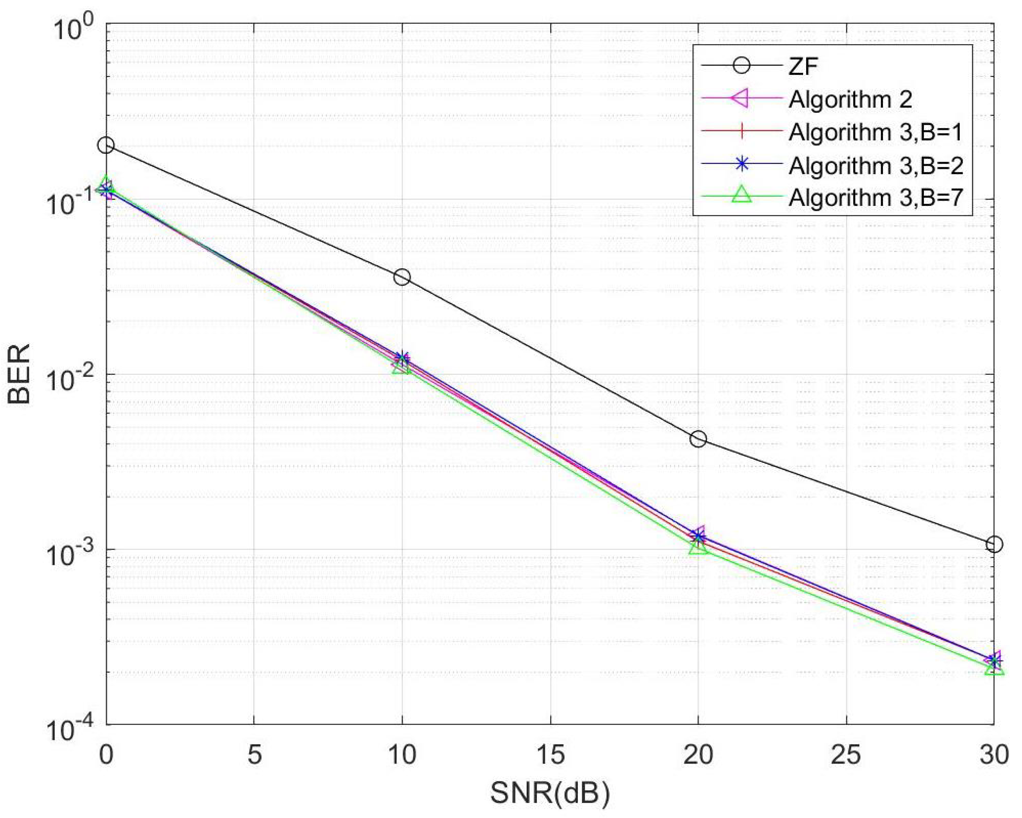
5. Simulation Results and Discussions

We evaluate the performance of the proposed Algorithms 2 and 3 through simulations and discuss implications of symbol number B in one subframe on the performance of Algorithm 3. In addition, we compare the BER of the proposed algorithms with that of the traditional ZF detection.

In the simulation, we use the MIMO-OFDM system parameters set as shown in

Table 3. Simulation parameters.

Simulation Parameter Table
Transmit Antennas $N_t$	4
Receive Antennas $N_r$	4
Subcarriers K	64
Data Frame Length $N_f$	14
Doppler Shift/Hz	400
Sampling Rate/MHz	30.72

. We conduct simulations in a MIMO-OFDM system with $N_t=4$ transmit antennas, $N_r=4$ receive antennas, $K=64$ subcarriers, and a data frame length of $N_f=14$. The channel model we employ is a time-frequency variation TDL-B channel with 12 taps [17], a Doppler shift of 400 Hz, and a sampling rate of 30.72 MHz. Under such channel conditions, Algorithm 1 cannot be applied.

Figure 2 shows the BER of proposed algorithms with different number of symbols B of 1, 2, and 7 under QPSK modulation. The performance of the conventional ZF detection is also shown in the figure for comparison. From Figure 2, we can see that the BER values decrease for all algorithms as SNR increases. The performance of Algorithm 3 is significantly better than direct ZF detection. When BER is ${10}^{-2}$, Algorithm 3 with $B=1$ has an approximately 5dB SNR gain compared to the direct ZF detection algorithm. The simulation also shows the performances of Algorithm 3 with $B=1$ and $B=2$ are relatively similar and Algorithm 3 with $B=7$ performs better under high-SNR conditions. However, according to the discussion in Section 4.2, there is a significant difference in the complexity of Algorithm 3 with different B values. The smaller the number of symbols B, the lower the complexity. The complexity of Algorithm 3 is approximately $\mathrm{O}(2.8\times {10}^{10})$ when $\mathit{B}=1$, $\mathrm{O}(11.3\times {10}^{10})$ when $\mathit{B}=2$, and $\mathrm{O}(138.1\times {10}^{10})$ when $\mathit{B}=7$. By comparing the performances of Algorithms 2 and 3, it can be noted that the BER performance of Algorithm 3 with the number of symbols of 1 and Algorithm 2 is similar. However, the complexity of Algorithm 3 with $B=1$ is $0.73\%$ of Algorithm 2. Therefore, in practical applications, using Algorithm 3 with $B=1$ can achieve both superior performance and lower computational complexity.

We also investigate the BER performance of the algorithms under different signal modulation schemes. Keeping the antennas, carriers, and data frame length the same as the previous settings, we focused on the case where the number of symbols is 1 and examined the performance when the signal modulation scheme is changed.

Figure 3 shows the BER of the proposed Algorithm 2, Algorithm 3 with a different number of symbols B, and the direct ZF detection algorithm under BPSK modulation. From Figure 3, it is easy to observe that Algorithm 3 is superior to that of the direct ZF detection algorithm, with an SNR gain of approximately 6dB when the BER is ${10}^{-2}$. This shows that Algorithm 3 performs well in the case of various modulation schemes. The results also indicate that the performance of Algorithm 3 with different subframe lengths is basically similar, except that with $B=7$ it improves slightly under high SNR. However, the higher the value of B, the higher the computational complexity of Algorithm 3. Comparing the BER performance of Algorithms 2 and 3, the performance of Algorithm 2 is similar to that of Algorithm 3 with $B=1$. Similarly to the case of QPSK modulation, the complexity of Algorithm 3 is lower than Algorithm 2. These simulations show that Algorithm 3 is effective in different modulation scenarios, and the utilization of subframe and pilots for signal estimation in Algorithm 3 contributes to BER performance and computational complexity improvement.

6. Conclusions

In this paper, we propose a time-varying channel manifold optimization algorithm for MIMO-OFDM systems, which enables efficient signal detection with low complexity. The proposed algorithm utilizes manifold optimization techniques to optimize the signals for MIMO-OFDM systems and involves the following steps. First, the estimated channel obtained from a GAN-based method is used for ZF detection to obtain the initial estimated signals. Subsequently, the optimization problem is solved by dividing the signals into subframes and the pilot part of the signals is used as a criterion to determine the completion of the optimization process. The simulation results show that Algorithm 3 has superior performance compared to direct ZF detection. When the BER is ${10}^{-2}$, Algorithm 3 with $B=1$ has an approximately 5 dB SNR gain compared to the direct ZF detection algorithm under QPSK modulation. Furthermore, the algorithm achieves a reduced bit error rate while maintaining low computational complexity.

References

1. Rusek, F.; Persson, D.; Lau, B.K.; Larsson, E.G.; Marzetta, T.L.; Edfors, O.; Tufvesson, F. Scaling Up MIMO: Opportunities and Challenges with Very Large Arrays. IEEE Signal Process. Mag. 2013, 30, 40–60. [Google Scholar] [CrossRef]
2. Andrews, J.G.; Buzzi, S.; Choi, W.; Hanly, S.V.; Lozano, A.; Soong, A.C.K.; Zhang, J.C. What Will 5G Be? IEEE J. Sel. Areas Commun. 2014, 32, 1065–1082. [Google Scholar] [CrossRef]
3. Farzamnia, A.; Moung, E.; Hlaing, N.W.; Kong, L.E.; Haldar, M.K.; Fan, L.C. Analysis of MIMO System through Zero Forcing and Minimum Mean Square Error Detection Scheme. In Proceedings of the 2018 9th IEEE Control and System Graduate Research Colloquium (ICSGRC), Shah Alam, Malaysia, 3–4 August 2018; pp. 172–176. [Google Scholar] [CrossRef]
4. Zhang, B.; Yu, J.L.; Lai, J.W. A fast subspace channel estimation for STBC-based MIMO-OFDM systems. In Proceedings of the 2014 11th International Symposium on Wireless Communications Systems (ISWCS), Barcelona, Spain, 26–29 August 2014; pp. 75–79. [Google Scholar] [CrossRef]
5. Scherb, A.; Zheng, C.; Kuhn, V.; Kammeyer, K. Comparison of methods for iterative joint data detection and channel estimation. In Proceedings of the 2004 IEEE 59th Vehicular Technology Conference, VTC 2004-Spring (IEEE Cat. No.04CH37514). Milan, Italy, 17–19 May 2004; Volume 1, pp. 98–102. [Google Scholar] [CrossRef]
6. Zhou, Y.; Ng, T.S. Performance analysis on MIMO-OFCDM systems with multi-code transmission. IEEE Trans. Wirel. Commun. 2009, 8, 4426–4433. [Google Scholar] [CrossRef]
7. Zhou, Y.; Ng, T.S. MIMO-OFCDM systems with joint iterative detection and optimal power allocation. IEEE Trans. Wirel. Commun. 2008, 7, 5504–5516. [Google Scholar] [CrossRef]
8. Zhong, K.; Wu, Y.C.; Li, S. Signal Detection for OFDM-Based Virtual MIMO Systems under Unknown Doubly Selective Channels, Multiple Interferences and Phase Noises. IEEE Trans. Wirel. Commun. 2013, 12, 5309–5321. [Google Scholar] [CrossRef]
9. Hu, J.; Liu, X.; Wen, Z.; Yuan, Y.X. A Brief Introduction to Manifold Optimization. J. Oper. Res. Soc. China 2020, 8, 199–248. [Google Scholar] [CrossRef]
10. Cao, Y.; Yin, H.; He, G.; Debbah, M. Manifold Learning-Based CSI Feedback in Massive MIMO Systems. In Proceedings of the ICC 2022—IEEE International Conference on Communications, Seoul, Republic of Korea, 16–20 May 2022; pp. 225–230. [Google Scholar] [CrossRef]
11. Chen, J.C. Manifold Optimization Approach for Data Detection in Massive Multiuser MIMO Systems. IEEE Trans. Veh. Technol. 2018, 67, 3652–3657. [Google Scholar] [CrossRef]
12. Hong, X.; Gao, J.; Chen, S. Semi-Blind Joint Channel Estimation and Data Detection on Sphere Manifold for MIMO with high-order QAM Signaling. J. Frankl. Inst. 2020, 357, 5680–5697. [Google Scholar] [CrossRef]
13. Yu, X.; Tu, L.; Yang, Q.; Yu, M.; Xiao, Z.; Zhu, Y. Hybrid Beamforming in mmWave Massive MIMO for IoV With Dual-Functional Radar Communication. IEEE Trans. Veh. Technol. 2023, 72, 9017–9030. [Google Scholar] [CrossRef]
14. Li, Z.; Wang, S.; Wen, M.; Wu, Y.C. Secure Multicast Energy-Efficiency Maximization With Massive RISs and Uncertain CSI: First-Order Algorithms and Convergence Analysis. IEEE Trans. Wirel. Commun. 2022, 21, 6818–6833. [Google Scholar] [CrossRef]
15. Absil, P.A.; Mahony, R.; Sepulchre, R. Optimization Algorithms on Matrix Manifolds; Princeton University Press: Princeton, NJ, USA, 2008; Volume 78. [Google Scholar] [CrossRef]
16. Boumal, N.; Mishra, B.; Absil, P.A.; Sepulchre, R. Manopt, a matlab toolbox for optimization on manifolds. J. Mach. Learn. Res. 2014, 15, 1455–1459. [Google Scholar]
17. Gong, C.; Hu, D. A GAN-Based Channel Estimation Method for MIMO OFDM Systems. In Proceedings of the 2023 8th International Conference on Communication, Image and Signal Processing (CCISP), Chengdu, China, 17–19 November 2023. [Google Scholar]
18. Zhang, B.; Hu, D.; Wu, J.; Xu, Y. An Effective Generative Model Based Channel Estimation Method With Reduced Overhead. IEEE Trans. Veh. Technol. 2022, 71, 8414–8423. [Google Scholar] [CrossRef]
Figure 1. Flow diagram of Algorithm 3.
Electronics 13 02555 g001
Figure 2. BER vs. SNR under QPSK modulation.
Electronics 13 02555 g002
Figure 3. BER vs. SNR under BPSK modulation.
Electronics 13 02555 g003