Abstract
This paper focuses on the influence of the fractional-order (FO) resonant capacitor on the zero-voltage-switching quasi-resonant converter (ZVS QRC). The FO impedance model of the capacitor is introduced to the circuit model of the ZVS QRC; hence, a piecewise smooth FO model is developed for the converter. Numerical solutions of the converter are obtained by using both the fractional Adams–Bashforth–Moulton (F-ABM) method and Oustaloup’s rational approximation method. In addition, the analytical solution of the converter is obtained by the Grünwald–Letnikov (GL) definition, which reveals the influence of the FO resonant capacitor on the zero-crossing point (ZCP) and resonant state of the converter. An experimental platform was built to verify the results of the theoretical analysis and numerical calculation.
1. Introduction
Soft-switching techniques are widely used in power converters to reduce switching losses and lift system efficiency [1,2]. A variety of soft-switching schemes based on high-frequency resonant impedance networks have been proposed one after the other, such as the zero-voltage-switching (ZVS) and zero-current-switching (ZCS) techniques, to name but a few [3,4,5]. It is generally accepted that the parameter configuration of passive components is of great importance for the design of different types of high-frequency resonant networks that can be used for soft switching [6,7,8].
The resonant converter can achieve ZVS with the assistance of capacitors [9,10]. For this kind of converters that contains the LC resonant tank, capacitors, as a vital part of the LC resonant tank, usually play a pivotal role in the process of realizing resonance. However, there is a common phenomenon of parameter drift in capacitors. For example, in the literature [11,12], one can find that the capacitance and equivalent series resistance (ESR) of the capacitor considerably changes with the temperature, aging, frequency, and component tolerance. Specifically, electrolyte evaporation, oxide layer deterioration for electrolytic capacitors, and the excessive self-healing for metalized polypropylene film (MPPF) capacitors are also the reasons for the parameter drift of the capacitor [13,14]. In most existing works, the parameter drift characteristics of capacitors have been widely studied, and different kinds of integer-order (IO) impedance models have been proposed. The characteristic analysis of resonant converters relies on traditional integer-order lumped-parameter models, and their time domain solutions depend on solving the initial-value problem of IO differential equations. However, with the ever-deepening research, the topology of the models becomes increasingly complex, as those surveyed in the literature [15,16,17]. In addition, IO impedance models usually cannot effectively reflect the correlation between the microscopic characteristics of the electronic components, the parameter drift of the component parameters, and the performance of the converters [18,19]. As a result, the analysis of the errors will be introduced to the design of the resonant converters, thereby affecting the working performance of circuit systems [20,21,22,23].
In recent years, researchers have discovered the presence of fractional-order phenomena in fields such as mechanics, physical engineering, and materials science [24]. Existing studies indicate that fractional-order models can more accurately reflect the physical phenomena of actual systems [25]. Especially in the field of circuits, the fractional-order characteristics of electronic components have been revealed. For example, the literature [26] uncovers the FO characteristic of MOSFETs’ interelectrode capacitance. The literature [27] reveals the FO characteristics of the capacitors by exploring the electrochemical principles of aluminum electrolytic capacitors. The literature [28] investigates a new implementation of a passive FO capacitor based on a single-component FO inductor, which truly reflects the infinite-dimensional nature of the fractional-order impedance characteristic. The memristor is also a nonlinear device with memory characteristics [29]. On the basis of the aforementioned studies, scholars have conducted modeling and analysis research on fractional-order converters [30,31,32].
On the other hand, due to the existence of switching devices, the FO models for DC–DC converters have been established, such as FO Buck, Boost, Buck–Boost, and Flyback converters, which exhibit strong nonlinear characteristics [33,34,35]. These models not only improve modeling accuracy, but also accurately describe the true dynamic behavior of the converters, providing a more precise theoretical basis for optimizing converter control. However, most of the research focuses primarily on the modeling and analysis of fractional-order converters with the lower orders and lacks characteristic analysis from the time domain perspective.
For the ZVS QRC, a kind of circuit system that relies on resonant operating points for circuit design, the influence of the fractional characteristics of the capacitance on circuit performance is awaiting study. Accordingly, the contents and contributions of this paper include the following points:
- 1.
- In order to reveal the influence of factional-order (FO) resonant capacitors on the ZVS QRC, this work develops an FO piecewise-smooth model for the converter, which contains the FO impedance model of the resonant capacitor.
- 2.
- The time domain resonant characteristics of the converter are analyzed by using the proposed FO piecewise-smooth model. Time domain analytical solutions of the converter are calculated by using the Grünwald–Letnikov (GL) definition of fractional calculus. In addition, numerical solutions are also obtained for comparison and validation, where the fractional Adams–Bashforth–Moulton (F-ABM) method and Oustaloup’s rational approximation method are used.
- 3.
- Both circuit-level simulation and an experimental platform are built to verify the theoretical analysis and numerical calculations. Compared with the IO-based approach, the accuracy of the FO-model-based analysis is improved, and some of the resonant performances of the converter, such as the zero-voltage crossing time and voltage ripples, can be revealed in a more accurate way.
The remainder of the paper is organized as follows: Section 2 introduces the relationship between the FO characteristics of the resonant capacitor and the switching modes of the converter through an FO piecewise-smooth model. Section 3 solves the initial-value problem of fractional differential equations, and the the quantitative relationship among resonant conditions, the zero-crossing voltage, and the FO of the resonant capacitor are obtained. In Section 4, both the simulation and experimental results are given for the validation of the theoretical analysis and numerical calculations via the F-ABM method and GL definition. Section 5 gives the conclusion.
2. Circuit Analysis Framework Based on Fractional-Order Piecewise-Smooth Model
Figure 1 shows a typical ZVS QRC, in which a resonant capacitor is in parallel with the power switch and the power diode . Therefore, the charging or discharging state of the resonant capacitor changes with the on or off state of the switch , thus affecting the resonant state of the resonant unit and the switching mode of the converter. Note that the resonant capacitor is modeled by a simplified fractional-order impedance model, which comprises an ideal fractional-order capacitor and a series resistance [27]. Then, the switching mode and working states of the converter can be deduced according to the KVL law and the KCL law.
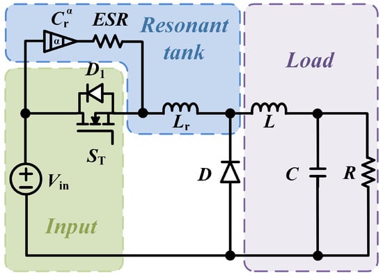
Figure 1.
ZVS QRC with a fractional-order resonant capacitor.
2.1. Switching Mode Analysis
The schematic in Figure 1 can provide the adjustment of the resonant frequency by ensuring zero-voltage-switching conditions, i.e., the voltage or must be zero whenever the switch is closed, as per the waveforms in Figure 2. In one steady-state switching period, the converter experiences six switching modes, the equivalent circuits of which are depicted in Figure 3.
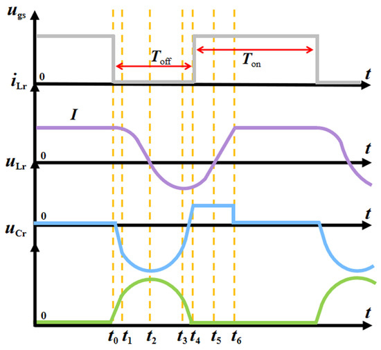
Figure 2.
Ideal waveforms of the ZVS QRC with a fractional-order resonant capacitor. is the gate-source voltage of MOSFET, is the current of the resonant inductor , is the voltage of the resonant inductor , and is the voltage of the resonant capacitor .
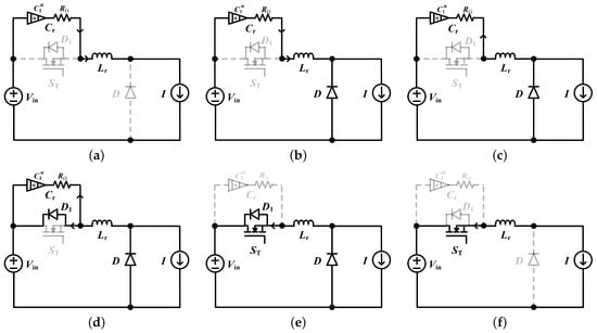
Figure 3.
Operation topology of the ZVS-QRC with a fractional-order resonant capacitor: (a) mode 1, (b) mode 2, (c) mode 3, (d) mode 4, (e) mode 5, and (f) mode 6.
- 1.
- Mode 1 (): In this time period, is turned off, and the resonant capacitor is charged by and L. The voltage increases until the voltage become zero and the voltage reaches the input voltage ; thus, the converter in this period can be governed by:where is the nominal capacitance of the resonant capacitor , is the fractional order, I is the current of inductor L.
- 2.
- Mode 2 (): In this time period, the resonant capacitor is charged by , diode D is in conduction state, and , , and form a resonant unit. While the current continues to decrease, the voltage continues to rise. At time , reaches its peak value. Due to the voltage rising from the initial value to the peak value of the resonance progress, the duration of this mode is a quarter cycle and is determined by:in which is the inductance of the resonant inductor and is the resonant angle frequency.
- 3.
- Mode 3 (): In this time period, the resonant inductor and the resonant capacitor charge and discharge each other. The current changes direction. The decrease of the voltage leads the voltage to increase to zero. At time , equals and reaches its reverse resonant peak. The duration of this mode is analyzed similarly to mode 2, and it is given by:
- 4.
- Mode 4 (): The resonant capacitor is reversely charged by the resonant inductor , and the voltage continues to decrease. When decreases to zero, this mode ends.The converter in the resonant process of to can be governed by:where is the input voltage and is the voltage of .
- 5.
- Mode 5 (): In this time period, the diode conducts and the voltage is clamped to zero. The voltage of resonant inductor is constant and equal to , and the current linearly decays to zero at time ; the converter in this mode can be described by:
- 6.
- Mode 6 (): The switch is turned on. At time , resonant inductor current equals I, and diode D is turned off.
The variations of the times and versus the fractional-order of the resonant capacitor have a similar trend, which is give in Figure 4:
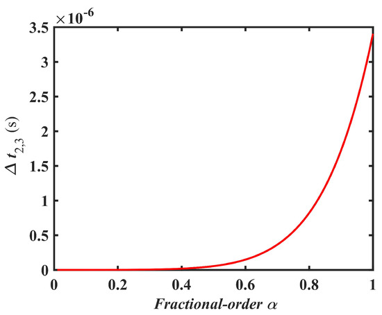
Figure 4.
Variation trend of and with the fractional-order .
Based on the above, one can find that the ZVS QRC with a fractional-order resonant capacitor can be governed by piecewise-smooth fractional-order models. In order to reveal it’s resonant characteristics, it is essential to calculate the fractional differential Equation (4), so that the initial-value problem of the fractional-order differential equation arises.
2.2. Computation Approaches
2.2.1. Solutions Obtained by F-ABM Method
For any nonlinear dynamical system with initial values, the fractional-order differential equation describing its dynamics is:
where , .
The integral equation describing this nonlinear dynamical system is:
Based on the above definition of F-ABM, let . The fractional differential equations in Equations (1) and (4) can be written in the following discrete form [36]:
where n is any integer, and the correction coefficient is
The flow chart of the F-ABM method is shown in Figure 5:
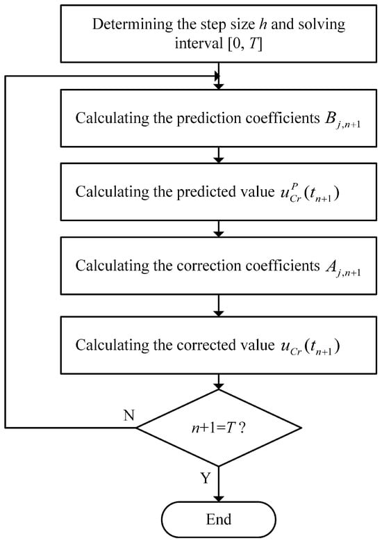
Figure 5.
A flow chart of the F-ABM method.
2.2.2. Solutions Obtained by Oustaloup’s Rational Approximation Method
The ideal fractional-order derivation and differential can be approximated by a pre-designed rational fraction [37]:
where K is the pre-designed gain parameter and the number N of pole-zero doublets is determined by the pre-determined amplitude–frequency characteristic error and the pre-designed frequency range:
in which , , , , MHz, and y is the pre-determined error.
The expression for the zeros and poles can be obtained through inductive recursion relationships:
The rational fraction in Equation (13) is partially expanded and transformed into the following transfer function:
The parameter and can be obtained by the transform-obtained zero-pole representation in a rational fraction form using the and functions. The meaning of the first function is transforming the parameters of the zero-pole filter into the form of the transfer function, and the meaning of the second function is the partial fraction expansion. The values of and in the impedance approximation circuit are calculated by using the following formula:
A simplified fractional-order capacitor model is introduced in the ZVS QRC. , and . The capacitance value, ESR, and impedance modulus of the fractional-order resonant capacitor are measured by a high-precision LCR meter in Figure 6, and the fractional-order of the capacitor is predicted by the method in the previous work [27], which can be verified by the impedance–frequency curve and resistance–frequency curve shown in Figure 7. By data fitting, we found that the fractional-order of this resonant capacitor is around 0.987.
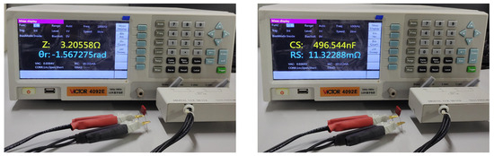
Figure 6.
A glimpse of the capacitor test scenarios.
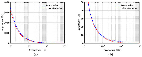
Figure 7.
Comparison between test data and the prediction results of the fractional-order impedance model: (a) frequency–impedance curve and (b) frequency–resistance curve.
The above results indicate that the CBB film capacitor has fractional-order characteristics. However, there are no such components in existing simulation software. Therefore, we used Oustaloup’s approximation method to build such a fractional-order capacitor in the simulation for comparison, the structure of which is shown in Figure 8. An ideal fractional-order capacitor can be obtained by connecting the resistor and the capacitor in parallel as a unit in series, which is verified by the amplitude frequency characteristic and the phase frequency characteristic in Figure 9. Obviously, the frequency range for this approximation is from Hz to Hz and the pre-determined error y is less than 3 dB. The resistors and in Table 1 are the components involved in the capacitor and resistor parallel units in the method.
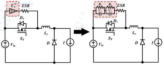
Figure 8.
An ideal fractional-order capacitor approximated by Oustaloup’s method.
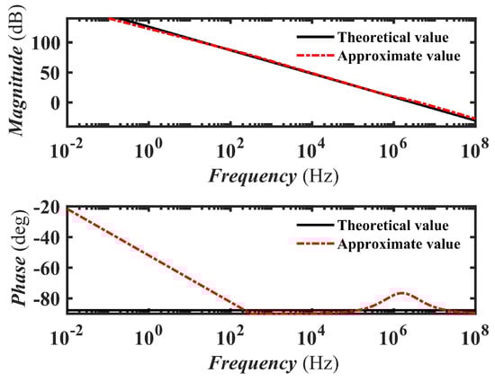
Figure 9.
Bode diagrams of ideal order-0.987 capacitor and its rational approximation circuit.

Table 1.
The fractional-order capacitor parameters.
3. Resonant State Analysis
3.1. Analytical Solutions Obtained by GL Definition
The GL definition method provides a theoretical solution to the resonance equation system, and it serves as a reference in comparison with the F-ABM and Oustaloup numerical methods mentioned above. The GL definition of the FO derivative of function is obtained [38]:
where is the fractional-order calculus operator, t is an independent variable, h is the step size, the superscript GL represents to the Grünwald–Letnikov definition, and is the binomial coefficient, which can be obtained by the recurrence formula:
By the GL definition, the time domain expressions of Equation (4) are transformed into:
in which the fractional-order equals 0.987, is the inductance of the resonant inductor, is the capacitance of the resonant capacitor, and is the resistance of the resonant capacitor shown in Figure 1. is the starting point of the resonant progress shown in Figure 2.
By solving Equations (18) and (20), the voltage and current of the resonance process () are obtained:
Let Equation (21) equal zero; one can obtain the analytical expressions of the ZCP. In addition, one can obtain the analytical expressions of the peak and valley values of the state variables. It can be seen that the order of the resonant capacitance is explicitly included in these equations. Therefore, the above analytical expressions can be directly used to analyze the influence of fractional order on the resonant state of the ZVS QRC.
The results of the numerical solution for the ZVS QRC based on the F-ABM method, Oustaloup’s method, and the GL definition method are obtained as shown in Figure 10. It can be observed that the waveforms obtained by the three approaches coincide with each other. Therefore, the results of the numerical calculation and simulation by these three methods can be used as a reference for the theoretical analysis.
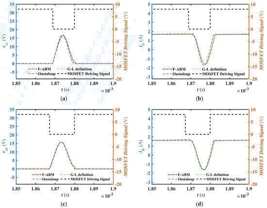
Figure 10.
Comparison of the ZVS QRC: (a) resonant capacitor voltage at , (b) resonant inductor current at , (c) resonant capacitor voltage at , and (d) resonant inductor current at .
3.2. Influence of the Fractional-Order Resonant Capacitor
According to the above theoretical analysis, the state variables of the ZVS QRC with different orders of the resonant capacitor can be obtained, as shown in Figure 11.

Figure 11.
Influence on resonant capacitor voltage of different fractional orders.
To more specifically show the data changes in Figure 11, a summary of the ZCP and the peak resonant voltage change with the order is given in Table 2. It can be seen that, with the decrease of the order , the peak resonant voltage is obviously increased, and the ZCP shows a shortening trend.
Table 2.
Peak value and ZCP at different orders .
The resonant progress of ZVS QRC is shown in Figure 3b,c, and its resonant unit is a fractional-order RLC series circuit as given in Figure 12. The impedance Z of this fractional-order RLC series circuit is given by:
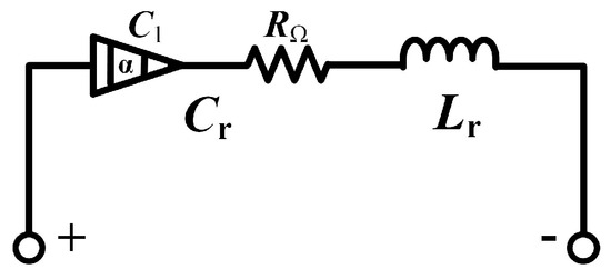
Figure 12.
A fractional-order RLC series circuit.
By Euler’s formulation, the impedance Z of the fractional-order RLC series circuit can be rewritten as:
Let the imaginary part in Equation (23) equal zero; the resonant angle frequency is described by:
In can be seen in Equation (24) that the resonant angle frequency of the converter is highly dependent on the values of its resonant elements. Tolerances in these components can lead to variations in the actual resonant frequency from its designed value. This shift can reduce the efficiency of the energy transfer within the circuit. The influence on resonant angle frequency of different FO αs is shown in Figure 13. It can be seen that, with the increase of , the resonant angle frequency increases first and then decreases; when equals 0.05, it reaches the peak value.
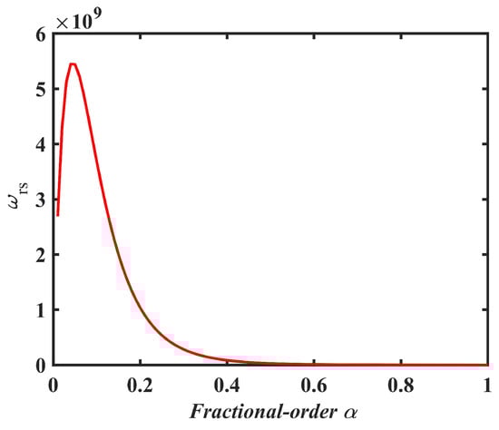
Figure 13.
Influence on resonant angle frequency of different fractional-order .
The quality factor (Q-factor) of a resonant circuit, which indicates its bandwidth and energy loss characteristics, can be affected by the tolerances of the resonant elements. A higher tolerance can lead to a lower Q-factor, implying greater energy dissipation and a broader resonance peak, potentially affecting the circuit’s selectivity and performance. In this manuscript, the Q-factor of a ZVS-QRC with an order- resonant capacitor is:
The power losses caused by the resonant capacitor are usually determined by its ESR [39], that is:
where is the RMS value of the current through the resonant capacitor and ESR is the equivalent series resistance of the resonant capacitor. According to the FO equivalent impedance model of the resonant capacitor, the value of the ESR is:
It can be seen that the ESR of the FO capacitor model not only includes the IO capacitor model , but is also related to the order . By changing the order , one can obtain the variation trend of the power losses of resonant capacitor with the order , as depicted in Figure 14. This validates the fractional-order characteristics present in actual capacitors and reveals the limitations of IO capacitor models.
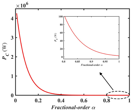
Figure 14.
The variation trend of versus the FO .
4. Validation and Discussion
4.1. Experiment Configuration
Experiments were carried out to validate the theoretical analysis and calculation results. The experiment configurations are depicted in Table 3, and a glimpse of the test scene is depicted in Figure 15, while the design process of the parameters was as follows:
Table 3.
Parameter configuration in the experiments.
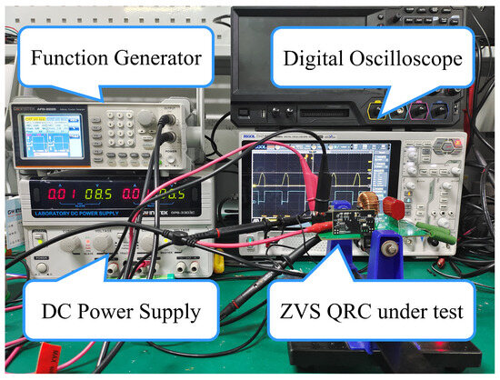
Figure 15.
A glimpse of the experiment scene.
Step 1: According to the simple parameter expression obtained in the ZVS QRC model with an ideal resonant capacitor, the approximate range of , , L, C, R, D, , and can be determined.
Step 2: The C, R, Z, and of the capacitor are collected by the LCR meter in Figure 6 from low frequency to high frequency, then the parameters of the simplified FO capacitor are identified by the differential evolution method.
Step 3: Construct an FO capacitor with order by Oustaloup’s rational approximation method as shown in Figure 8.
Step 4: Verify the accuracy and effectiveness of the design methodology presented in the PSIM simulation and experiments.
4.2. Practical Implications
This work actually constructs a bridge between the microscopic characteristics of capacitors, the variation law of capacitor parameters, and the working characteristics of resonant converters by introducing the method of fractional calculus. The findings of this work have the following possible practical implications:
- 1.
- Power conversion efficiency: By using FO-based modeling and analysis approaches, more accurate analyzing results can be obtained, thus benefiting the parameter design and component selection of circuit systems that contain components with fractional-order characteristics. From the research in this article, it can be seen that the working state of ZVS QRCs is closely related to the FO characteristics of the resonant capacitor. Accordingly, the authors intend to analyze the power conversion efficiency of ZVS QRCs and its relationship with the FO characteristics of resonant capacitors in future works.
- 2.
- Controller design and optimization: The FO characteristics of resonant capacitors of course have effects on the frequency domain characteristics of circuit systems. Therefore, when designing controllers for such converters in the future, it is also necessary to study the relationship between the FO characteristics of resonant capacitors and the frequency domain characteristics of ZVS QRCs. The FO piecewise-smooth model established in this work can be further transformed into the s domain by the Laplace transform for research in the aforementioned fields.
Therefore, it is necessary to promote the application of FO-related methods in a vast variety of practical applications, such as electric vehicle applications, where various electrochemical components are used and FO characteristics are commonly present. But, the main challenges are as follows:
- 1.
- The universality of FO parameter characteristics: Actual electronic devices’ parameters are often influenced by environmental conditions, manufacturing variances, and operational circumstances. This work only tested a batch of CBB film capacitors under constant temperature and working conditions. It remains to be studied whether CBB capacitors manufactured by other manufacturers still have the same FO parameter characteristics under more complex working conditions.
- 2.
- Computational demands: One can find that both the analyzed solutions and numerical solutions of an FO converter are in complicated iterative forms. Therefore, by using FO models in design and analysis, the computational cost will be increased to some extent.
To overcome these challenges, we plan to conduct more extensive testing scenarios in future works, testing CBB capacitors from different manufacturers, verifying whether they have a unified parameter variation pattern, and establishing a universal model.
4.3. Performance Analysis and Comparison
The experiment waveforms are give in Figure 16 and Figure 17. One can find that the experiment waveforms of the ZVS QRC are similar to the simulation results with fractional-order resonant capacitors.
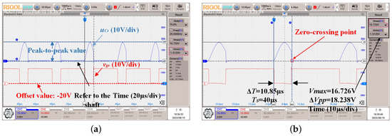
Figure 16.
Experimental waveforms of : (a) Time = 20 μs/div; (b) Time = 10 μs/div.
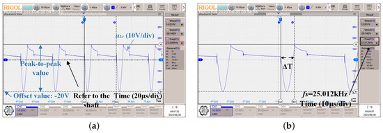
Figure 17.
Experimental waveforms of : (a) Time = 20 μs/div; (b) Time = 10 μs/div.
It can be seen from Figure 16 and Figure 17 that the theoretical calculation and simulation results shown in Figure 10 coincide with the experimental waveforms. In Figure 17, the blue solid lines are the voltage of the resonant capacitor and the red solid lines show the MOSFET driving signal . After conducting a thorough analysis and evaluation based on several key performance indicators (KPIs) of the resonant converter, such as the zero-crossing point (ZCP) and peak voltage (PV), we have determined that Oustaloup’s method offers better performance and optimization for the specific application and conditions outlined in our study. In order to explore the influence of the FO resonant capacitors, Table 4 and Table 5 list the peak resonant voltage and ZCP obtained by different methods for comparison and verification for an FO equal to 0.987 and equal to 1. One can find that Oustaloup’s method represents the PV and ZCP of the resonant capacitor error generally within 2% and the F-ABM method represents the PV of the resonant capacitor error generally within 2%, while the FO model in calculating the ZCP error is within 9%, which is less than the error of the ideal IO capacitor model including parasitic parameters. It is proven that the FO has a better fitting effect than the ideal IO capacitor model.
Table 4.
Comparisons of PV between FO, IO values, and experiments.
Table 5.
Comparisons of ZCP between FO, IO values, and experiments.
5. Conclusions
The FO characteristics of capacitors have been widely confirmed in existing works. In order to reveal the influence of factional-order resonant capacitors on ZVS QRCs, this work develops an FO piecewise-smooth model for the converter, which contains the FO impedance model of the resonant capacitor. To analyze the resonant characteristics of the converter, numerical solutions based on the F-ABM method and Oustaloup’s rational approximation method were calculated, and analytical solutions were also deduced based on the GL definition. With the decrease of the order , the peak resonant voltage obviously increased, and the ZCP showed a shortening trend. The experimental data showed that the F-ABM method is more accurate in describing the PV of a resonant capacitor, Oustaloup’s method has more advantages in calculating the ZCP and PV, and the FO capacitor model can reflect the real working conditions of the capacitor more exactly, which further confirms the fractional-order characteristics of the capacitor. Compared with the IO-based approach, the accuracy of the time domain analysis can be improved, and some microscopic phenomena of resonant converters can be better explained by using the modeling and calculation methods based on the fractional calculus. However, the fractional calculus-related theory and computing methods are still developing, and the universality and ease of use of methods still need to be widely verified.
Author Contributions
Conceptualization, methodology, software, formal analysis, resources, writing—review and editing, and supervision, X.C.; writing—original draft preparation, validation, and data curation, W.C. All authors have read and agreed to the published version of the manuscript.
Funding
This research received no external funding.
Data Availability Statement
The data are contained within the article.
Conflicts of Interest
The authors declare no conflicts of interest.
References
- Kazimierczuk, M.K.; Dariusz, C. Resonant Power Converters: Quasi Resonant and Multi Resonant DC-DC Power Coverters; Wiley: Hoboken, NJ, USA, 2012; pp. 485–509. [Google Scholar]
- Chen, Y.; Xu, D. Review of Soft-Switching Topologies for Single-Phase Photovoltaic Inverters. IEEE Trans. Power Electron. 2022, 37, 1926–1944. [Google Scholar] [CrossRef]
- Mohammed, S.; Jung, J. A State-of-the-Art Review on Soft-Switching Techniques for DC-DC, DC-AC, AC-DC, and AC-AC Power Converters. IEEE Trans. Ind. Inform. 2021, 17, 6569–6582. [Google Scholar] [CrossRef]
- Zhu, B.; Yang, Y.; Wang, K.; Liu, J. Vilathgamuwa, D. High Transformer Utilization Ratio and High Voltage Conversion Gain Flyback Converter for Photovoltaic Application. IEEE Trans. Ind. Appl. 2024, 60, 2840–2851. [Google Scholar] [CrossRef]
- Kazimierczuk, M.; Jozwik, J. Resonant DC/DC converter with class-E inverter and class-E rectifier. IEEE Trans. Ind. Electron. 1989, 36, 468–478. [Google Scholar] [CrossRef]
- Feng, J.; Li, Q.; Lee, F.; Fu, M. LCCL-LC Resonant Converter and Its Soft Switching Realization for Omnidirectional Wireless Power Transfer Systems. IEEE Trans. Power Electron. 2021, 36, 3828–3839. [Google Scholar] [CrossRef]
- Luo, H. Voltage-Mode Variable-Frequency Controlled LLC Resonant Power Factor Correction Converter and Its Accurate Numerical Calculation Analysis. IEEE J. Emerg. Sel. Top. Power Electron. 2023, 11, 1979–1994. [Google Scholar] [CrossRef]
- Xu, J.; Sun, Y.; Xu, G.; Su, M. Coupled Inductor Based Bidirectional Resonant Converter with Sine Wave Modulation in Wide Voltage Range. IEEE Trans. Power Electron. 2022, 37, 3713–3718. [Google Scholar] [CrossRef]
- Lee, K.; Ha, J. Resonant Switching Cell Model for High-Frequency Single-Ended Resonant Converters. IEEE Trans. Power Electron. 2019, 34, 11897–11911. [Google Scholar] [CrossRef]
- Askari, S.; Farzanehfard, H. Highly Efficient Nonisolated Constant Output Current LCC Resonant Converter with Wide Input Voltage Range. IEEE Trans. Power Electron. 2023, 38, 10052–10059. [Google Scholar] [CrossRef]
- Amaral, A.; Cardoso, A. Simple experimental techniques to characterize capacitors in a wide range of frequencies and temperatures. IEEE Trans. Instrum. Meas. 2010, 59, 1258–1267. [Google Scholar] [CrossRef]
- Lai, Y.; Yu, M. Online Autotuning Technique of Switching Frequency for Resonant Converter Considering Resonant Components Tolerance and Variation. IEEE J. Emerg. Sel. Top. Power Electron. 2018, 6, 2315–2324. [Google Scholar] [CrossRef]
- Vishay, R. Film Capacitors General Technical Information. 2018. Available online: https://www.tdk-electronics.tdk.com/download/530754/480aeb04c789e45ef5bb9681513474ba/pdf-generaltechnicalinformation.pdf (accessed on 15 April 2022).
- Pong, M.; Pang, H. Power Converter Remaining Life Estimation. U.S. Patent US8412486B2, 2 April 2013. [Google Scholar]
- Braham, A.; Lahyani, A.; Venet, P.; Rejeb, N. Recent Developments in Fault Detection and Power Loss Estimation of Electrolytic Capacitors. IEEE Trans. Power Electron. 2010, 25, 33–43. [Google Scholar] [CrossRef]
- Amaral, A.; Cardoso, A. On-line fault detection of aluminium electrolytic capacitors, in step-down DC-DC converters, using input current and output voltage ripple. IET Power Electron. 2012, 3, 315–322. [Google Scholar] [CrossRef]
- Parler, S. Improved Spice models of aluminum electrolytic capacitors for inverter applications. IEEE Trans. Ind. Appl. 2003, 39, 929–935. [Google Scholar] [CrossRef]
- Zhou, S.; Tang, J.; Zeng, Q. A novel high frequency isolated dual-transformer LCL-type resonant AC/DC converter to minimize total loss over whole load range. IEICE Electron. Express 2024, 21, 20240086. [Google Scholar] [CrossRef]
- Lee, Y.L.; Hwu, K.I. Multiphase LLC DC-Link Converter with Current Equalization Based on CM Voltage-Controlled Capacitor. Energies 2024, 17, 2793. [Google Scholar] [CrossRef]
- Xu, J.; Gu, L.; Rivas-Davila, J. Effect of Class 2 Ceramic Capacitor Variations on Switched-Capacitor and Resonant Switched-Capacitor Converters. IEEE J. Emerg. Sel. Top. Power Electron. 2020, 8, 2268–2275. [Google Scholar] [CrossRef]
- Mustafa, Y.; Subburaj, V.; Ruderman, A. Revisited SCC Equivalent Resistance High-Frequency Limit Accounting for Stray Inductance Effect. IEEE J. Emerg. Sel. Top. Power Electron. 2021, 9, 638–646. [Google Scholar] [CrossRef]
- Zhang, Y.; Lian, Z.; Fu, W.; Chen, X. An ESR Quasi-Online Identification Method for the Fractional-Order Capacitor of Forward Converters Based on Variational Mode Decomposition. IEEE Trans. Power Electron. 2022, 37, 3685–3690. [Google Scholar] [CrossRef]
- Zheng, D.; Yang, Y.; Hu, S.; Deng, Y. Medium Frequency Output Impedance Limits of Switched-Capacitor Circuits. IEEE Trans. Power Electron. 2023, 38, 2156–2168. [Google Scholar] [CrossRef]
- Elwakil, A.S. Fractional-order circuits and systems: An emerging interdisciplinary research area. IEEE Circuits Syst. Mag. 2010, 10, 40–50. [Google Scholar] [CrossRef]
- Shokooh, A.; Suárez, L. A comparison of numerical methods applied to a fractional model of damping materials. J. Vib. Control 1999, 5, 331–354. [Google Scholar] [CrossRef]
- Huang, Y.; Chen, X. A fractional-order equivalent model for characterizing the interelectrode capacitance of MOSFETs. Compel-Int. J. Comput. Math. Electr. Electron. Eng. 2022, 41, 1660–1676. [Google Scholar] [CrossRef]
- Chen, X.; Xi, L.; Zhang, Y. Fractional techniques to characterize non-solid aluminum electrolytic capacitors for power electronic applications. Nonlinear Dyn. 2019, 98, 3125–3141. [Google Scholar] [CrossRef]
- Hao, C.; Wang, F. Passive realization of the fractional-order capacitor based on fractional-order inductor and its application. Int. J. Circuit Theory Appl. 2023, 51, 2607–2622. [Google Scholar] [CrossRef]
- Zhu, W.Y.; Pu, Y.F.; Liu, B. A mathematical analysis: From memristor to fracmemristor. Chin. Phys. B 2022, 31, 060204. [Google Scholar] [CrossRef]
- Wei, Z.; Zhang, B.; Jiang, Y. Analysis and modeling of fractional-order buck converter based on Riemann-Liouville derivative. IEEE Access 2019, 7, 162768–162777. [Google Scholar] [CrossRef]
- Wu, C.; Zhang, Q.; Yang, N. Dynamical analysis of a fractional-order boost converter with fractional-order memristive load. Int. J. Bifurc. Chaos 2022, 32, 2250032. [Google Scholar] [CrossRef]
- Wang, X.; Zhuang, R.; Cai, J. Theoretical analysis of a fractional-order LLCL filter for grid-tied inverters. Fractal Fract. 2023, 7, 135. [Google Scholar] [CrossRef]
- Ma, W.; Wang, L.; Zhang, R. Hopf bifurcation and its control in the one-cycle controlled Cuk converter. IEEE Trans. Circuits Syst. II Express Briefs 2018, 66, 1411–1415. [Google Scholar] [CrossRef]
- Xie, L.; Liu, Z.; Zhang, B. A modeling and analysis method for CCM fractional order Buck-Boost converter by using R–L fractional definition. J. Electr. Eng. Technol. 2020, 15, 1651–1661. [Google Scholar] [CrossRef]
- Yang, C.; Xie, F.; Chen, Y. Modeling and analysis of the fractional-order flyback converter in continuous conduction mode by caputo fractional calculus. Electronics 2020, 9, 1544. [Google Scholar] [CrossRef]
- Diethelm, K. The Analysis of Fractional Differential Equations: An Application-Oriented Exposition Using Differential Operators of Caputo Type; Springer: Berlin/Heidelberg, Germany, 2010; pp. 195–225. [Google Scholar]
- Oustaloup, A.; Levron, F.; Mathieu, B.; Nanot, F. Frequency-band complex noninteger differentiator: Characterization and synthesis. IEEE Trans. Circuits Syst. I Fundam. Theory Appl. 2000, 47, 25–39. [Google Scholar] [CrossRef]
- Rudolf, S.; Kalla, S.; Tang, Y.; Huang, J. The Grünwald–Letnikov method for fractional differential equations. Comput. Mathmatics Appl. 2011, 62, 902–917. [Google Scholar]
- DeMarcos, A.; Ugalde, U.; Andreu, J.; Fernandez, M.; Robles, E. Influence of PWM techniques on the DC-Link capacitor power losses of multiphase VSIs. In Proceedings of the IECON 2022-48th Annual Conference of the IEEE Industrial Electronics Society, Brussels, Belgium, 17–20 October 2022. [Google Scholar]
Disclaimer/Publisher’s Note: The statements, opinions and data contained in all publications are solely those of the individual author(s) and contributor(s) and not of MDPI and/or the editor(s). MDPI and/or the editor(s) disclaim responsibility for any injury to people or property resulting from any ideas, methods, instructions or products referred to in the content. |
© 2024 by the authors. Licensee MDPI, Basel, Switzerland. This article is an open access article distributed under the terms and conditions of the Creative Commons Attribution (CC BY) license (https://creativecommons.org/licenses/by/4.0/).