Abstract
This study introduces a novel methodology integrating computer vision, visual servo control, and the Kalman Filter to precisely estimate object locations for a 3-RRR planar type parallel manipulator. Through kinematic analysis and the development of a vision system using color indicators, the research enhances the ability of the manipulator to track object trajectories, especially in cases of occlusion. Employing Eye-to-Hand visual servo control, the research further refines the visual orientation of the sensor for optimal end effector and object identification. The incorporation of the Kalman Filter as a robust estimator for occluded objects underscores the predictive accuracy of the system. Results demonstrate the effectiveness of the methodology in trajectory generation and object tracking, with potential implications for improving robotic manipulators in dynamic environments. This comprehensive approach not only advances the fields of kinematic control and visual servoing but also opens new avenues for future research in complex spatial manipulations.
1. Introduction
In industries, the use of serial manipulators has increased significantly. Many of these systems lack vision capabilities, and their trajectories are typically programmed point-to-point, which means that the elements to be manipulated must have precise positions in the work area, as seen on assembly lines [1]. The application of this system enhances the ability to predict elements while they are in motion and, in some cases, when they are occluded by operational elements such as manipulators, which can establish a configuration that limits the field of vision and presents problems when detecting or manipulating the object in its work area. When implementing prediction systems, it is established that they should be able to predict the direction of movement of the object [2]. Consequently, the camera can calculate and identify the position and orientation of the object through its vision system and provide feedback to the manipulator. In the field of computer vision, the cameras accompanying the manipulator can establish two configurations. The first is mentioned as Eye-in-Hand, whose configuration allows the determination of the camera’s location on the end effector. Thus, the robot can move with the camera and track the object [3,4].
The second configuration is Eye-to-Hand, which permits the establishment of a camera location in the robot’s workspace. Consequently, the field of view is much broader, enabling observation of both the final actuator of the manipulator and the object.
Currently, vision systems are being developed for the detection of static or moving objects, which are integrated with manipulators [5]. These vision systems can be located at the end effector or outside the work area to obtain a specific vision. When the object is static, the manipulator and its camera can detect it and estimate its position, which is fed back to the kinematics of the manipulator for manipulation. However, if the object moves and is occluded by some element, the system would not be able to estimate its position, rendering it useless. To solve this, there are techniques such as Kalman filters or machine learning techniques, such as neural networks, which allow the estimation of the position of the moving object. To predict the position of the object, it is necessary to rely on its initial parameters, such as position and speed. In this project, the Kalman filter is applied, which can predict the trajectory of the object and estimate its final position.
Nowadays, there is an important trend towards the study of closed kinematic chain manipulators, which connect their links to a mobile platform. Each chain contributes to the mobility of the platform, controlling its position and orientation. These manipulators are of great interest in the scientific community due to their complex kinematics and coordinated control compared to serial ones. Additionally, closed kinematic chain manipulators are more rigid and have a higher payload capacity. They are widely applied in flight and motion simulators, medical rehabilitation, and the assembly of high-speed elements. Therefore, in this work, visual servo control techniques and the Kalman filter are applied for the estimation of moving objects in a 3-RRR closed kinematic chain planar manipulator.
In the realm of visual servo control, two approaches are distinguished: Position-based visual servo control (PBVS) [6] and image-based visual servo control (IBVS) [7]. The PBVS approach [8] necessitates visual characteristics of the element, which are obtained through computer vision algorithms, camera calibration, and understanding the geometry of the object to determine its pose with respect to the camera. The robot moves in accordance with the object’s pose, and control is executed within the workspace.
In IBVS, the pose of the object is not estimated; instead, the relative pose relies solely on the image feature values. In other words, it is defined as a method encompassing all methodologies based on the analysis of features or the relative orientation of the object using a 3D sensor to guide the manipulator. The basic form of visual servo control involves the robot in planar movement orthogonal to the optical axes of the camera, which can be utilized for tracking or planar movement. However, tasks such as grasping and piece matching require control related to the distance and orientation of the object [3].
Visual servo control has been implemented in serial manipulators, but it has also begun to be integrated into parallel manipulators. Rosenzveig [9] facilitates the calculation of the final element’s location through a process called “hidden robot”, allowing a tangible visualization of the correspondence between the observed and Cartesian space. This method offers the advantage of using different mounts and unique configurations of the real robot, serving as a potent tool for simplifying mapping. The concept of a hidden robot is generalized for any type of parallel manipulator controlled by a visual servo control system to observe the direction of the manipulator’s arms. Hesar et al. [10] applied a vision-based control architecture for a two-degree-of-freedom spherical parallel robot.
This system integrates a digital camera into the terminal element to monitor a moving object, specifically a sphere, utilizing the Eye-in-Hand approach. Luo et al. [11] suggest an advancement in the field of object tracking and manipulation on a conveyor by employing a hybrid system combining Eye-in-Hand and Eye-to-Hand methodologies for parallel manipulators. This innovative hybrid system enables the parallel manipulator to simultaneously track and search for multiple objects. Trujano et al. [12] introduced an image-based visual servo control system for overactuated planar-type parallel manipulators equipped with revolute joints. The system aims to steer the terminal element’s motion toward a predetermined image, employing a Proportional–Derivative (PD) control scheme to calculate torques at the manipulator’s active joints. Briot et al. [13] propose a hidden robot technique designed to assess and enhance the control capabilities of robots within their operational areas, specifically applied to Steward and Adept parallel manipulators. Dallej et al. [14] discussed a vision-based control approach for cable-operated parallel robots, suggesting a three-dimensional visual control strategy where the end effector is measured indirectly for regulation purposes. This technique is demonstrated and validated on a cable-operated parallel robot prototype. Bellakehal et al. [15] examined the kinematic positioning of parallel manipulators through the prism of force and control, emphasizing the utilization of a vision system for external positioning in force-control applications. Traslosheros et al. [16] proposed a novel strategy for applying visual servo control to perform dynamic tasks on a tennis robot platform, which fundamentally is a parallel manipulator equipped with a visual acquisition and processing system. This strategy focuses on the development of a controller for object tracking and adapting to reference changes. Luo et al. [17] detail an image-based visual servo control system for a spherical parallel bionic mechanism aimed at minimizing tracking errors through a real-time tracking algorithm that leverages image perception algorithms based on discrete prime transformation, thus mimicking the human eye’s search function. McInroy and Qi [18] investigate the control challenges associated with the Eye-in-Hand configuration for parallel manipulators, where the visual sensor is mounted on the robot’s platform. The objective is to align the platform such that image features align with specific target points. Zhang et al. [19] introduced an algorithm to correct errors in a 6-DOF parallel manipulator using stereo vision.
Emphasis was placed solely on the Eye-to-Hand visual servo control technique. This method allows for strategic placement of the visual sensor within the workspace to accurately identify the end effector and its target, facilitating the camera calibration process. Camera calibration involves mapping the camera’s model to a spatial coordinate system. This process associates a known set of spatial points with their corresponding points on the image plane. Current state-of-the-art techniques, including Bouget’s calibration [20], necessitate multiple images of a chessboard to deduce the camera’s intrinsic parameters by analyzing the chessboard’s relative pose in each image, achieved through homogeneous transformations. Contemporary calibration methods, such as the Tsai [21] and Zhang [22,23] methods, aim to determine camera parameters and correct radial and tangential distortions, with the latter being widely adopted due to its effectiveness.
The Zhang method [23], renowned for its application breadth, starts with a linear approximation followed by iterative refinement based on a maximum likelihood criterion. Calibration is conducted on a plane of points, typically a chess pattern, requiring at least three images of the pattern in different orientations for accuracy. However, fewer images may suffice if specific intrinsic parameters are predefined. For example, if the orthogonality of the image plane is presumed, only two images would be necessary. The parameters are derived implicitly, resulting in a matrix dependent on the intrinsic parameters, including two coefficients to model radial distortion [22,23,24].
In camera calibration, two methodologies were considered: Zhang and Tsai [21,22,23]. Zhang’s methodology was selected as it solely involves calculating the extrinsic and intrinsic parameters of the camera and only requires applying a checkerboard pattern, making it more adaptable for capturing multiple views. Conversely, Tsai’s methodology was not pursued, as it necessitates custom design.
Upon configuring the visual sensor calibration, an algorithm is implemented to detect the target. One commonly used computer vision algorithm for detection is color-based. The RGB image captured is decomposed into three two-dimensional layers, from which one is selected for detection. A binarization process is then applied to each layer, generating a black-and-white image. Black pixels, with a binary value of zero, denote areas of minimal interest, while white pixels, with a binary value of one, indicate areas where the object analysis occurs. Additionally, procedures for calculating centroid, perimeter, and area, or other parameters, are established for the objective, as applied in this work.
Other computer vision techniques are employed to identify points of interest or correspondences in images and perform matching between two or more views. The literature offers a variety of detectors and descriptors facilitating the calculation of these invariants [25,26,27,28]. One widely used methodology is SURF (Speeded-up Robust Features). This high-performance algorithm identifies points of interest in an image by transforming it into a coordinate image using a multi-resolution technique. Typically, this algorithm creates a replica of the original image in a Gaussian or Laplacian pyramid shape, resulting in images of the same size but with reduced bandwidth. This process, known as scaled space filtering [29,30], ensures that the points of interest remain invariant to scaling. While the SURF algorithm is based on the Hessian matrix, it employs basic approximations such as a DoG (Difference of Gaussians) Gaussian detector. This analysis of comprehensive images reduces computational time and is referred to as a “FAST–Hessian” detector. In contrast, the SURF descriptor relies on the Wavelet–Haar distribution to respond with points of interest in the neighborhoods of the points. This methodology will be utilized for video stabilization.
In the manipulator’s work area, when a target becomes occluded, the vision system is unable to calculate or determine the object’s orientation. However, the direction of the object’s movement can be predicted by employing a Kalman filter. This filter uses statistical data and error measurements to estimate the target’s direction based on variance, providing a robust solution for tracking in conditions where direct visual confirmation is impeded.
Currently, there are works such as Huynh and Kuo [31], which emphasize trajectory control with optimal recursive path planning and vision-based pose estimation. Although they focus on trajectory and pose control, they do not address the prediction of occluded objects. Similarly, Rybak et al. [32] improve trajectory optimization but without integrating vision systems for object detection and tracking, thus not providing position predictions for occluded objects. Gao et al. [33] focus on avoiding singularities in the orientation of the mobile platform, concentrating on kinematics without including vision-based position estimation of occluded objects using the Kalman filter. Hou et al. [34] conduct a detailed analysis of clearance wear effects, addressing mechanical and dynamic problems but not the integration of vision systems for object tracking and prediction.
In many industrial applications, the use of manipulators for object handling is widespread. However, these systems often face challenges when objects are occluded or when the manipulator operates in dynamic environments. This research addresses the problem of accurately tracking and estimating the position of a moving object, particularly when it becomes occluded, within the workspace of a 3-RRR planar parallel manipulator. In this respect, the primary contribution of this paper is the integration of a Kalman filter with a visual servo control system to enhance the tracking and estimation capabilities of the manipulator. Specifically, we demonstrate how the Kalman filter can be used to estimate the position (x, y) of a rigid object moving along a predetermined trajectory, even when it is temporarily occluded. This estimation is crucial for maintaining continuous operation and accuracy in dynamic industrial environments. To achieve this, we first calibrated the visual sensor to ensure accurate position data. Video stabilization was then performed using homography to correct involuntary movements of the manipulator and camera which could affect the precision of the visual feedback. The study was conducted in two stages. In the first stage, we evaluated a programmed circular trajectory within the MATLAB 2021® environment, comparing the theoretical angular positions generated by the inverse kinematics model with the actual positions provided by the servomotors. This helped establish a baseline for the manipulator’s performance without the vision system. In the second stage, the vision system was activated, and the Kalman filter was employed. The vision system provided real-time position data of the moving object to the Kalman filter, which then estimated the object’s position during occlusions based on the initial parameters and previous trajectory data. The Kalman filter parameters, including the process uncertainty matrix (Q), the measurement uncertainty (R), and the initial state covariance (P), were meticulously calibrated. The process uncertainty matrix Q was derived from historical trajectory data, representing the expected variance in the object’s motion. The measurement uncertainty R was calculated from the sensor data, reflecting the variance in positional measurements. The initial state covariance P was set to represent the initial uncertainty in the object’s position. By integrating these calibrated parameters, the Kalman filter could accurately predict the object’s position even when it was temporarily out of view, thereby enhancing the robustness and precision of the manipulator’s control system. The results show that this integrated system significantly improves the manipulator’s ability to track and estimate the position of moving objects, even under occlusion. This advancement has practical applications in industrial automation, where maintaining precision and adaptability is essential.
In this context, this work aims to contribute to the analysis of integrating vision systems in parallel manipulators, emphasizing the importance of improving object detection and manipulation capabilities. This approach enhances flexibility and precision in industrial automation. The implementation of the Kalman filter for estimating the position of moving objects, especially when they are occluded, is crucial for maintaining the continuous operation of manipulators in dynamic, unstructured environments. The integration of visual servo control techniques with the Kalman filter presents a novel combination specifically applied to closed kinematic chain manipulators, significantly enhancing their ability to control and track moving objects. This methodology enables the real-time prediction of the position of occluded objects, thereby improving the robustness and precision of manipulators. Moreover, the proposed method greatly enhances the adaptability of manipulators to dynamic industrial environments, which is crucial for applications in critical fields such as medical rehabilitation and high-speed assembly where precision and reliability are paramount. By integrating advanced vision systems, the method improves object detection and manipulation capabilities, enhancing flexibility and precision in industrial automation. Furthermore, this study of parallel manipulators, such as the 3-RRR, and the application of advanced vision and control techniques, provides a solid foundation for future research and development in more robust and precise manipulators, with applications spanning various industries. These contributions could significantly impact the field of manipulator control and lay the foundation for future innovations in dynamic and unstructured environments. The novelty of this work lies in the combination of visual servo control techniques and the Kalman filter specifically in closed kinematic chain manipulators. This combination provides a new methodology for the control and tracking of moving objects, significantly enhancing the adaptability of manipulators to dynamic industrial environments. This approach allows for the real-time prediction of the position of occluded objects, thereby increasing the robustness and precision of manipulators. Such advancements are crucial for critical applications, including medical rehabilitation and high-speed assembly.
2. Methodology
2.1. Kinematic Model of the Parallel Manipulator with Three Degrees of Freedom Type 3-RRR
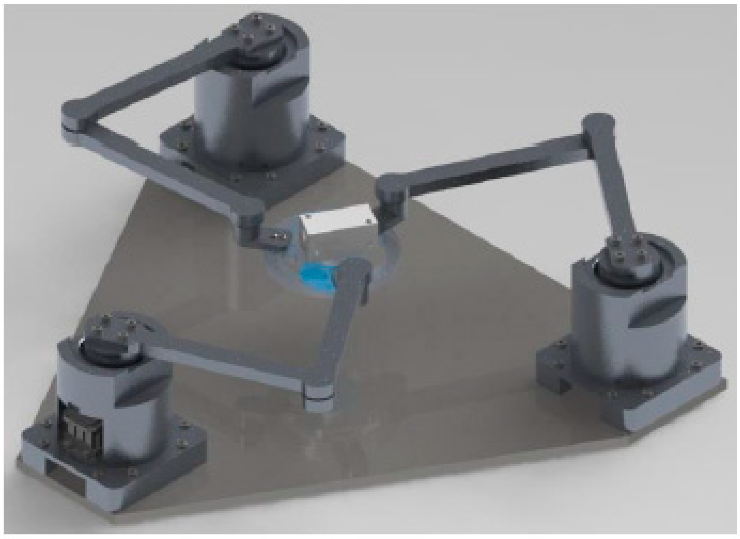
This section presents the kinematic analysis of the 3-RRR manipulator, aiming to determine the positions of the links and the end effector. Initially, a direct kinematics analysis was conducted, followed by validation through inverse kinematics analysis. The kinematic model seeks to elucidate the motion of the links within the robotic structure; through kinematic analysis, it gains significance by facilitating a comprehensive study of individual movements at each joint and their integration within the system [35].
In the field of robotics, the kinematics of a manipulator can be described by two distinct formulations: direct kinematics and inverse kinematics. The concept of kinematics pertains to the operation that determines the position and orientation of the end effector of the chain comprising the device. Conversely, inverse kinematics employs methods to ascertain the values of the generalized coordinates necessary for a kinematic chain to reach a specified position and orientation [36]. In this study, mathematical models will be formulated to conduct direct and inverse kinematic analyses of the 3-RRR parallel manipulator. Figure 1 depicts the 3RRR planar parallel manipulator designed in 3D using the SOLIDWORKS program.
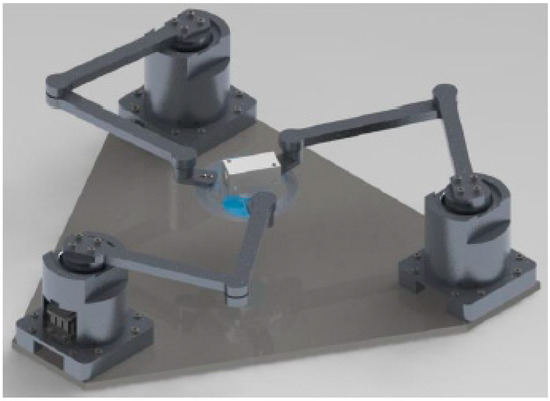
Figure 1.
3-RRR Manipulator.
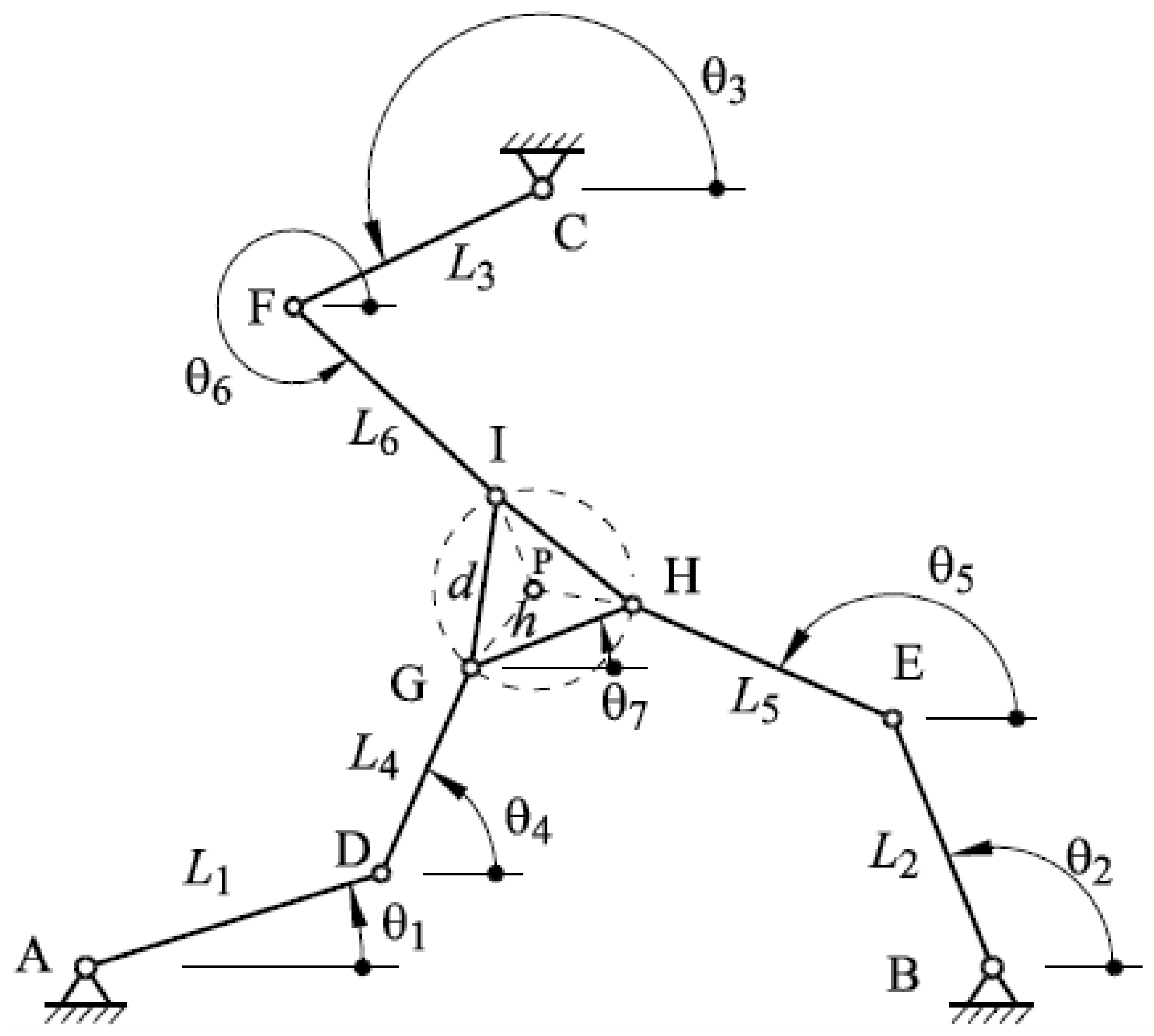
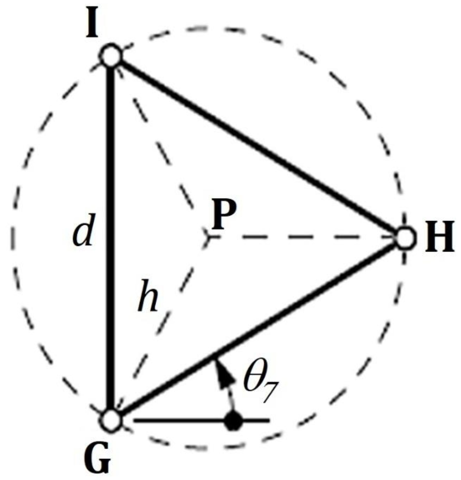
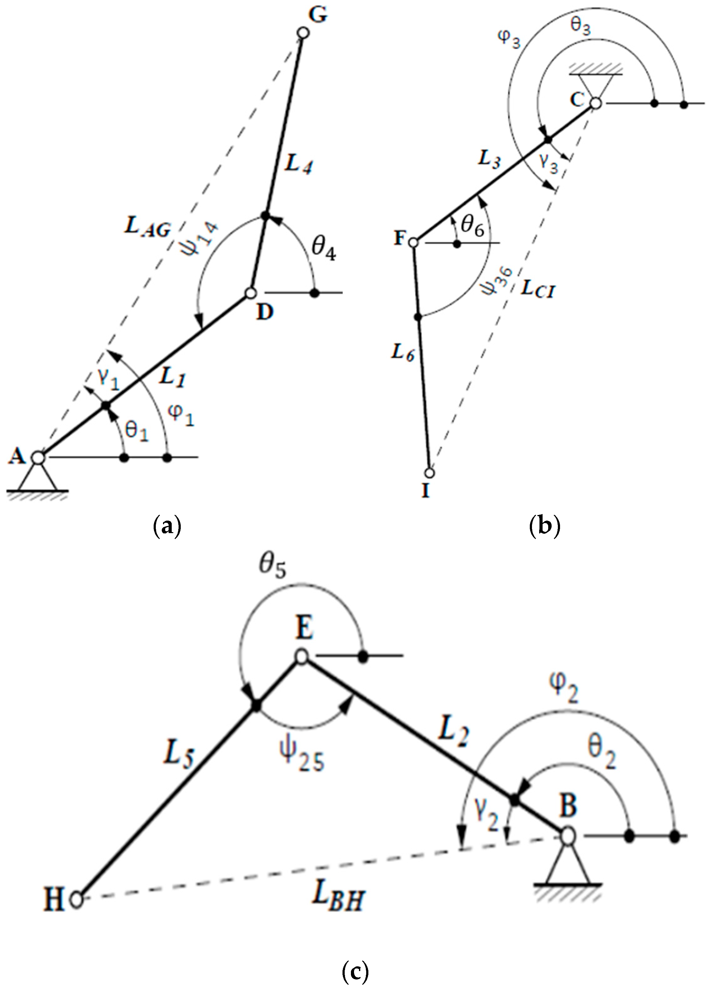
The direct kinematics analysis is based on Figure 2. This analysis requires determining the angular coordinates of the actuators, , , knowing the position and orientation of the terminal element. The 3-RRR planar parallel mechanism is now decomposed into three chains, to determine the geometric linking equations.
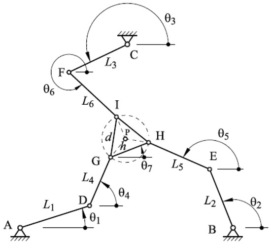
Figure 2.
Description of the geometric variables of the 3-RRR manipulator.
Knowing the position of the terminal element () and the orientation of the terminal element, the orientations of the links , , , , , and are obtained from the system of Equations (1)–(6), using the Newton–Raphson method.
When performing the path and vector calculations using points A, B, and C as references, the following loop equations are obtained. The loop vector analysis for is as follows:
Route and vector calculation are established to analyze the loop . Next, the following kinematic equations are obtained.
Finally, the route and vector calculation for the chain, , will be carried out.
2.2. Inverse Kinematics
This section presents the development of inverse kinematics for the 3-RRR closed kinematic chain parallel manipulator. The first phase starts with the mobile platform, as shown in Figure 3.
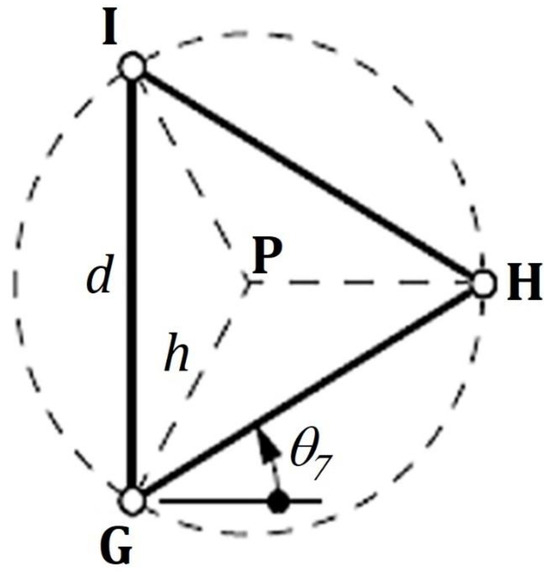
Figure 3.
Mobile Platform.
Kinematic equations of the mobile platform:
Then, in the next phase, the three links where the inverse kinematics is applied are shown (Figure 4).
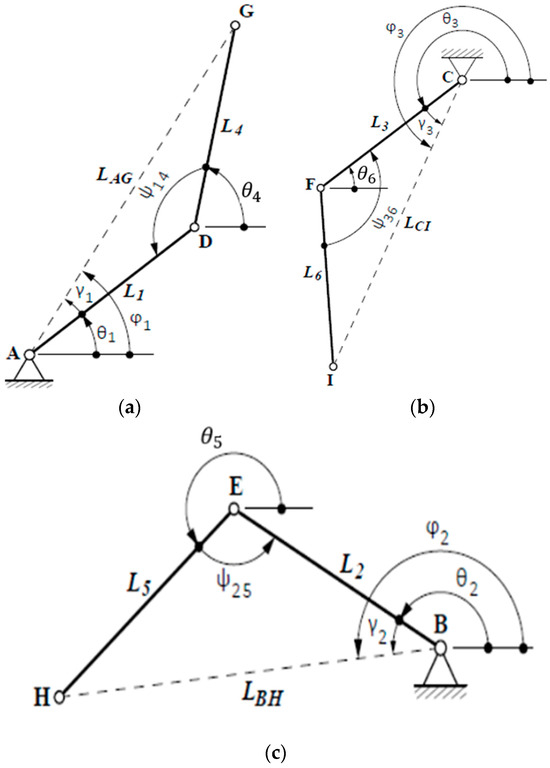
Figure 4.
Uncoupled kinematic chains for analysis. (a) Chain ; (b) Chain ; and (c) Chain .
The inverse kinematics equations for each of the uncoupled links are shown below.
For the link , the following equations are obtained:
For the chain , the following equations are obtained:
Finally, for the chain (), the following equations are obtained:
The aforementioned shows and visualizes the calculation and development of the kinematic chains of the manipulator in relation to the formulation of the direct and inverse kinematics of the 3-RRR planar parallel manipulator.
2.3. Manipulator Dynamics
This section shows the development and calculation to determine the motor torque required in the actuators. The energy method was applied as shown in Equation (28).
When observing the equation, the motor torque is the torque required by each servomotor, indicates the angular speed of the link, and the operator (∙) indicates the internal product between the two vectors and , which represent the force and speed in the terminal element.
For the analysis of kinetic energy, it is determined by Equation (29).
The variable k represents the kinetic energy of the mechanism, is the energy of the moving platform, and () is the sum of the energy of the cranks and couplers.
Finally, the motor torques of each of the actuators 1, 2, and 3 of the manipulator are obtained, as observed in the following equations.
The equations presented above use the energy method and kinetic energy to determine the torque.
2.4. Camera Calibration
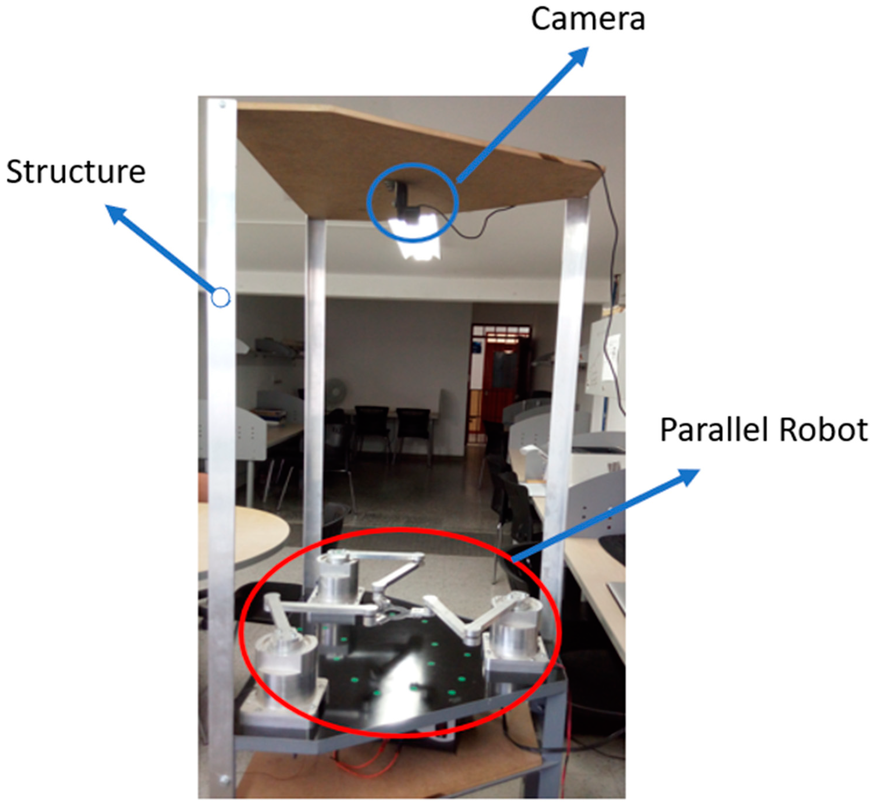
In this section, the calibration procedure for the Logitech C920 camera (manufactured in Logitech, Taipei, Taiwan) with a resolution of 1980 × 1080 pixels is described. The visual sensor used for object determination was attached to the upper part of the manipulator, with a rigid structure adapted to hold the camera, as shown in Figure 5.

Figure 5.
Support structure for the camera.
Figure 6 shows the chessboard used for calibration, with each square measuring 22 mm by 22 mm. The calibration process was carried out using the Mathworks MATLAB 2021® software, which processes the pattern image to determine a reference point, indicated by the yellow box (checkboard origin). The green circles (detected points, totaling 24) represent the points detected in the calibration pattern; these points are essential for making an estimate using the Zhang et al. model [19].
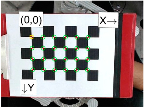
Figure 6.
Calibration pattern. The yellow box indicates the origin within the chess pattern. The red crosses represent the vertices, and the green circle indicates the centers.
Additionally, there are red rear projection points (reprojected points), indicating the alignment of the detected point with the rear projected point. The quality of the calibration is determined by this alignment, as rear projection depends on the elimination of projective distortion. For a correct estimate, 10 to 20 photos should be captured at appropriate positions and distances from the camera, ensuring that the pattern is not parallel to the camera plane. For this project, 20 captures were taken to calibrate the camera.
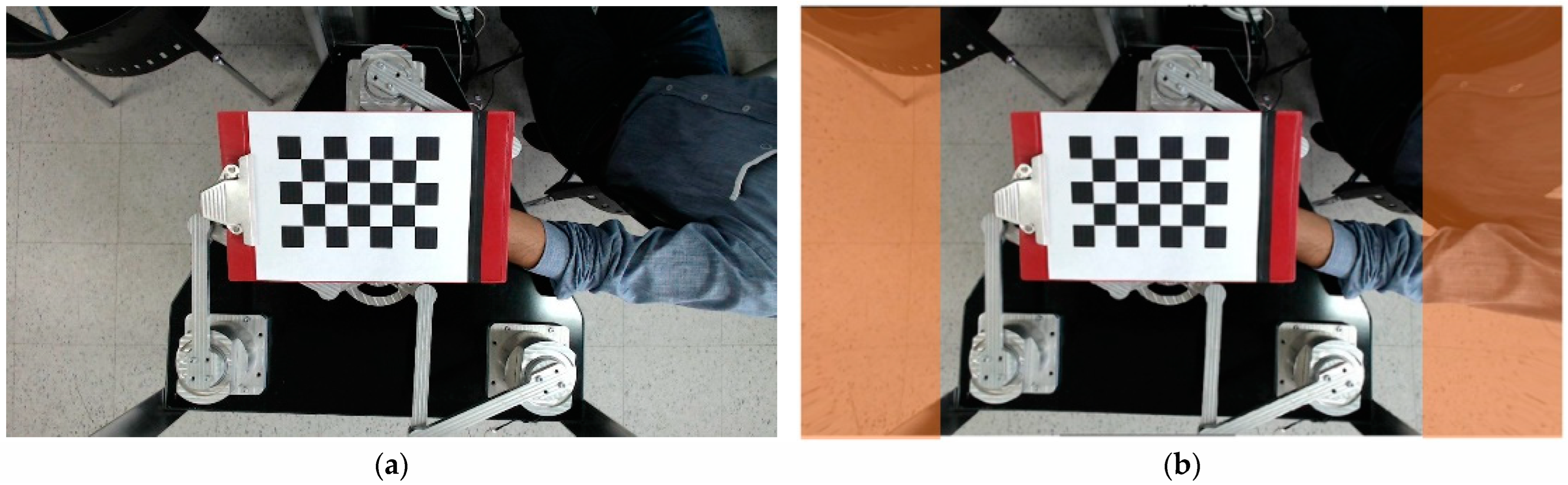
Once calibration is established, an image without projective distortion is obtained, as evidenced by comparing Figure 7a,b, where the orange area shows the correction applied to the image, establishing a rearrangement of the pixels when the calibration process is applied.

Figure 7.
(a) Image without projective distortion. (b) Image correction after calibration.
This calibration was achieved using the MATLAB® application interface. After calibrating, the camera parameters, such as intrinsic and extrinsic parameters, were saved. The calibration parameters were then applied to the image to create a distortion-free image using the “undistortImage” function in MATLAB®. The corrected image was then used to process vision algorithms for object detection.
2.5. Vision System
This section describes the application of an algorithm developed in MATLAB® for detecting color and semantic characteristics within objects. One of the most commonly used algorithms for object detection is based on color. The color detection process begins with the decomposition of the image into RGB layers. Each layer that constitutes the image is defined by a two-dimensional function, , where () are the coordinates of each pixel.
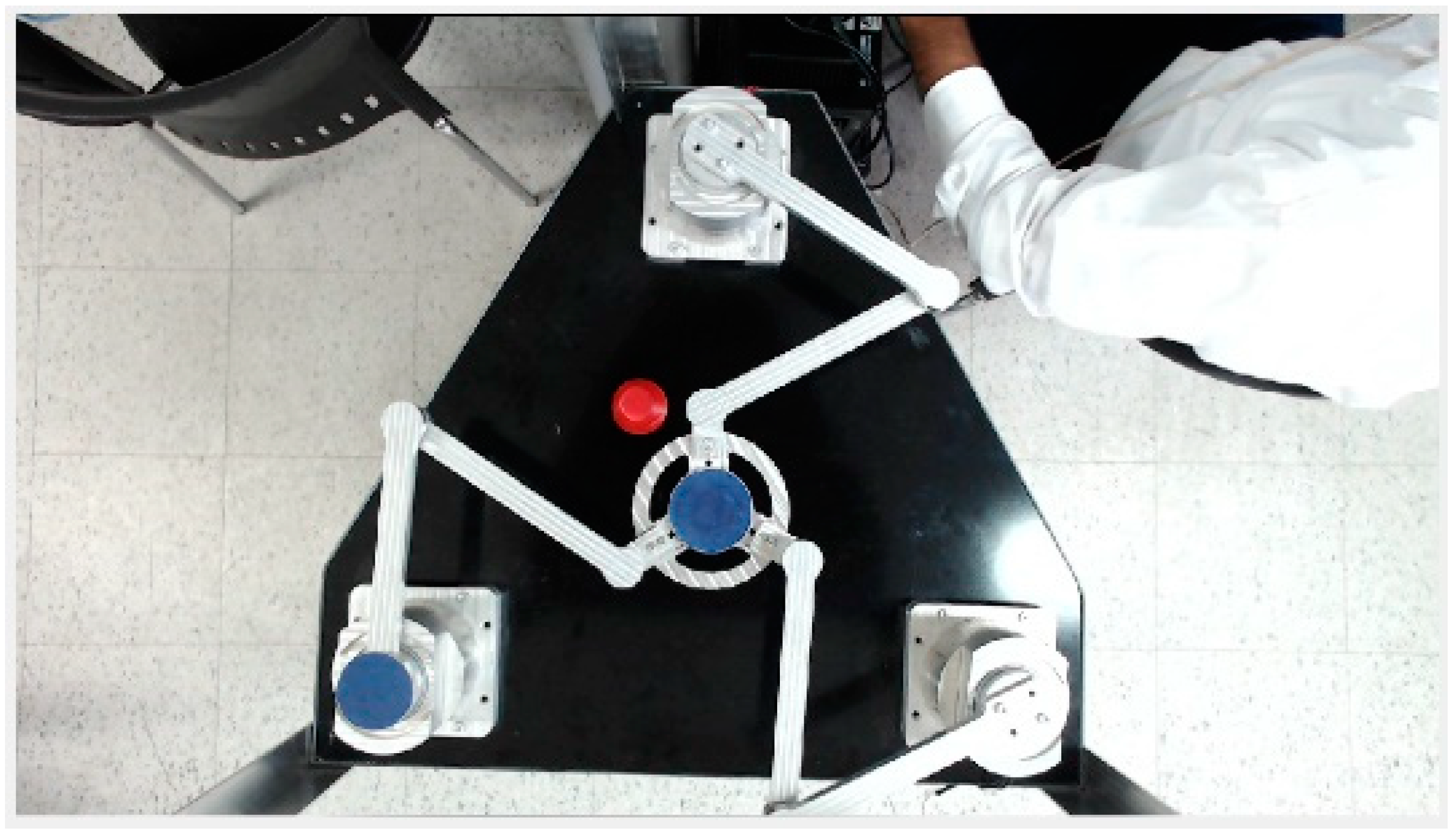
Figure 8 shows the capture of the manipulator from the top, where there are two blue sections. Firstly, the detection of the blue and red color of the image is established from the segmentation.

Figure 8.
Image capture of the parallel manipulator.
To proceed with color extraction, the image must be decomposed into several layers. When capturing each image, it must be decomposed into its RGB layers. The mathematical formulation for calculating the back projection error was not included, as the MATLAB 2021® Camera Calibration Toolbox (sourced from MathWorks, located in Natick, MA, USA) handles this calculation automatically. This toolbox provides an easy-to-use interface for estimating camera parameters, including back projection error, without the need for custom source code. Using the MATLAB® Image Processing Toolbox, the red layer is extracted from the image, which has been resized to 640 × 480 pixels. This resolution was chosen to reduce the computational load required for processing the pixels in the images. Under this resolution, both the red and blue layers are extracted. Initially, the image is converted to HSV color space using the MATLAB® function “rgb2hsv”. For red color detection, a threshold range of 0 to 0.1 is applied. For blue color detection, thresholds between 0.55 and 0.75 are used. Finally, a saturation threshold of 0.4 and a value threshold of 0.2 are applied to enhance the detection results. Once the adjusted values are in place, the binary masks for the red and blue colors are developed and then applied to the original images with the MATLAB® function “bsxfun”. As a result, Figure 9 and Figure 10 are obtained.
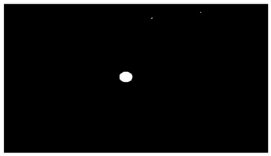
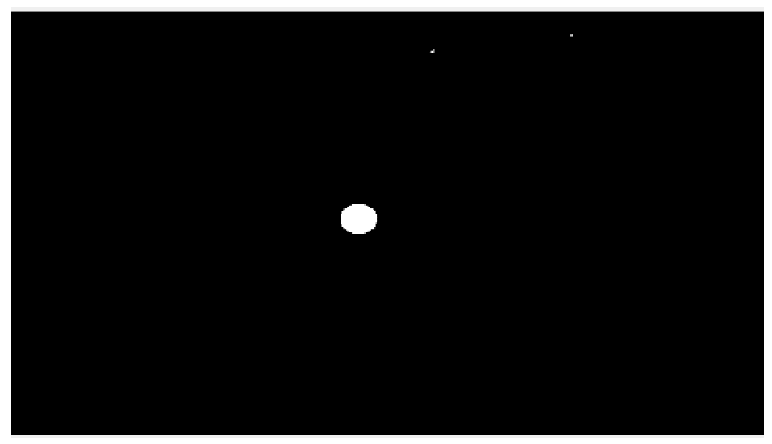
Figure 9.
Binary image of the red layer.

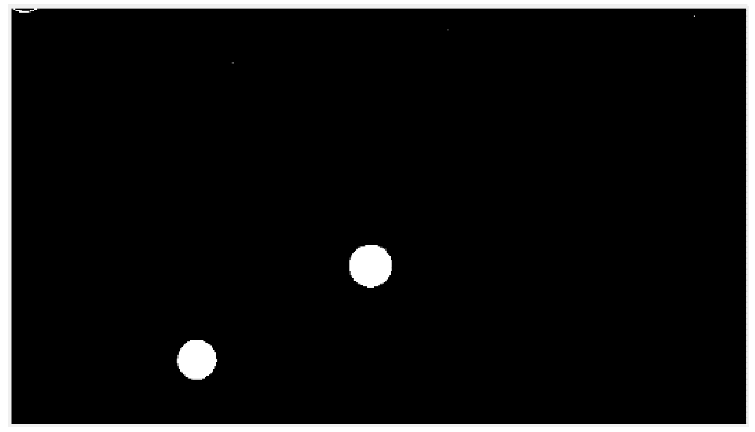
Figure 10.
Binary image of the blue layer.
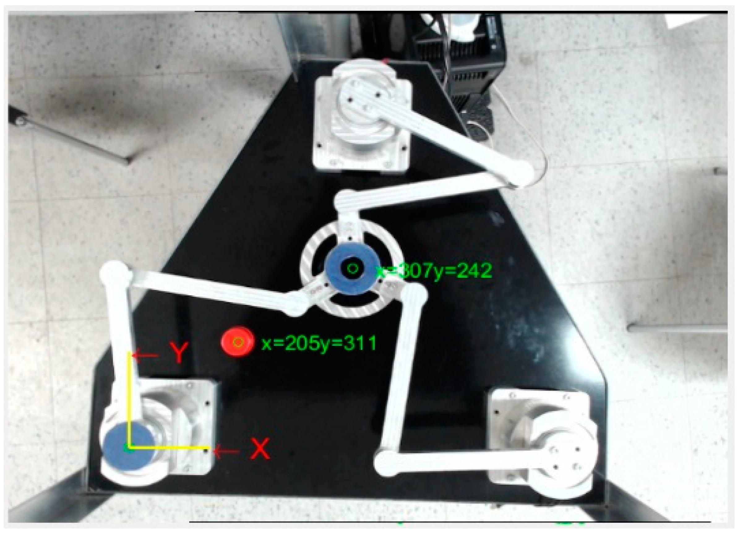
Once the colors in the images are segmented, the centroids of the detected elements are calculated. This is carried out using the “regionprops” function in MATLAB®, which provides the centroid coordinates for each detected object. The result of this calculation is shown in Figure 11.
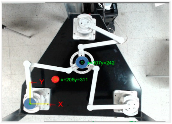
Figure 11.
Detection of the object, final actuator, and reference frame of the manipulator.
After determining the detection of the object, the origin, and the end effector, the homography process for image stabilization is developed.
2.6. Descriptors
In this section, a series of markers were positioned within the manipulator’s workspace, totaling 20 elements, aiming to establish correspondences and compute a homography for video stabilization. The application of the SURF algorithm is demonstrated below, where 40 characteristic points are identified across two images, as depicted in Figure 12a,b.
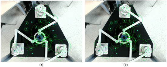
Figure 12.
(a) Application of the SURF algorithm—Image 1. (b) Application of the SURF algorithm—Image 2.
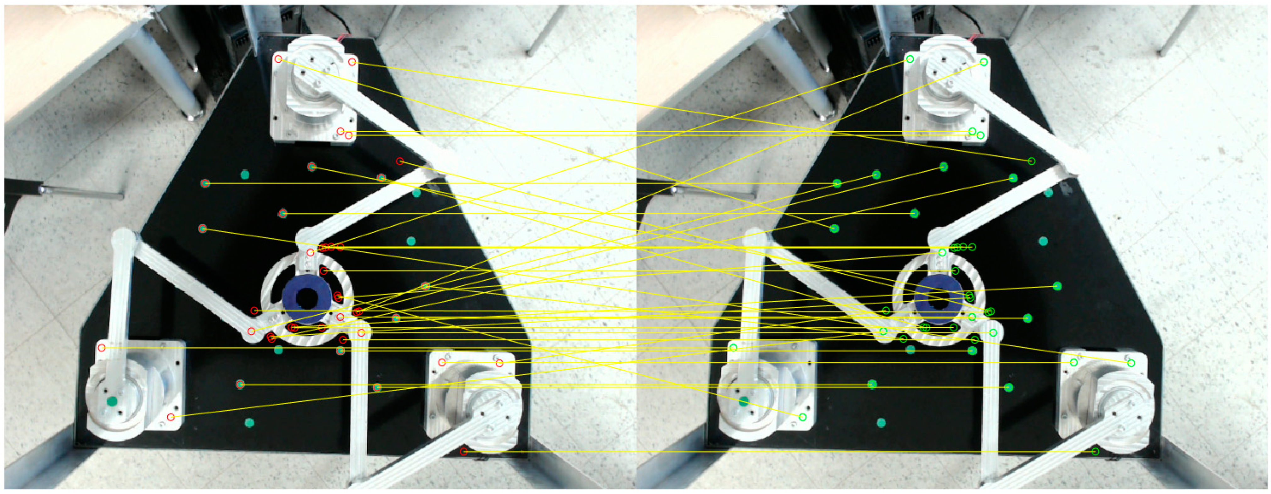
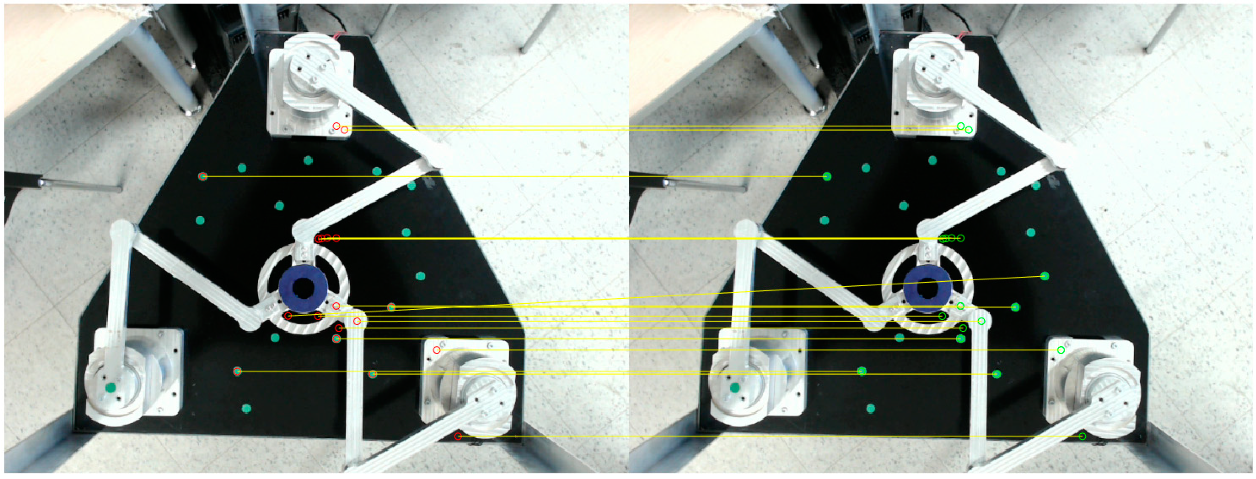
Upon establishing characteristic points in both images, putative correspondences are determined, as depicted in Figure 13.
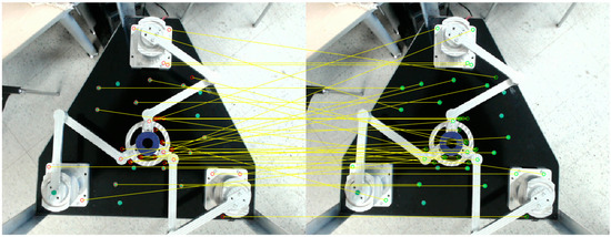
Figure 13.
Putative correspondences between image 1 and image 2. The red circular indicators are parts that are taken from the left image as characteristics and are linked to the characteristics and indicators of the right image, which are then connected by means of the yellow line.
When determining correspondences, it is noted that some do not coincide. To address this issue, it is imperative to establish a method enabling the calculation of appropriate correspondences in both images. This method, known as RANSAC, serves this purpose.
RANSAC is an iterative method facilitating the calculation of parameters for a mathematical model based on a set of observed data, which may include outliers—data points significantly distant from the others. These outliers are identified and addressed within the algorithm. Though generally non-deterministic, RANSAC yields robust results contingent upon the number of iterations assigned to it [37].
In our study, RANSAC was utilized to estimate homography from corresponding points obtained through the SURF descriptor. The aim was to determine the minimal number of points necessary for estimating the model and assess the conformity of these data with the estimated model. This procedure was implemented using the MATLAB® program, as depicted in Figure 14.
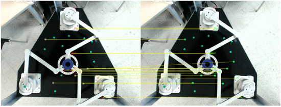
Figure 14.
Putative correspondences. The red sections (Left Image) and the green sections (Right Image) indicate the putative correspondences between both images, which are linked by a yellow line.
The method was executed and refined through 5000 iterations, employing an estimation threshold of 0.0001, which specifies the distance for identifying outliers. In total, 18 putative correspondences were derived from 40 characteristic data points extracted from both images using the SURF descriptor.
2.7. Homography
In this section, homography calculation commenced by initially detecting green markers within the working section of the manipulator. Each marker corresponds to the manipulator’s reference frame, with their respective positions calculated relative to a CAD model, as illustrated in Figure 15. These marker positions were measured in centimeters, totaling 19 markers. The process was executed using SOLIDWORKS 2020.
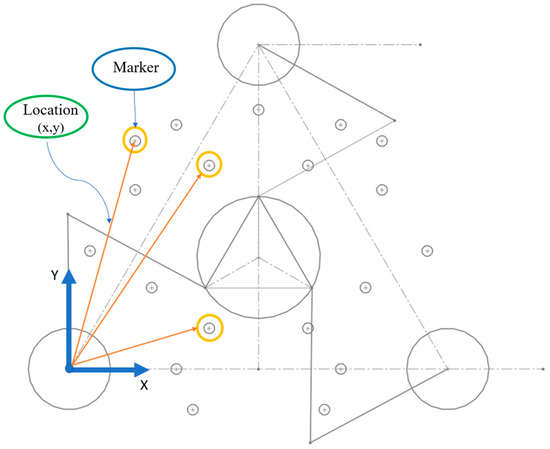
Figure 15.
Location of markers in the work area.
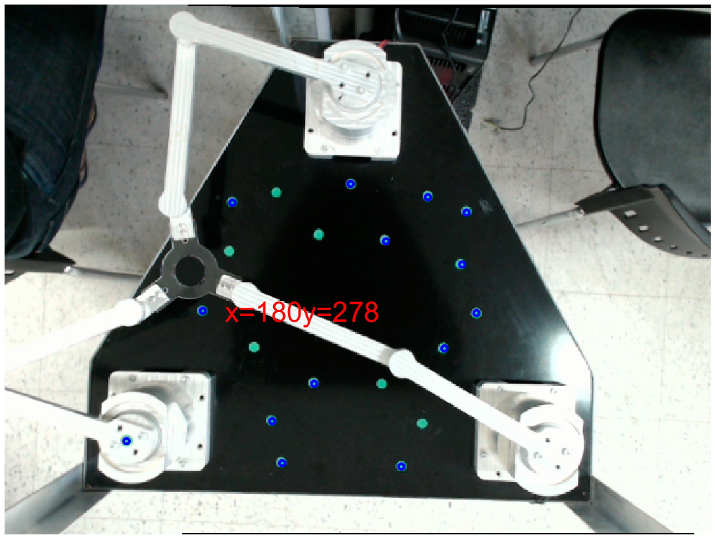
To determine the homography matrix for video stabilization, the first phase involves calculating fixed points (drawn in CAD and estimated under the reference frame) and displaced points (points located on the manipulator’s work plane). For the fixed point stage, a random number of points were created in the work area, drawn and created in CAD using the SOLIDWORKS program. Each point was extracted with a total of 19 markers, and their positions () were calculated. Similarly, other points were estimated and located in the work area of the manipulator, determined as displaced points measured under the origin of the manipulator, as shown in Figure 16. The next step was to detect these points and apply the MATLAB® “fitgeotrans” function to determine the homography matrix H. After matrix H is calculated, it is applied to the image using the “imwarp” function to transform the image for further analysis. It is important to note that the object is not evident in the image during this process, as only the transformation matrix H is being determined. Therefore, the area must be cleared of all objects.
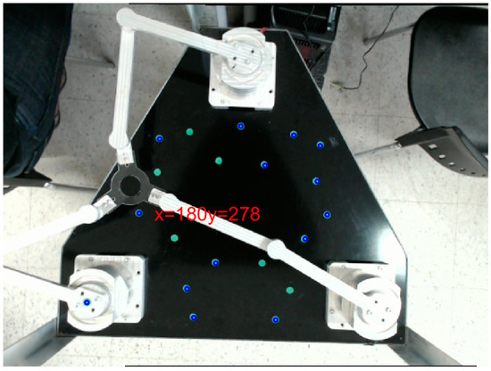
Figure 16.
Detection of markers to determine their centroids. The blue circular sections show the centroids of each green circular element located within the manipulator’s work area, indicating the coordinates of each element.
The homography process aimed at achieving image stabilization, as the structure housing the visual sensor lacked sufficient rigidity and could potentially introduce errors in object localization. The steps to determine homography are as follows:
- Define the correspondence points from both the fixed image (CAD) and the estimated points (located manually in the work area of the planar manipulator).
- Locate the fixed and estimated position data in vectors.
- Once the coordinates of the correspondences are determined, calculate the homography matrix “H” using the MATLAB® “fitgeotrans” function, which depends on the vectors.
- Apply the calculated matrix “H” to the image to be transformed using the MATLAB® “imwarp” function.
- After transforming the image, proceed with the detection of red (object) and blue (origin) objects and their centroids from the transformed image using the H matrix.
The homography process was carried out to establish image stabilization, as the structure holding the visual sensor was not rigid enough, potentially generating errors in the location of the object.
2.8. Control System
In this section, an open-loop kinematic control system is implemented, as illustrated in Figure 17. This system takes an image captured by the camera as input. The captured image is then processed by a computer vision algorithm to extract the features of the target object. These extracted coordinates are subsequently forwarded to the inverse kinematics module. In cases where the object becomes occluded, the Kalman algorithm predicts the next position by leveraging previous object data, which are then relayed to the inverse kinematics module.
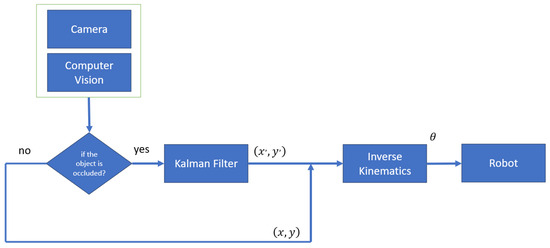
Figure 17.
Open-loop kinematic control.
2.9. Visual Servo Control
The visual servo control technique is applied in robotics to use visual information for controlling the robot’s movement. This process integrates image processing and system control, enabling the robot to accurately and autonomously perform tasks using visual feedback. Two primary configurations of visual servo control techniques are Eye-in-Hand and Eye-to-Hand. In the Eye-in-Hand configuration, the camera is mounted directly on the robot’s end effector. The vision system moves with the robot, providing a dynamic view of the environment from the perspective of the end effector. In contrast, the Eye-to-Hand configuration places the camera in an external position to observe the work area, offering a static panorama of the environment that includes both the robot and the object of interest. Visual servo control techniques can be described by two mathematical models: Image-Based Visual Servoing (IBVS) and Position-Based Visual Servoing (PBVS). The IBVS model relies directly on the coordinates of the points of interest in the image, while the PBVS model uses the estimated position and orientation of the object in 3D space. Given the robot’s morphology, the best configuration for the manipulator was determined to be the Eye-to-Hand visual servo control technique using the PBVS mathematical model.
In this section, Eye-to-Hand configuration was implemented due to the inability to establish the first configuration, attributed to the manipulator’s morphology and the considerable disparity in camera placement. This complexity arises from the limited workspace, making camera attachment challenging. The configuration applied to the closed kinematic chain parallel manipulator is shown in Figure 18.
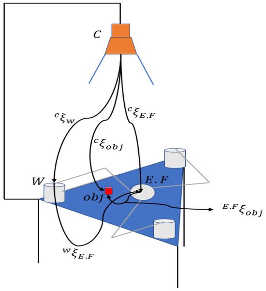
Figure 18.
Eye-to-hand configuration applied to the 3-RRR parallel manipulator.
In this configuration, the operator represents the homogeneous transformation matrix that relates the coordinates of points in 3D space with their coordinates in the image.
The parameter represents the camera, defines the origin of the robot, defines the object, and defines the end effector. The matrix is shown in Equation (33).
The homogeneous transformation matrix consists of a rotation matrix , a translation vector , a scale vector made up of zeros, and a value of 1 in the () position representing the perspective. This matrix describes the robot’s pose and transforms coordinates from the robot’s coordinate system to the camera’s coordinate system and vice versa. To determine the orientation and pose of the target and the end effector, Equation (34) is used:
This mathematical equation calculates the orientation between the object, the camera, and the manipulator concerning the manipulator’s coordinate system. This entire process was implemented in MATLAB 2021®.
2.10. Kalman Filter
This section outlines the Kalman filter’s implementation based on previous studies [38,39,40] to estimate real-time object position and motion. In this study, the Kalman filter is employed to enhance the accuracy of position estimation for a moving object, particularly during occlusions. The initial position data (x, y) are obtained from the vision algorithm when the object is first detected by the camera. To estimate the initial velocity, the difference between successive position data points is calculated, assuming a time interval (∆t) of 1 s. The objective is to enable the parallel manipulator, characterized by a closed kinematic chain and a 3-RRR configuration, to follow the trajectory of the target via its end effector.
The methodology for detection, data acquisition, and processing for position estimation is described in the following items.
- Capture and acquisition of semantic features for the target:
- Sequential capture of the target using the visual sensor.
- Calculation of the target’s semantic characteristics through computer vision techniques [40,41].
- Kalman filter initialization:
- Establishing the object model, incorporating position and velocity.
- Initialization of the state error covariance and measurement error covariance matrices with estimated values.
- Implementation of the state transition and observation matrices based on the object model.
- State prediction:
- The Kalman filter predicts the object’s current state for each iteration, using the state model and previous measurements.
- Predictions are based on the previous step’s estimation state and the object motion model.
- Measurement update:
- 2D coordinates obtained from the computer vision system are used as measurements to refine the object’s estimate.
- The Kalman filter [42] merges the state prediction with new measurements, weighting each according to their reliability, determined by the covariance matrices.
- Optimal estimation status:
- Following the measurement update, the Kalman filter yields the optimal current state estimate of the object, including position and velocity [42].
- This estimation controls the manipulator’s motion for effective object tracking.
- Iteration and update:
- This process repeats for each new frame captured by the computer vision system, continuously refining the object’s state estimate for precise and smooth real-time tracking [38,43].
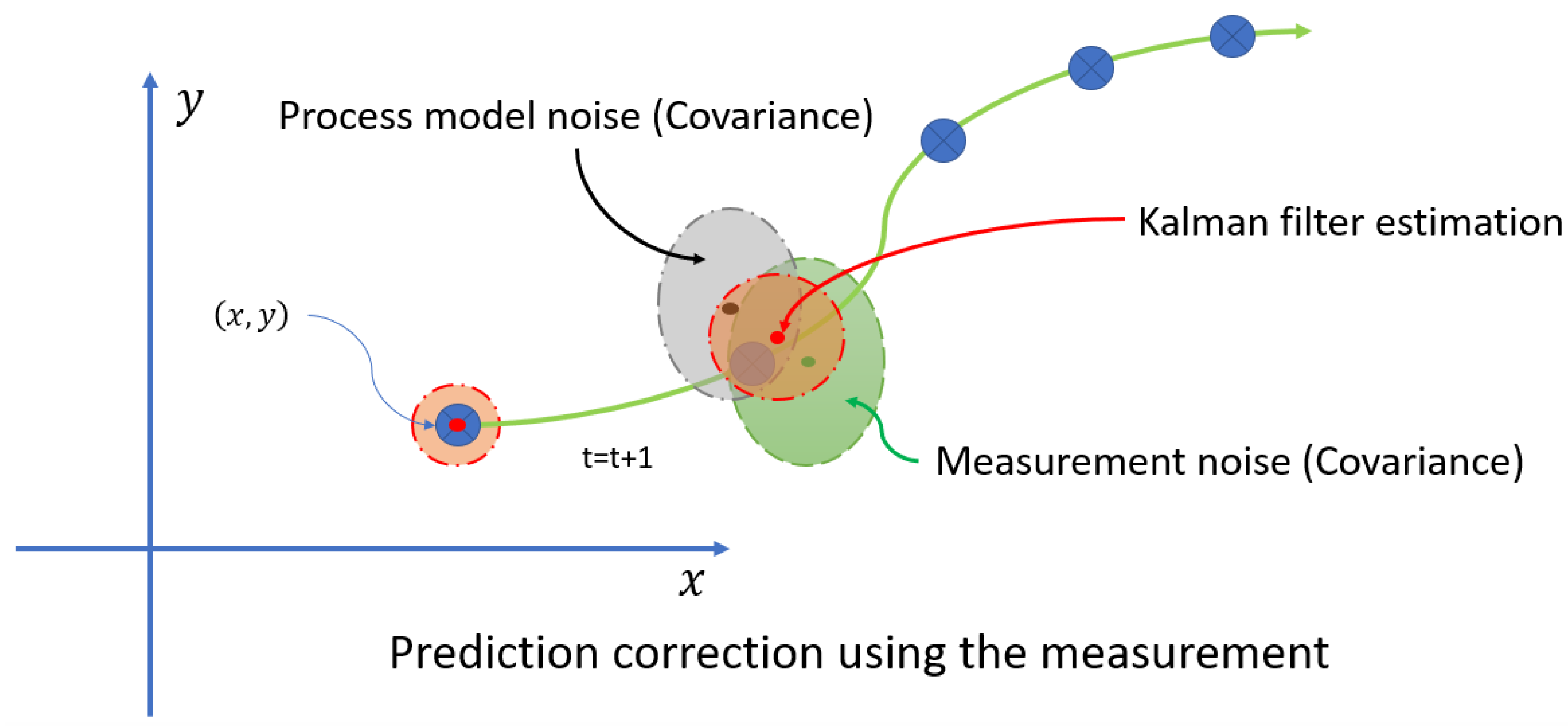
The main challenge encountered was the occlusion of the moving object caused by the base located on the end effector. Each time the end effector moved, it occluded the object. To address this issue, the Kalman filter was proposed as a solution due to its computational efficiency. The Kalman filter is ideal for this project because it enables real-time processing with a low computational load, which is crucial for vision and prediction systems. This filter not only estimates the current state but also predicts future states, an essential capability when objects are occluded or temporarily out of the field of view. Additionally, the Kalman filter effectively handles measurement uncertainties and noise by combining noisy measurements with prior knowledge of the system, resulting in more accurate and reliable estimates, as demonstrated in Figure 19 and Figure 20.
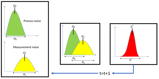
Figure 19.
Estimation process.
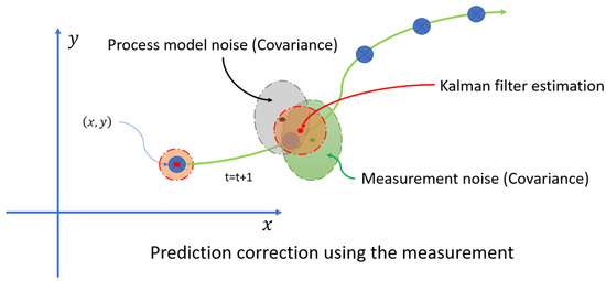
Figure 20.
Prediction process using measurement noise and process noise.
It is also a general problem of the paper that the procedures used in various steps of the algorithm are inadequately described, which does not allow them to be replicated. Moreover, the authors in most cases do not discuss how they deal with errors and noise.
Although other estimation methodologies were considered, such as particle filters, extended Kalman filters, neural networks, and machine learning methods, these options were ultimately discarded. These alternatives require significant data storage and high computational capacity, which was not feasible for this project. The process carried out to estimate the future position is detailed below.
2.10.1. System Modeling
In the first phase, the position and speed of the object in constant motion in 2D space are modeled. The vector is created, as seen in Equation (35):
The equation of the state of the discrete system is described as presented in Equation (36).
where the parameter F is called the transition matrix. The matrix F is shown in Equation (37), with a Δt = 1 s:
The term is defined as the noise of the process, which is established as a vector with a normal distribution with zero mean and covariance Q. The matrix F describes the next state of the system. That is, it estimates the next state of the system based on the current state.
The measurement model, , for the positions is defined in Equation (38):
where the parameter is the measurement noise, which is a normally distributed random vector with zero mean and covariance R. The observation matrix H is defined as:
The observation matrix H describes the relationship between the state of the system and the observed measurements.
2.10.2. Estimation of Q and R Parameters
The Q matrix describes the uncertainty in the process model. A heuristic approach was used to analyze the Q matrix based on the expected variability of the process. This approach utilized historical data of the true state () and the estimated state (), where position and speed data are presented in a vector. The differences were calculated using the following Equations (40) and (41):
To determine the R matrix, the covariance of the uncertainties in the measurements of the visual sensor or camera was calculated. To estimate the parameter R, data were taken from the positions established by the visual sensor M, and then its covariance was calculated. The process is shown below from Equations (42) and (43).
The methodology to calculate the R and Q matrices is based on system measurements and results. In this case, the R and Q values can also be determined empirically. Two constant parameters, r and q, can be estimated to define these values. The parameter q represents the magnitude of the process noise, while r defines the measurement noise. These constants can be estimated empirically based on the system’s characteristics and performance. If the estimates are too noisy, the parameter q should be decreased. Conversely, if the response is too slow, q should be increased. For the parameter r, if the Kalman filter’s measurements are ignored, r should be decreased. However, if the measurements dominate the process, significantly influencing the estimate, r should be increased.
The process noise covariance matrix Q is estimated using a few movement trajectories, comparing the theoretical position and torque model with actual measured data. Although the current estimation shows some discrepancies due to limited samples, increasing the number of trajectories could improve the accuracy of the Q matrix. The measurement noise covariance matrix R is based on the position data provided by the camera. Measurement errors are calculated by comparing the true positions (from a noise-free trajectory simulation) with the measured positions, providing a basis for the R matrix. These calibrated matrices enable the Kalman filter to optimally estimate the position of the object, even when measurements are unavailable due to occlusion, thereby ensuring continuous and accurate tracking.
2.10.3. Initialization of the Kalman Filter
To perform the initialization of the estimated initial state , for the covariance of the initial state , the noise matrices Q and R are also defined. The initialization process of the matrices F and H was programmed in MATLAB 2021® as follows.
To perform the initialization of the initial state , for the covariance of the initial state P, where the variance of the initial estimates of position and and velocity and , with initial uncertainties which are estimated from historical data, are taken, the noise matrices and are also defined. The initialization process of the F and H matrices was programmed in MATLAB® as follows.
Initial parameters for the Kalman filter:
The matrix P is the initial covariance matrix which initializes the variances of the position and velocity.
2.10.4. Kalman Filter Algorithm
The Kalman filter operates in two main stages: the prediction stage and update stage. The detailed steps are as follows:
Apriori state prediction:
State error covariance prediction:
Update stage
Kalman gain:
Update the estimated status with the new measurement:
State error covariance update:
This algorithm allows for the determination and estimation of the object’s position, even in the absence of measurements or in the presence of noise. In Equation (47), the estimated state data under system and measurement noise conditions result in the new positions (), which are then calculated and fed back to the manipulator for tracking and detecting the object. It should be noted that there were no known inputs in the system since only kinematic control was established.
3. Results and Analysis
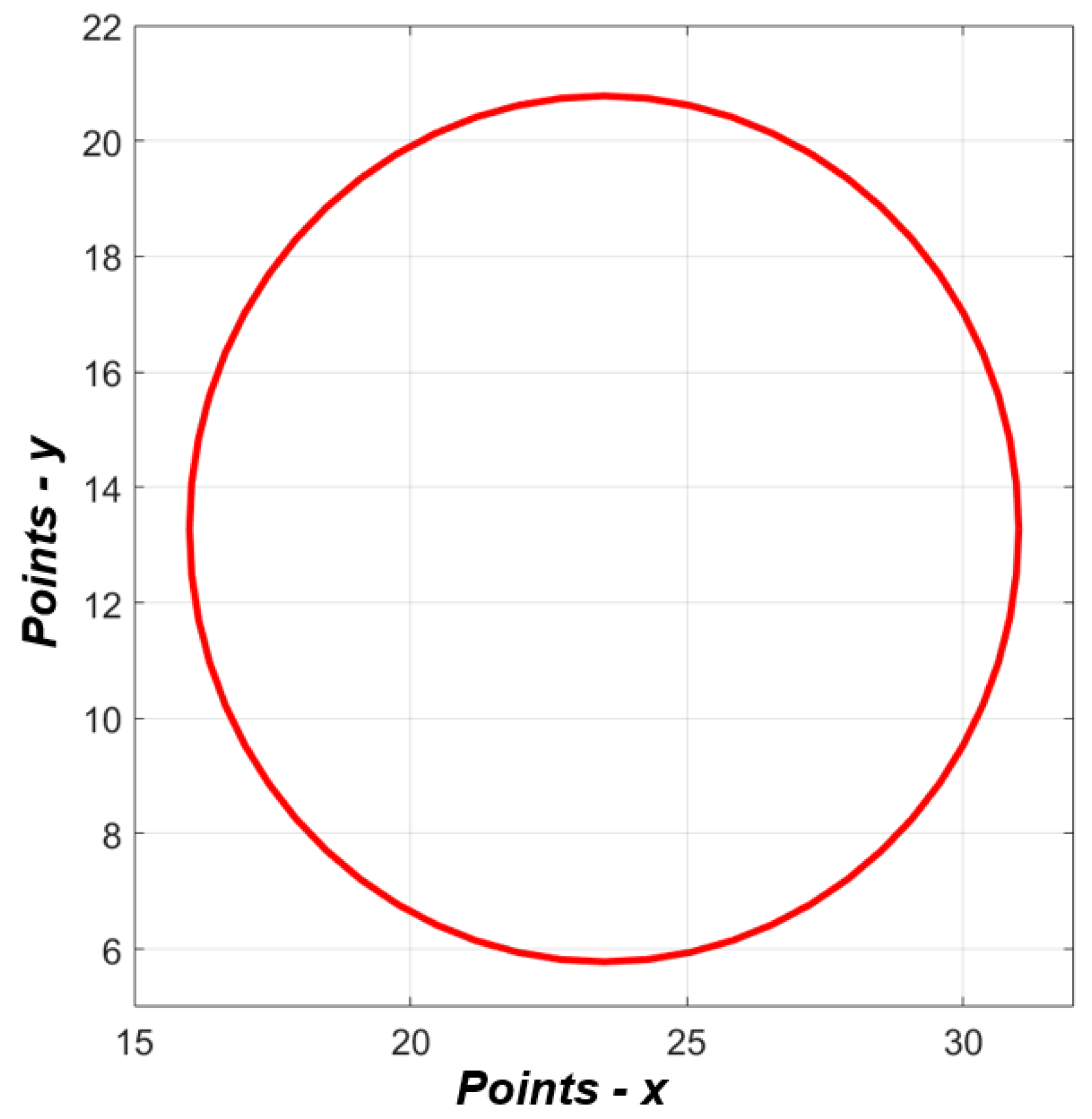
In the first instance, data were taken from a trajectory based on a circular path, as shown in Figure 21. The positions () along this circular trajectory were sent to the inverse kinematics algorithm, resulting in theoretical angular position data. These values were then compared with the processed and generated angular position data from the servomotors. In this section, both theoretical and real data are observed. The theoretical data refer to the values established and generated by the dynamic equations of the three links of the manipulator. The real data, on the other hand, are the responses provided by the servomotors in terms of angular positions. It is important to note that the vision system was not activated in this phase. This was carried out to analyze and compare the inverse kinematics values of the manipulator (angular position data) against the data delivered by the servomotors. The goal was to demonstrate the correlation of values in terms of angular positions and validate the accuracy of the responses. To obtain the results, a circular trajectory was established, as illustrated in Figure 21.

Figure 21.
Circular path.
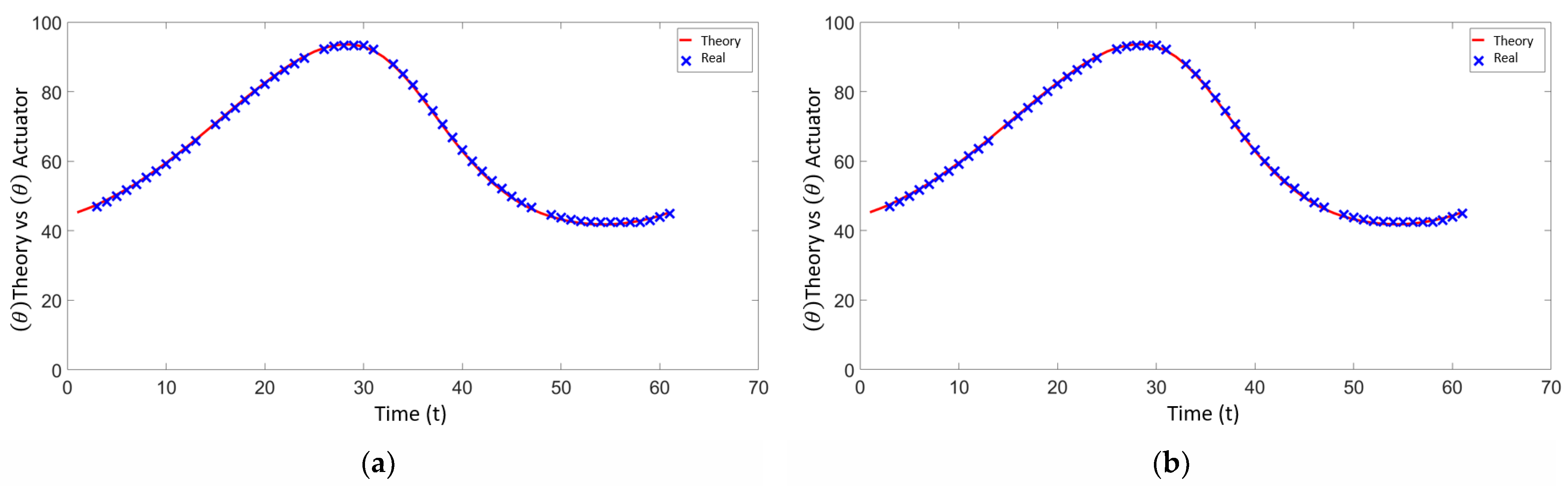
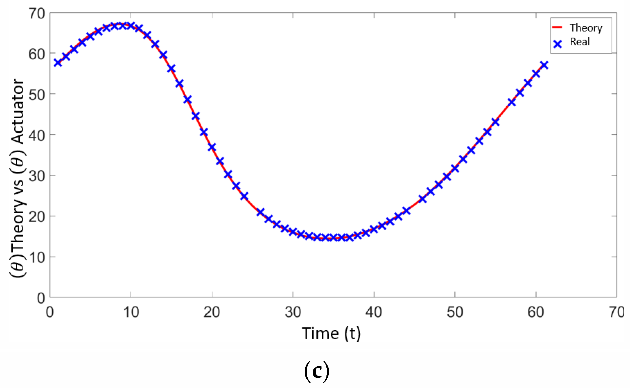
In the first phase, a circular trajectory was programmed where the positions (x, y) are sent to the inverse kinematics of the manipulator, resulting in the angular positions. This information was sent to the three servomotors for validation. Figure 22 shows the theoretical angular position data delivered by the kinematic chains, where the angles , and are analyzed with respect to the data provided by the servomotors. The red line in Figure 22 represents the theoretical angular positions provided by the inverse kinematics, while the blue line indicates the actual angular positions provided by the servomotors as feedback. This comparison helps validate the accuracy of the servomotors in following the programmed trajectory.
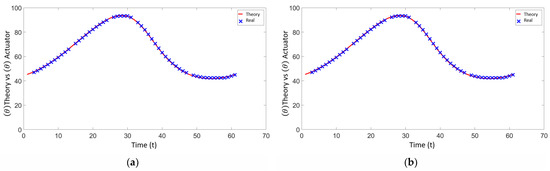
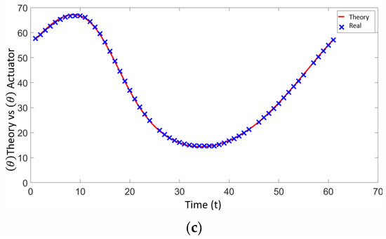
Figure 22.
(a) Angular position of servo 1—theoretical vs. real. (b) Angular position of servo 2—theoretical vs. real. (c) Angular position of servo 3—theoretical vs. real.
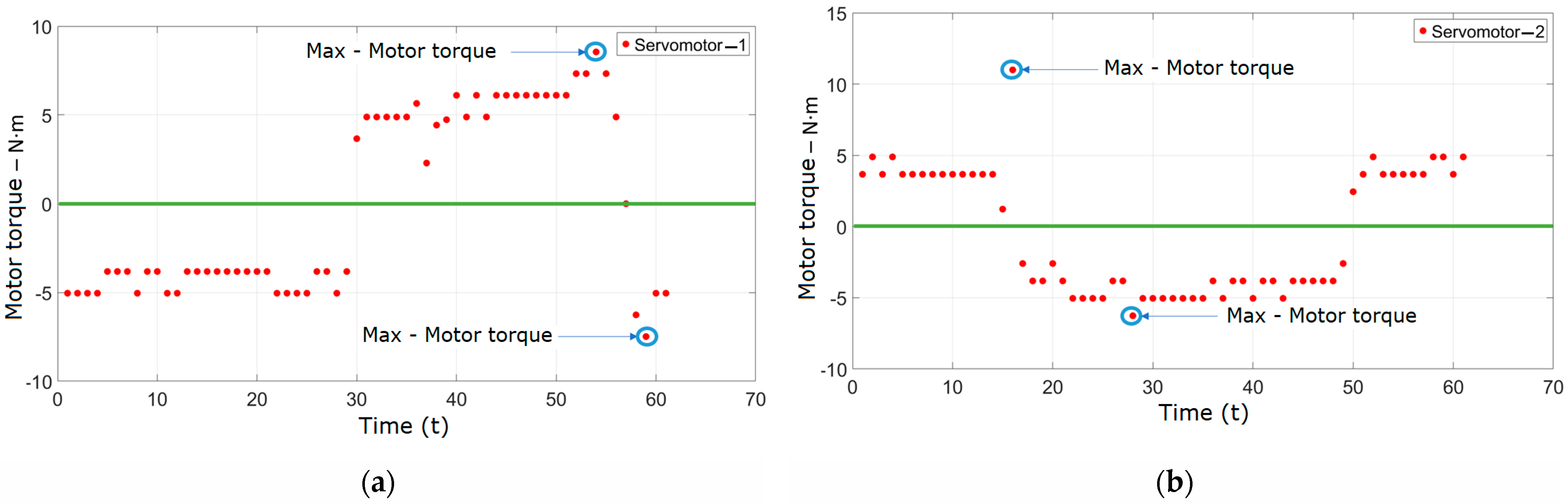
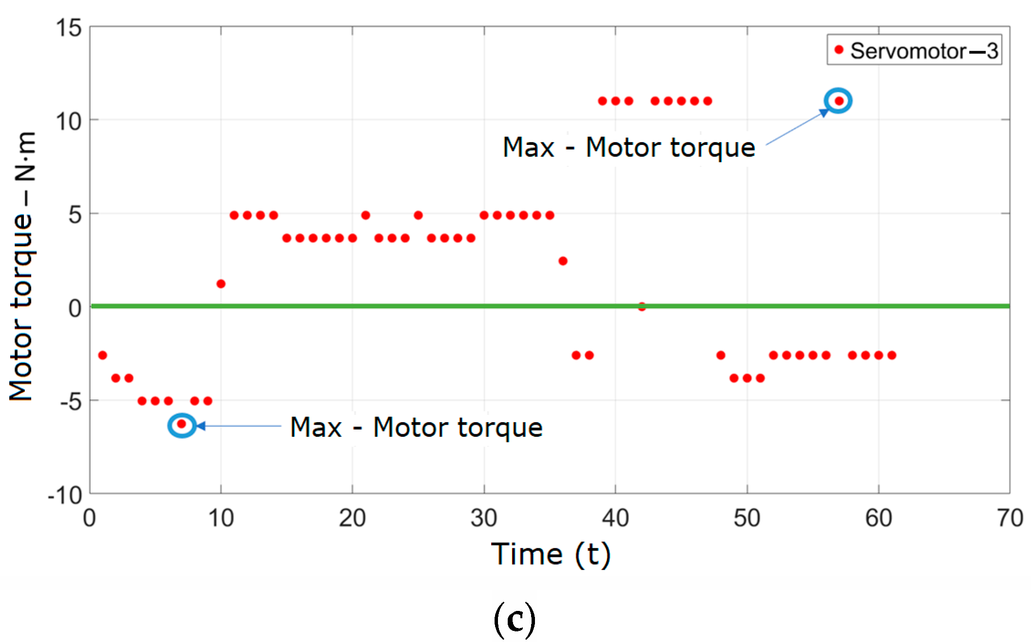
The test procedure for obtaining the data presented in Figure 23 involved running the manipulator along the predefined circular trajectory and recording the torques delivered by the servomotors at various positions along this path. These figures illustrate the real motor torques generated by each servomotor during the execution of the circular trajectory. The data help to understand the behavior and performance of the servomotors under dynamic conditions, providing insights into the torque demands and verifying the consistency of the manipulator’s response.

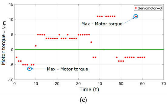
Figure 23.
(a) Motor torque—servomotor 1. (b) Motor torque—servomotor 2. (c) Motor torque—servomotor 3.
Figure 23a–c show the real data of the motor torques delivered by the MX-64T servomotors [39]. To describe the torque, a conversion from bytes to motor torque for each servomotor was established. The differentiation of movement for each motor was also determined as follows: values above zero indicate counterclockwise rotation, while values below zero indicate clockwise rotation. Each value is graphed discretely, with points representing each data shot. In these figures, the maximum torques are generated when the kinematic chain reaches its maximum extension or is close to a singularity in either the clockwise or counterclockwise direction of rotation. These torque values are provided directly by the servomotors. Figure 23a shows the data for servomotor 1 operating the kinematic chain . Figure 23b shows the torques delivered by the kinematic chain , and Figure 23c shows the torques delivered by the kinematic chain . These data are based on the programmed trajectory that was initially planned. Regarding the differences in the indicated maximum torques for servomotor 1, it is important to note that the conditions and constraints during each set of measurements can affect the maximum torque values observed.
Results of the Vision System Applying the Eye-to-Hand Visual Servo Control Configuration and the Kalman Filter
In this section, we present the results established by the aforementioned methodologies. In the first instance, as seen in the work area of the manipulator, a circular pattern is created, as shown in Figure 24. As mentioned in Section 2.8, the Eye-to-Hand configuration was established, where the camera is positioned at the top of the manipulator, providing a broader view of the work area, as seen in Figure 24. Within the same work area, a red object was established as the element to analyze, detect, and move manually. The end effector, initially transparent, was later replaced with a metal base to generate occlusions and test the established algorithms.
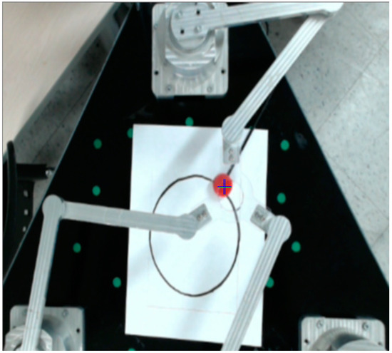
Figure 24.
Object detection.
In Figure 25, the target is referenced with a green cross, and the estimation of the target orientation is marked with a blue cross. Upon detecting the location of the target, the vision algorithm determines the position of the element () and sends it to the inverse kinematics algorithm for the end effector to follow the detected object.

Figure 25.
Target occlusion.
When the target is occluded, a problem initially detected, the Kalman filter estimates the orientation of the target with respect to its location and direction. The Kalman filter calculates the uncertainty, displayed as a white circle around the target location in Figure 25. If the target remains occluded, this circle increases over time, representing the increasing variance and noise in the estimation.
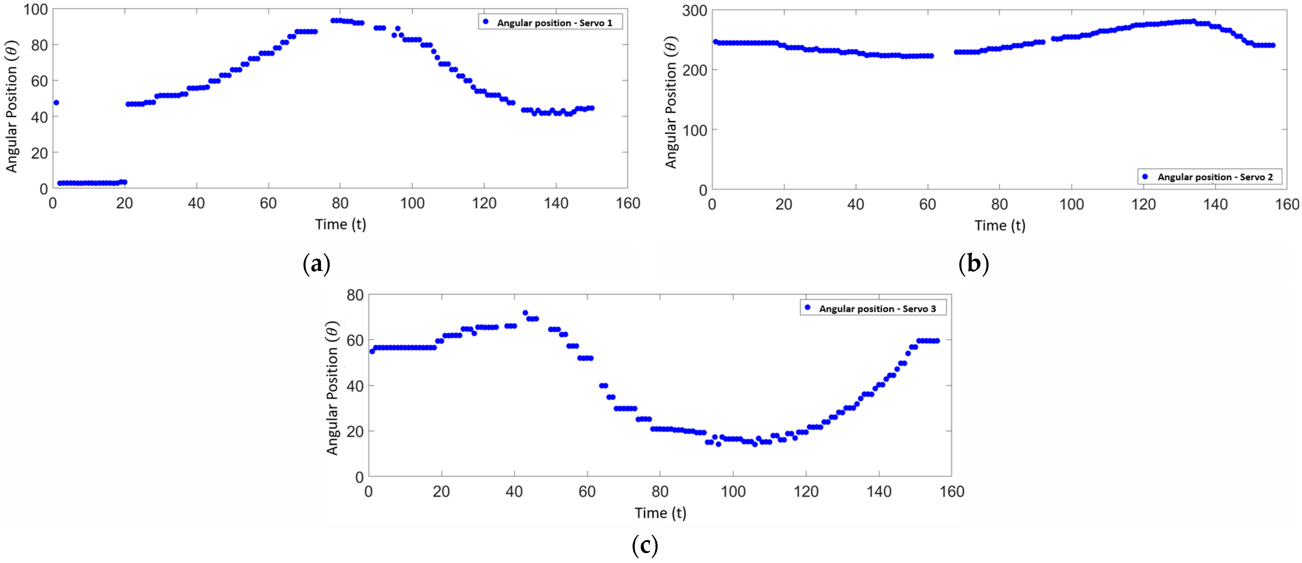
After estimating and detecting the target, the target was moved along the circular trajectory, and the angular positions were estimated. The angular results were graphed and visualized in Figure 26a–c, with 156 values obtained at a capture rate of 30 fps as a result of traveling the circular path.
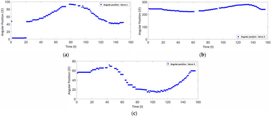
Figure 26.
(a) Angular position estimation—servomotor 1. (b) Angular position estimation—servomotor 2. (c) Angular position estimation—servomotor 3.
In this study, the movement of the object was based on the trajectory established within the manipulator work area. To validate the system performance, several trajectories were manually conducted with the vision system and the Kalman filter in operation. The gaps observed in Figure 26a,b occurred during periods when the object remained static due to manual movement. These static periods resulted in no new data points being generated, leading to the gaps visible in the plots. To provide a comprehensive evaluation of the system performance, additional data presenting the tracking error in position, velocity, and time should be included. These data will help demonstrate the precision and latency of the tracking system, offering a clearer picture of its accuracy and responsiveness.
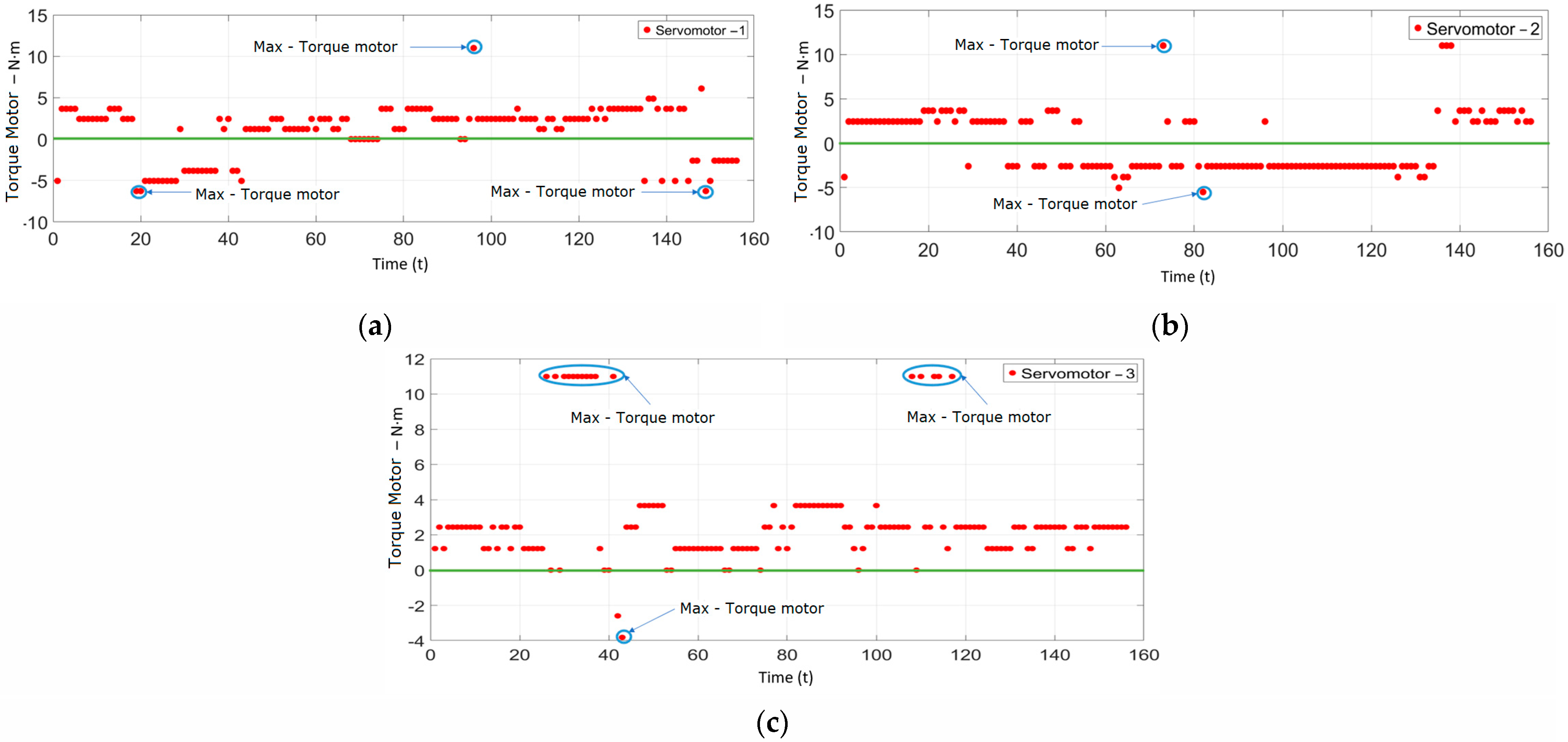
Finally, the torques delivered by the servomotors were recorded when detecting and estimating the target coordinates, as shown in Figure 27a–c. These data illustrate the maximum or critical points where the links reach their limits within the work area.

Figure 27.
(a) Estimation of motor torque—servomotor 1. (b) Motor torque estimation—servomotor 2. (c) Motor torque estimation—servomotor 3.
For future work, it is proposed to calculate and analyze the dynamic equations of the 3-RRR kinematic chain parallel manipulator using the Lagrange method to study the torques in the kinematic chains. Advanced control methodologies, such as coupled PID or control based on state variables, could be applied to improve the control of kinematic chains. Additionally, the vision system could be enhanced by applying stereo vision, which would expand the field of view from different angles and allow better object detection, applying methodologies such as RANSAC and SURF to compare results. Finally, machine learning methodologies could be implemented, such as deep neural networks, for the estimation and detection of objects in the vision area.
In the current phase of the study, the control system utilizes Inverse Kinematics (IK) without incorporating the dynamic model described in Section 2.3. The dynamic model was included to outline potential future work where advanced control techniques, such as those based on the dynamic model, could be implemented to further improve system performance. This future work could integrate the dynamic model into the control system to enhance the precision and responsiveness of the manipulator under various operating conditions.
It is also suggested to empirically estimate and calibrate the parameters and in the Kalman filter to achieve an optimal balance between confidence in the system model and the measurements provided by the sensor. This empirical estimation can begin with a trial-and-error phase to adjust these parameters based on historical data and the specific characteristics of the system, ensuring accurate and reliable predictions.
To further enhance the precision of tracking and reduce the delay in object following, the application of advanced control systems and the unification of the manipulator’s dynamics are recommended. These improvements would allow for the initialization of more accurate control data for the Kalman filter, potentially leading to better performance in real-time applications.
Finally, the contribution of this work addresses the integration of vision systems in parallel manipulators, highlighting the importance of improving object detection and manipulation capabilities. This approach can enhance flexibility and precision in industrial automation. The implementation of the Kalman filter for estimating the position of moving objects, especially when they are occluded, is crucial to maintaining the continuous operation of manipulators in dynamic, unstructured environments. The study of parallel manipulators, such as the 3-RRR, and the application of advanced vision and control techniques provide a basis for future research and development in more robust and precise manipulators, with applications across various industries.
4. Conclusions
In this study, a Kalman filter was implemented to estimate the position of a moving object, particularly when occlusions occur. The initial results indicated that while the Kalman filter can provide estimations based on limited trajectory data, the precision of these estimations can be limited due to the few data points collected and the lack of a control system. The theoretical data and the data provided by the Kalman filter showed some degree of correlation, but exact similarity could not be demonstrated. This discrepancy is due to the Kalman filter’s attempts to estimate the position when the object is occluded, which generates estimated positions in the angles of the kinematic chains and similarly for the torques exerted by the servomotors.
The Eye-to-Hand configuration provided a stable and wide view of the environment, enabling robust detection and tracking of the object and the robot’s end effector. One significant advantage is the simplicity of camera calibration and mounting, as the camera did not move with the end effector of the parallel manipulator, making the system easier to implement and maintain. Additionally, applying image stabilization with homography corrected distortions and alignments in images, resulting in a more stable vision in the manipulator’s work area. However, it is important to ensure that the points used for estimating the homography are well defined, as poorly defined points can negatively affect the precision of the transformation.
The Kalman filter proved to be an essential technique for estimation and prediction in noisy dynamic systems. Its effectiveness largely depends on the accurate calibration of the and parameters. The study acknowledged that improper values for these parameters, as well as the points used for homography, could lead to system failure. The current study did not provide a comprehensive analysis of these influences, and further research is required to optimize these parameters and validate their impact on system performance.
This study not only advances the kinematic control and visual servoing fields but also opens avenues for future research, particularly in refining accuracy and extending applicability to more complex spatial manipulations. Future work could involve collecting more extensive trajectory data to improve the accuracy of the Kalman filter estimations and incorporating a control system to enhance the reliability of the results. Additionally, detailed studies on the influence of the Q and R matrices and the points for homography could be conducted to ensure robust and precise object tracking and manipulation.
Author Contributions
Conceptualization, G.C.D. and H.F.Q.; methodology, G.C.D., J.L.V., G.A.H., and H.F.Q.; software, G.C.D., J.L.V., G.A.H. and H.F.Q.; validation, G.C.D., J.L.V., G.A.H., H.F.Q. and E.A.A.; formal analysis, G.C.D., J.L.V., G.A.H., H.F.Q., E.A.A. and D.V.; investigation, G.C.D., J.L.V., G.A.H., H.F.Q. and E.A.A.; resources, G.C.D., J.L.V., G.A.H. and H.F.Q.; data curation, G.C.D., J.L.V., G.A.H., H.F.Q., E.A.A. and D.V.; writing—original draft preparation, G.C.D., H.F.Q. and E.A.A.; writing—review and editing, G.C.D., H.F.Q., E.A.A. and D.V.; visualization, G.C.D., H.F.Q., E.A.A. and D.V.; supervision, G.C.D., H.F.Q., E.A.A. and D.V.; project administration, G.C.D. and H.F.Q. All authors have read and agreed to the published version of the manuscript.
Funding
This research received no external funding.
Data Availability Statement
Data available on request from the authors.
Acknowledgments
To the Faculty of Applied Mechanics of the Technological University of Pereira.
Conflicts of Interest
The authors declare no conflicts of interest.
References
- Sahl, S.; Song, E.; Niu, D. Robust Cubature Kalman Filter for Moving-Target Tracking with Missing Measurements. Sensors 2024, 24, 392. [Google Scholar] [CrossRef] [PubMed]
- Li, Z.; Zhou, Y.; Zhu, M.; Chu, Y.; Wu, Q. Image moment-based visual positioning and robust tracking control of ultra-redundant manipulator. J. Intell. Robot. Syst. 2024, 110, 83. [Google Scholar] [CrossRef]
- Corke, P. Robotics, Vision and Control; Springer: Brisbane, Australia, 2013; pp. 450–480. [Google Scholar]
- Corke, P. Visual Control of Manipulators—A Review. In Visual Servoing; World Scientific: Singapore, 1996; pp. 1–31. [Google Scholar]
- Pulloquinga, J.L.; Ceccarelli, M.; Mata, V.; Valera, A. Sensor-Based Identification of Singularities in Parallel Manipulators. Actuators 2024, 13, 168. [Google Scholar] [CrossRef]
- Chaumette, F.; Hutchinson, S. Visual Servo Control Part I: Basic Approaches. IEEE Robot. Autom. Mag. 2006, 13, 82–90. [Google Scholar] [CrossRef]
- Corke, P.; Hutchinson, S. A New Hybrid Image-Based Visual Servo Control Scheme. In Proceedings of the Conference on Decision and Control 2000, Sydney, NSW, Australia, 12–15 December 2000; pp. 2521–2526. [Google Scholar]
- Chaumette, F.; Hutchinson, S. Visual Servo control. Part II: Advanced Approaches. IEEE Robot. Autom. Mag. 2007, 14, 109–118. [Google Scholar] [CrossRef]
- Rosenzveig, V.; Briot, S.; Martinet, P.; Ozgur, E.; Bouton, N. A Method for Simplifying the Analysis of Leg-Based Visual Servoing of parallel Robots. In Proceedings of the 2014 IEEE International Conference on Robotics and Automation (ICRA), Hong Kong, China, 31 May–7 June 2014; 2014; pp. 5720–5727. [Google Scholar]
- Hesar, M.; Masouleh, M.; Kalhor, A.; Menjad, M.; Kashi, N. Ball Tracking with a 2-DOF Spherical Parallel Robot Based on Visual Servoing Controllers. In Proceedings of the 2014 Second RSI/ISM International Conference on Robotics and Mechatronics (ICRoM), Tehran, Iran, 15–17 October 2014; pp. 292–297. [Google Scholar]
- Luo, R.; Chou, S.; Yang, X.; Peng, N. Hybrid Eye-to-hand and Eye-in-hand visual Servo System for Parallel Robot Convenyor Object tracking and Fetching. In Proceedings of the IECON 2014—40th Annual Conference of the IEEE Industrial Electronics Society, Dallas, TX, USA, 29 October–1 November 2014; pp. 2558–2563. [Google Scholar]
- Trujano, M.; Garrido, R.; Soria, A. Stable Visual Servoing of an Overactuated Planar Parallel Robot. In Proceedings of the 2010 7th International Conference on Electrical Engineering Computing Science and Automatic Control, Tuxtla Gutierrez, Mexico, 8–10 September 2010; pp. 182–187. [Google Scholar]
- Briot, S.; Martinet, P.; Rosenzveig, V. The Hidden Robot: An Efficient Concept Contributing to the Analysis of the Controllability of Parallel Robots in Advanced Visual Servoing Techniques. IEEE Robot. Autom. Soc. 2015, 31, 1337–1352. [Google Scholar] [CrossRef]
- Dallej, T.; Goutefarde, M.; Andreff, N.; Michelin, M.; Martinet, P. Towards vision-based control of cable-driven parallel robots. In Proceedings of the 2011 IEEE/RSJ International Conference on Intelligent Robots and Systems, San Francisco, CA, USA, 25–30 September 2011; pp. 2855–2860. [Google Scholar]
- Bellakehal, S.; Andreff, N.; Mezouar, Y.; Tadjine, M. Vision/force control of parallel robots. Mech. Mach. Theory 2011, 46, 1376–1395. [Google Scholar] [CrossRef]
- Traslosheros, A.; Sebastian, J.; Angel, L.; Roberti, F.; Careli, R. Visual Servoing for the Robotenis System: A Strategy for a 3 DOF Parallel Robot to Hit a Ping-Pong Ball. In Proceedings of the Decision and Control and European Control Conference (IEEE) 2011, Orlando, FL, USA, 12–15 December 2011; pp. 5695–5701. [Google Scholar]
- Luo, J.; Liu, H.; Yu, S.; Xie, S.; Li, H. Development of an Image-based Visual Servoing for Moving Target Tracking Based on Bionic Spherical Parallel Mechanism. In Proceedings of the International Conference on Robotics and Biomimetics 2014, Bali, Indonesia, 5–10 December 2014; pp. 1633–1638. [Google Scholar]
- McInroy, J.; Qi, Z. Nonlinear Image Based Visual Servoing Using Parallel Robots. In Proceedings of the International Conference on Robotics and Automation (IEEE) 2007, Rome, Italy, 10–14 April 2007; pp. 1715–1720. [Google Scholar]
- Zhang, S.; Ding, Y.; Hao, K. A Stereo-Vision Based Compensation Method for Pose Error of a 6-DOF Parallel Manipulator with 3-2-1 Orthogonal Chains. In Proceedings of the 2008 International Conference on Audio, Language and Image Processing, ICALIP 2008, Shanghai, China, 7–9 July 2008; pp. 1540–1544. [Google Scholar]
- Bouguet, J.Y. Camera Calibration Toolbox for Matlab. Available online: http://www.vision.caltech.edu/bouguetj/calib_doc (accessed on 21 February 2021).
- Tsai, R. A versatile Camera Calibration Technique for High-Accuracy 3D Machine Vision Metrology Using Off-the-Shelf TV Cameras and Lenses. IEEE J. Robot. Autom. 1987, 3, 323–344. [Google Scholar] [CrossRef]
- Zhang, Z. A flexible new technique for camera calibration. Trans. Pattern Anal. Mach. Intell. 2000, 26, 1330–1334. [Google Scholar] [CrossRef]
- Zhang, Z. Camera Calibration with One-Dimensional Objects. Trans. Pattern Anal. Mach. Intell. 2004, 7, 892–899. [Google Scholar] [CrossRef] [PubMed]
- Gonzales, J. Estudio Experimental de Metodos de Calibracion y Autocalibracion de Cámaras. Ph.D. Thesis, Universidad de las Palmas de Gran Canaria, Las Palmas de Gran Canaria, Spain, 2003. [Google Scholar]
- Matas, J.; Chum, O.; Urban, M.; Pajdla, T. Robust wide baseline stereo from maximally stable extremal region. Image Vis. Comput. 2004, 22, 761–767. [Google Scholar] [CrossRef]
- Mikolajczyk, K.; Schmid, C. An affine invariant interest point detector. In Proceedings of the Computer Vision—ECCV 2002, Copenhagen, Denmark, 28–31 May 2002; pp. 128–142. [Google Scholar]
- Lowe, D. Object Recognition from Local Scale-Invariant Features. In Proceedings of the Seventh IEEE International Conference Computer Vision, Kerkyra, Greece, 20–27 September 1999. [Google Scholar]
- Lowe, D. Distinctive image features from scale-invariant keypoints. Int. J. Comput. Vis. 2004, 60, 91–100. [Google Scholar] [CrossRef]
- Witkin, A. Scale-Space Filtering, Acoustics, Speech, and Signal Processing. In Proceedings of the International Conference on ICCASSP’84, San Diego, CA, USA, 19–21 March 1984. [Google Scholar]
- Bhattacharya, J.; Majumder, S.; Sanyal, G. The Gaussian Maxima Filter (GMF): A New Approach for Scale-Space Smoothing of an Image. In Proceedings of the India Conference (INDICON), Kolkata, India, 17–19 December 2010. [Google Scholar]
- Huynh, B.P.; Kuo, Y.L. Dynamic filtered path tracking control for a 3RRR robot using optimal recursive path planning and vision-based pose estimation. IEEE Access 2020, 8, 174736–174750. [Google Scholar] [CrossRef]
- Rybak, L.A.; Khalapyan, S.Y.; Malyshev, D.I. Optimization of the trajectory of movement of a parallel robot based on a modified ACO algorithm. IOP Conf. Ser. Mater. Sci. Eng. 2019, 560, 012036. [Google Scholar] [CrossRef]
- Gao, Y.; Chen, K.; Gao, H.; Xiao, P.; Wang, L. Small-angle perturbation method for moving platform orientation to avoid singularity of asymmetrical 3-RRR planner parallel manipulator. J. Braz. Soc. Mech. Sci. Eng. 2019, 41, 538. [Google Scholar] [CrossRef]
- Hou, Y.; Deng, Y.; Zeng, D. Dynamic modelling and properties analysis of 3RSR parallel mechanism considering spherical joint clearance and wear. J. Cent. South Univ. 2021, 28, 712–727. [Google Scholar] [CrossRef]
- Reyes-Cortés, F. Robótica: Control de Manipuladores Paralelos, Colonia del Valle; Alfaomega: Madrid, Spain, 2013; pp. 14–22. [Google Scholar]
- Cisneros, M.; Jimenez, E.; Navarro, D. Fundamentos de Robótica y Mecatrónica con MATLAB y Simulink; Alfaomega: Madrid, Spain, 2014. [Google Scholar]
- Bar-Shalom, Y.; Li, X.R.; Kirubarajan, T. Estimation with Applications to Tracking and Navigation: Theory Algorithms and Software; John Wiley & Sons: Hoboken, NJ, USA, 2001. [Google Scholar]
- Welch, G.; Bishop, G. An Introduction to the Kalman Filter; University of North Carolina at Chapel Hill, Department of Computer Science: Chapel Hill, NC, USA, 1995. [Google Scholar]
- Simon, D. Optimal State Estimation: Kalman, H infinity, and Nonlinear Approaches; John Wiley & Sons: Hoboken, NJ, USA, 2006. [Google Scholar]
- Bradski, G.; Kaehler, A. Learning OpenCV: Computer Vision with the OpenCV library; O’Reilly Media: Newton, MA, USA, 2008. [Google Scholar]
- Corke, P. Robotics, Vision and Control: Fundamental Algorithms in MATLAB®; Springer: Berlin/Heidelberg, Germany, 2023. [Google Scholar]
- Chui, C.K.; Chen, G. Kalman Filtering with Real-Time Applications; Springer: Berlin/Heidelberg, Germany, 2017. [Google Scholar]
- Maybeck, P.S. Stochastic Models, Estimation, and Control; Academic Press: Cambridge, MA, USA, 1979. [Google Scholar]


Disclaimer/Publisher’s Note: The statements, opinions and data contained in all publications are solely those of the individual author(s) and contributor(s) and not of MDPI and/or the editor(s). MDPI and/or the editor(s) disclaim responsibility for any injury to people or property resulting from any ideas, methods, instructions or products referred to in the content. |
© 2024 by the authors. Licensee MDPI, Basel, Switzerland. This article is an open access article distributed under the terms and conditions of the Creative Commons Attribution (CC BY) license (https://creativecommons.org/licenses/by/4.0/).