Abstract
Wavefront Coding (WFC) is an innovative technique aimed at extending the depth of focus (DOF) of optics imaging systems. In digital imaging systems, super-resolution digital reconstruction close to the diffraction limit of optical systems has always been a hot research topic. With the design of a point spread function (PSF) generated by a suitably phase mask, WFC could also be used in super-resolution image reconstruction. In this paper, we use a deep learning network combined with WFC as a general framework for images reconstruction, and verify its possibility and effectiveness. Considering the blur and additive noise simultaneously, we proposed three super-resolution image reconstruction procedures utilizing convolutional neural networks (CNN) based on mean square error (MSE) loss, conditional Generative Adversarial Networks (CGAN), and Swin Transformer Networks (SwinIR) based on mean absolute error (MAE) loss. We verified their effectiveness by simulation experiments. A comparison of experimental results shows that the SwinIR deep residual network structure based on MAE loss optimization criteria can generate more realistic super-resolution images with more details. In addition, we used a WFC camera to obtain a resolution test target and real scene images for experiments. Using the resolution test target, we demonstrated that the spatial resolution could be improved from 55.6 lp/mm to 124 lp/mm by the proposed super-resolution reconstruction procedure. The reconstruction results show that the proposed deep learning network model is superior to the traditional method in reconstructing high-frequency details and effectively suppressing noise, with the resolution approaching the diffraction limit.
1. Introduction
In digital imaging systems, providing a sharp image with a higher imaging frame rate is often desired [1,2,3]. However, in conventional optical imaging system, the quality of an image rapidly degrades when the object deviates from the focal plane. Conversely, constrained by the transmission bandwidth of the detector, increasing the frame rate is commonly achieved through two methods, but one involves sacrificing field of view, while the other entails sacrificing detector resolution. The approach of sacrificing field of view involves cropping the image and only outputting part of the field of interest (sub-sampling) [4,5,6]. This method reduces the field of view range and has significant limitations in its application. The approach of sacrificing resolution is to extract specific pixel output (skipping) [7], which maintains the field of view while resulting in a significant reduction in image details [8]. In addition, there exists another application scenario in which the ambient illumination is low. To maintain the frame rate without reducing it, it is necessary to expand the size of the photosensitive pixel. The detector operates in the binning mode, where the current responses of adjacent photosensitive units are added together and merged for output, at which point the imaging resolution is reduced. Both operational modes will result in a substantial loss of information in the image, so the reconstruction of high-resolution details based on low-resolution images holds immense significance in practical applications [9,10,11].
The question of how to break through the diffraction limit of optical systems and achieve super-resolution has always been a research hotspot in academic circles. In the microscopy field [12,13,14,15], super-resolution fluorescence microscopy technology [16,17], which utilizes quenching fluorescent molecules and the principle of quenching by stimulated radiation, has broken through the diffraction limit that conventional optical microscopes cannot reach, achieving clear observation of biological structures within 200 nm.
With the development of computer technology and image processing techniques, super-resolution is no longer referred to as exceeding the physical diffraction limit [18,19]. In fact, in numerous imaging fields, the pixel size of the detector is still insufficient to reach the diffraction limit of the optical system. Despite the rapid development of the CMOS process in recent years, the physical size of pixels has become progressively smaller, which will result in a significant increase in noise. Improving the resolution while maintaining the size of the pixels holds significant research value. The significance of super-resolution is not only to expand the size of the image but also more importantly to enhance the details that are not present in low-resolution images. Methods for achieving super-resolution consist of multi-frame reconstruction [20,21] and single-frame reconstruction [22]. The multi-frame super-resolution technique reconstructs the details of a high-resolution image by inputting a series of low-resolution images with sub-pixel shifts and using the complementary information between the low-resolution images. Typical algorithms are the iterative back-projection method [23,24] and convex set projection method. Single-frame image super-resolution reconstruction obtains a high-resolution image by inputting a single-frame low-resolution image after some mapping relationship, which is more challenging due to the absence of complementary information. Currently, single-frame super-resolution reconstruction is mainly realized through two types of methods, namely interpolation-based methods [25] and learning-based methods [26]. Interpolation-based methods include nearest neighbor interpolation, bi-linear interpolation, and bi-cubic interpolation. These methods are applied to expanding image size, but only improve the visual effect of the image without enhancing the image details.
Learning-based methods establish the relationship between low- and high-resolution mapping by training on numerous pairs of low- and high-resolution image samples [27]. The classical method is the super-resolution reconstruction method based on sparse representation [28], which constructs the low- and high-resolution images as an over-complete dictionary during the learning process, and first obtains the sparse representation coefficients of the low-resolution image during the inference process, and then unites the over-complete dictionary of the high-resolution image to obtain the high-resolution image. This method has a strong ability to enhance details, but is limited by sparse expression capabilities and is still a shallow learning method. In recent years, deep learning networks have made substantial advances in many computer tasks, such as image classification [29,30], object detection [31,32], and semantic segmentation [33,34]. Furthermore, Li et al. [35] established links between an interpolated low-resolution image and a super-resolution image using a Hierarchical Swin Transformer (HST) network. Da et al. [36] proposed a channel attention residual enhanced Swin Transformer denoising network (CARSTDn) for image denoising. In infrared polarization imaging, Ma et al. [37] proposed an infrared polarization super-resolution reconstruction detection system based on sparse representation with the Micro-scanning Polarization Projection on Convex Sets (MPPOCS) algorithm to address pseudo-polarized information, image downsampling and mosaicking. For deblurring, Kong et al. [38] showed an improvement compared to other works.
In our work, we propose a method for super-resolution degraded imaging reconstruction by wavefront coding (WFC) technology and deep learning networks. Under the condition of detector downsampling output, super-resolution image reconstruction is achieved through deep learning networks based on the high-resolution point spread function (PSF) in an WFC imaging system. We use three representative deep learning networks to simulate the performance of the super-reconstruction algorithm on the impacts of mean square error (MSE) loss [39], perceptual loss [40], and mean absolute error (MAE) loss [41]. Firstly, we perform a comparative analysis for two convolutional neural network (CNN) structures with different depths. Then, we compare the transformer network structure based on MAE with the neural network structures. Finally, through simulation experiments and real scene reconstruction experiments combined with an actual wavefront coding system, we find that the transformer network structure based on MAE performs the best, also validating the effectiveness of the super-resolution reconstruction method.
2. Wavefront Coding Super-Resolution Reconstruction Principle
Wavefront coding is a depth-of-focus (DOF) technology combining optical coding and digital image processing. The wavefront of the optical system can be coded and modulated by placing a specially designed phase mask at the exit pupil of the optical system, so that the system generates a focus-invariant PSF and optical transfer function (OTF). In the magnitudes of OTFs (MTFs), the cut-off frequency corresponding to the diffraction limit represents the system’s maximum resolving ability. The WFC system ensures that the MTF become almost invariant regardless of the defocus value without any zeros, providing the necessary information closer to the cut-off frequency for super-resolution reconstruction. The process of obtaining coded images can be expressed as:
where denotes the encoded and captured intermediate image, denotes the original high-resolution image, h denotes the acquired PSF, “*” denotes the convolution operation, N denotes Gaussian noise, and “” indicates downsampling.
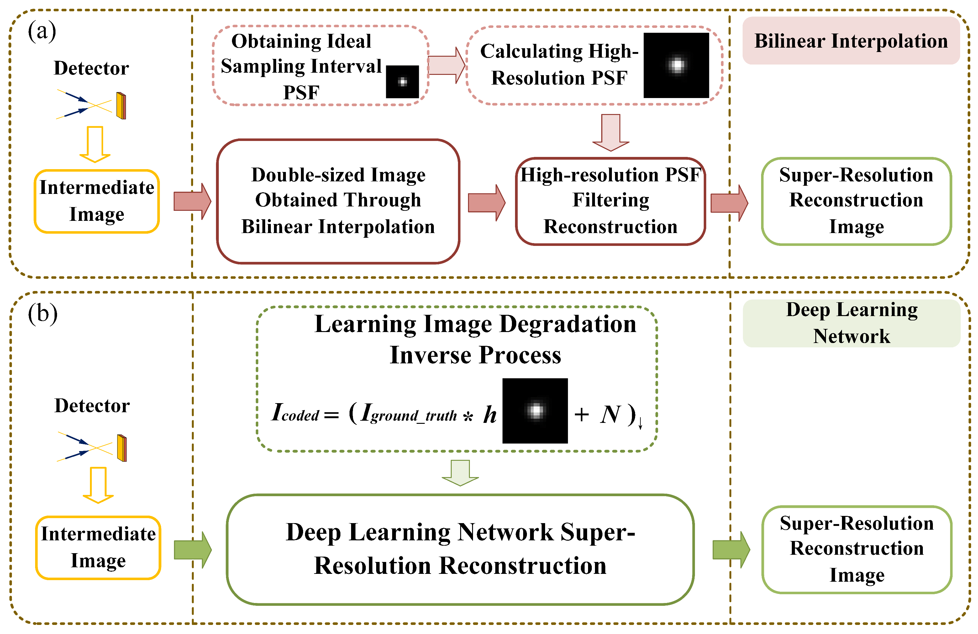
To demonstrate that a wavefront coding system combined with a deep learning network can be effectively applied to super-resolution reconstruction, we utilized a visible light lens–combined WFC imaging system [42] meticulously designed by our team. Diagrams of a traditional imaging system and a WFC system, and the corresponding MTFs with different image distance are presented in Appendix A. As can be seen from Figure A1c, the MTF analysis reveals that the cut-off frequency of traditional imaging systems is significantly lower than the diffraction limit, resulting in a substantial loss of imaging information, which seriously affects imaging quality. In contrast, though the MTFs of the WFC system are approaching zero with increasing frequency and at much lower frequencies than with the traditional lens, the system contains no zero-frequency response. Additionally, as the object distance deviates from the optimal focus position, the amplitude of the curve does not change significantly. This consistency provides better conditions for subsequent super-resolution reconstruction. Figure 1 provides a schematic of super-resolution reconstruction with the WFC system (optical encoding procedure) and computational imaging (digital decoding procedure). A phase mask is placed at the pupil position of the optical system, thereby the system produces focus invariant OTFs and sampled PSFs. The intermediate images are captured by the detector and downsampled, which can be reconstructed via a digital procedure using the sampled PSFs.
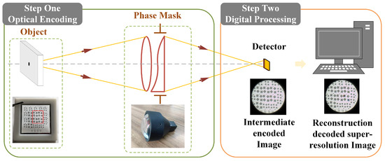
Figure 1.
Wavefront coding system schematic diagram.
Currently, there is limited exploration of super-resolution techniques in the field of wavefront coding [43,44]. Conventional optical systems are optimized so that the aberration is suppressed to the minimum state. When the physical size of the pixel is lower than the theoretical limit of the resolution of the optical system, the system operates in an undersampling state, resulting in signal aliasing. In the wavefront coding system, the MTF decreases, and PSF dispersion size undergoes expansion, thus effectively reducing the aliasing effect. According to the above theoretical analysis, the PSF corresponding to the detector sampling interval is tentatively referred to as the low-resolution PSF, and the PSF corresponding to half the size of the sampling interval is called as the high-resolution PSF. The wavefront coding super-resolution decoding technique can be implemented by the process shown in Figure 2a. If the high-resolution PSF is directly used to filter the low-resolution intermediate image, the image will produce a very severe ringing effect. Therefore, it is necessary to first interpolate the low-resolution image to a resolution twice the original resolution, both horizontally and vertically. Afterward, the image can be restored to a high-resolution image through Wiener filtering [45] and other methods [46].
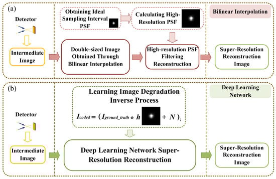
Figure 2.
Super-resolution and low-resolution PSF measurements by (a) bi-linear interpolation and (b) deep learning network.
We propose a method to increase the imaging frame rate based on the above wavefront coding super-resolution theory combined with the designed large-aperture wavefront coding system [42]. By making the detector operate in the downsampling mode, the horizontal and vertical resolution of the image is 1/2 of the original, and the total number of pixels is 1/4 of the original, compared with the full-pixel output mode. The PSF of the central field of view at the optimum viewing distance is measured, and the PSFs of the full-pixel and the downsampling are obtained, respectively, as shown in Figure 2a.
In this paper, we use the PSF of the actual system as the prior of blurring for reconstruction simulation and a deep learning network to replace the bi-linear interpolation process in Figure 2a. In order to improve the operation efficiency of the algorithm, the processes of super-resolution and image decoding are merged to achieve end-to-end super-resolution reconstruction, so that the network inputs the low-resolution coded image and outputs the super-resolution reconstruction image directly. This process is shown in Figure 2b. During this process, the deep learning model is trained to learn the degradation process of the ground truth image as described in Equation (1). This enables the network to reconstruct clearer images from low-resolution encoded images. Compared with the conventional super-resolution tasks, the network is not only responsible for image resolution enhancement, but also for image decoding.
3. Super-Resolution Reconstruction Deep Learning Network
For the task of image reconstruction, deep learning networks have shown excellent performance for image denoising and blind deblurring. In order to learn the mapping F from observed image to ground truth , the architecture of super-resolution reconstruction mainly consists of three operations: patch feature extraction, non-linear transformation, and reconstruction. The wavefront coding process can be simulated by blurring the PSF and adding noise, and downsampling the blurred image simulates the downsampling process of the detector. The downsampling blurred image is used as the low-resolution intermediate image input to the network, with the original prior-PSF blurred image as the output ground-truth image.
In order to test various super-resolution reconstruction algorithms based on deep learning networks, we tried three network structures. The first is super-resolution CNN (SRCNN), a convolutional neural network based on MSE loss with fewer network layers. The second network structure is super-resolution GAN (SRGAN), a generative adversarial network based on perceptual loss with a relatively complex network. The last network structure is image reconstruction Swin Transformer (SwinIR), a Swin Transformer network based on MAE loss with more complex network architecture and more parameters.
3.1. Convolutional Neural Network Based on MSE Loss
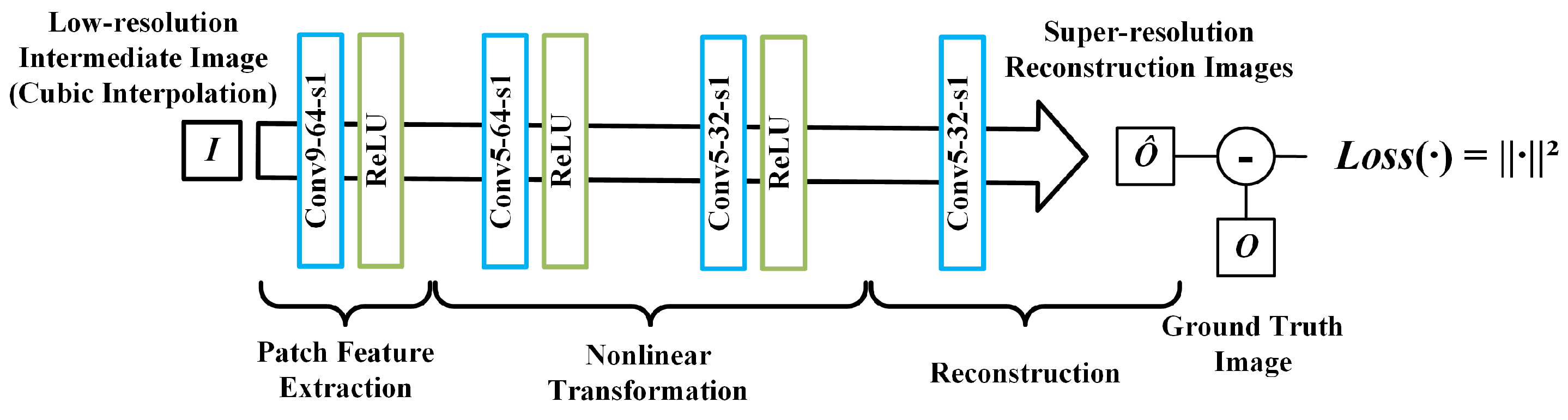
The SRCNN is of great significance in super-resolution algorithms, inspiring many subsequent approaches. The network achieves super-resolution reconstruction through three convolutional layers, where each convolutional layer corresponds to a stage in the reconstruction process, namely the block feature extraction, nonlinear mapping, and reconstruction stages. The network structure is shown in Figure 3. Taking the first layer Conv9-64-s1 as an example, this indicates that the convolution kernel size of the convolution layer is 9, the number of feature layers is 64, and the convolution step size is 1.
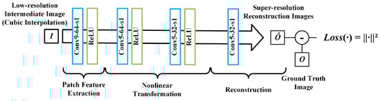
Figure 3.
The structure of the super-resolution convolutional neural network.
In the block feature extraction stage, a series of convolution kernels is used to extract features from low-resolution images and convert them into abstract features, where the feature layer can be represented as:
where and represent the convolution and bias of the i-th filter, the symbol ∗ is the convolution, and f is the nonlinear activation function, here, using a nonlinear rectification unit (ReLU) [47]. For single-channel image input, each convolution kernel has a spatial size of , and the output contains feature layers equal to the number of convolutional layers.
After feature layer extraction, these features need to be converted to higher dimensions through nonlinear mapping. This process can be expressed as:
Assuming that there are high-dimensional feature layers in total, and the convolution kernel has a single-dimensional space size of . Then, according to the size of , the nonlinear mapping can be classified into two types: when is equal to 1, this transformation can be interpreted as a single-pixel mapping; and when is greater than 1, the receptive field of the convolution is broadened and the influence of adjacent pixels is introduced into the transformation. Therefore, any number of convolutional layers can be added during this stage, and the number of convolution parameters between the layer and the layer is .
In the reconstruction stage, the high-dimensional features need to be converted into super-resolution images, and the process can be expressed as:
where is the final predicted image. Unlike the previous two stages, the convolution in this stage does not require a nonlinear activation function, so the reconstruction process is more like a weighted average of high-dimensional features. Assuming that the final output is a single-channel image, the number of convolution parameters in this process is .
In addition to the three-layer convolution structure, we add a convolution layer (the second convolution layer in Figure 3 in the nonlinear mapping stage to determine the impact of network depth on the super-resolution results. Including the bias parameters, SRCNN-915 with the three-layer convolutional structure contains 8129 parameters, while SRCNN-9515, with a convolutional layer added, contains 110,593 parameters, which is 13.6 times that of SRCNN-915.
In the training stage, the network needs to learn the mapping relationship from the low-resolution intermediate image to the ground-truth image. Assuming that the parameters to be learned by the network are denoted as , , the loss function of the network is defined as the Euclidean distance between the network output and the ground-truth image, which is MSE. The network is trained with the aim of minimizing the loss function. The process can be expressed as:
where N is the number of training patches.
3.2. Conditional Generative Adversarial Network Based on Perceptual Loss
The second super-resolution reconstruction algorithm used is a generative adversarial network (GAN), or more precisely a conditional generative adversarial network (CGAN). A traditional GAN contains a generative network and a discriminative network. The generative network needs to learn the mapping relationship from the noisy image to the real image, while the discriminative network needs to discriminate the difference from the output of the generative network and ground-truth. Through alternate training, the generative network and the discriminative network continue to “evolve”, and eventually output a “false” image that is very close to the real image. Based on the principle of GANs, the input of CGAN is not limited to a noisy image, it can be a blurred or low-resolution image, and the network eventually outputs a super-resolution image.
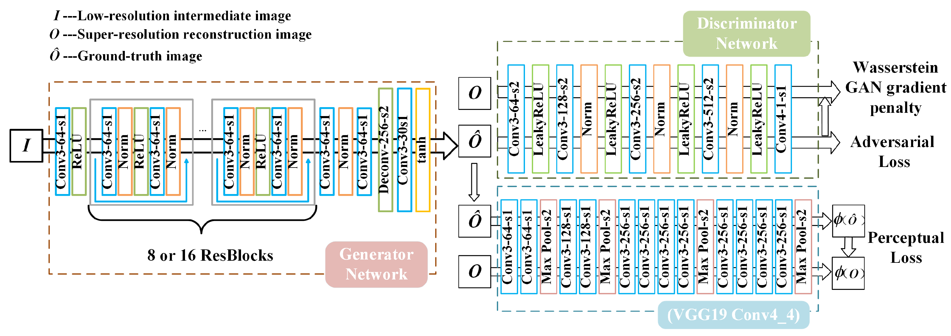
We employ a generative network containing several convolutional layers and residual blocks [48], which is shown in Figure 4. The final stage of the network contains an inverse convolutional layer to achieve the image resolution improvement, and the last activation function is tanh, which maps the output to between (−1, 1). To test the impact of network depth on the super-resolution reconstruction results, we reduced the number of residual blocks in the generative network from 16 (SRGAN-16ResBlocks) to 8 (SRGAN-8ResBlocks). This modification resulted in 780,739 parameters after the reduction, which is almost half of the initial parameter count of 1,374,659.
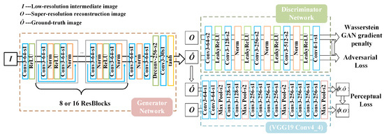
Figure 4.
The structure of the super-resolution generative adversarial network.
The loss function of the generation network consists of three parts, consisting of an MSE, auxiliary training network, and discriminant network, respectively, expressed as:
where MSE represents the pixel difference between the generated image and the ground-truth image. The VGG loss provided by the auxiliary training network is also referred to as the perceptual loss, which is defined as the Euclidean loss between the feature representations of a decoded image and the reference image O:
where represents the feature map of the j-th layer convolution before the i-th maximum pooling layer in the VGG19 network structure. Both i and j are used as 4 in this study. The incorporation of perceptual loss enhances the realism of the style and texture of the generated image. The loss provided by the discriminant network is the Wasserstein distance, defined as:
where and describe parameters in the discriminator and generator, respectively, and N denotes the number of training samples. The discriminatory network adopts the structure proposed in the literature, comprising five convolutional layers. To avoid the issue of gradient disappearance or explosion in WGAN (Wasserstein GAN) during training, the loss of the discriminator adopts the WGAN-GP form, denoted as:
where denotes the distribution of the real data, denotes the distribution of the output data of the generative network, and denotes the randomly interpolated sampling on the line connecting and , that is .
3.3. Swin Transformer Based on MAE Loss
The third super-resolution reconstruction algorithm used is the shifted windows version of the hierarchical vision transformer (Swin Transformer), known as SwinIR. The Swin Transformer utilized in the algorithm is based on the standard multihead self-attention of the original Transformer layers, which integrates the advantages of both CNN and Transformer, and demonstrates tremendous potential for various applications. On the one hand, it has the advantage of CNN of being able to process images of large size due to the local attention mechanism, while, on the other hand, it has the advantage of Transformer of being able to model long-range dependence with the shifted window scheme.
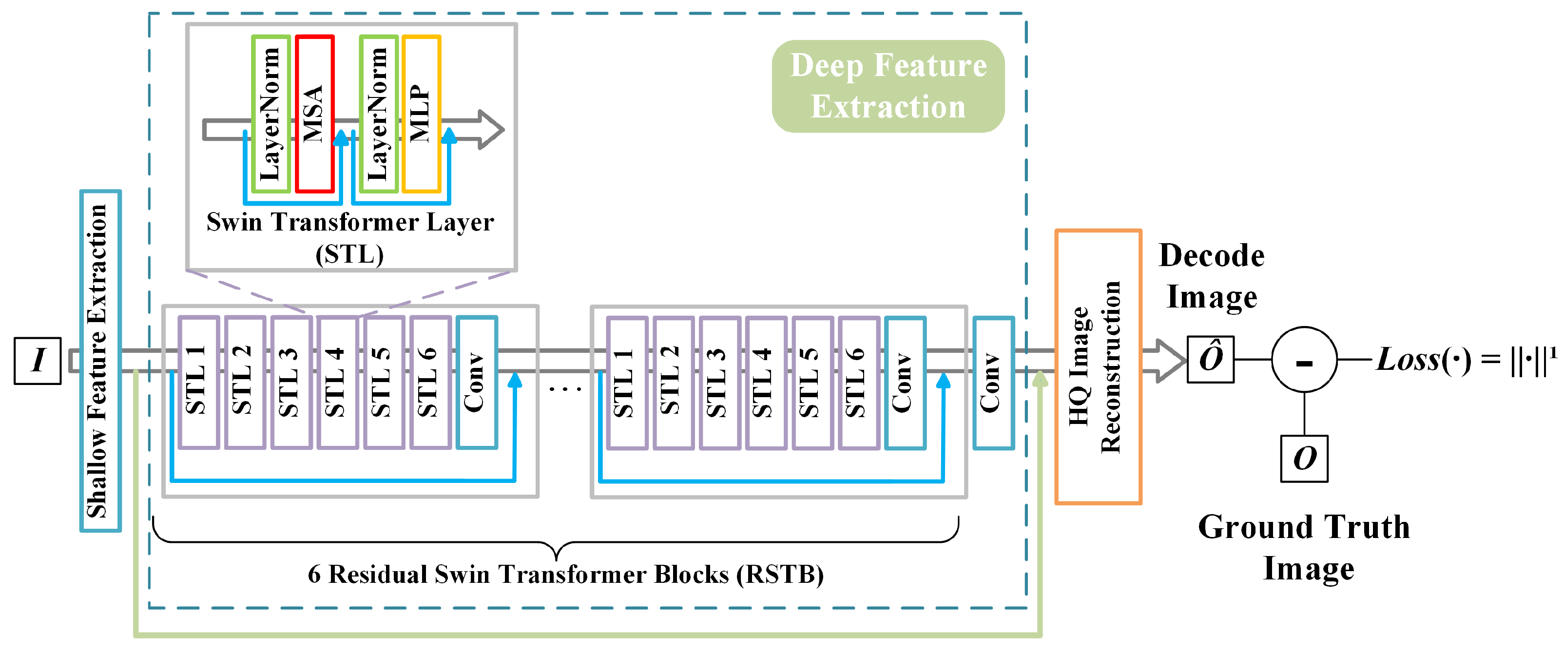
The model mainly consists of three components, namely the shallow feature extraction, deep feature extraction, and high-quality image reconstruction modules. The deep feature extraction module is primarily composed of residual Swin Transformer blocks (RSTBs), where each RSTB contains multiple layers of Swin Transformers for local attention and cross-window interaction. Additionally, a convolutional layer is appended at the end of each block for feature enhancement, while residual connections are used to facilitate the aggregation of features. Finally, shallow and deep features are fused in the reconstruction module to achieve high-quality image reconstruction. The structure of the network model used in this paper is shown in Figure 5. The deep feature extraction module of the model includes 6 RSTBs and a convolutional layer, in which each RSTB is a residual block composed of several Swin Transformer layers (STL) and a convolutional layer.

Figure 5.
The structure of the SwinIR network.
In the shallow feature extraction stage, shallow feature extraction is performed for three parameters: image height, and width and number of input channels of the input low-resolution blur image, and this process can be expressed as:
where and , represent the low-resolution image and a convolutional layer used for shallow feature extraction, respectively, and the symbol ∗ is the convolution. Subsequently, the intermediate features are extracted block by block from the shallow features and then outputted, this process can be expressed as:
where denotes the RSTB, while represents the final convolutional layer. The incorporation of a convolutional layer at the end of feature extraction can bring the inductive bias of the convolution operation into the Transformer-based network, and establish a better foundation for the later aggregation of shallow and deep features. Furthermore, within each RSTB, which comprises six STLs and a convolutional layer, and the process of extracting intermediate features from the six STLs for a given RSTB with input feature can be expressed as:
where represents the STL in the RSTB. Then, a convolutional layer is added before the residual join. This process can be denoted as:
where is the convolutional layer in the RSTB.
In an STL, the attention function is executed for h times in parallel, and the results are concatenated to establish multihead self-attention (MSA). Then, a multi-layer perceptron (MLP) is used for further feature transformations, which contains two fully connected layers with GELU non-linearity between them. LayerNorm (LN) layers are added before both the MSA and MLP, and residual connections are used for both modules. The whole process can be represented as:
where X and Y denote the input features and output features of each STL, respectively. Finally, once the deep features have been extracted, the deep features and shallow layers of the image are upsampled and adjusted for aggregation through sub-pixel convolutional layers in the reconstruction module to reconstruct a high-quality image.
In the training stage, the network uses the L1 pixel loss in the selection of the loss function, which measures the average absolute difference between each pixel value in the generated image and the corresponding pixel value in the target image, also known as MAE. The L1 pixel loss is a more widely used loss function in image super-resolution, and the network is trained with the aim that the generated image needs to be as same as possible as the target image. The process can be expressed as:
where N is the number of image pairs used in each iteration of training as above.
4. Simulation and Imaging Experiment
The dataset is a crucial factor in assessing the effectiveness of deep learning networks. After comprehensive consideration of the quality and quantity of images in each dataset, we finally selected the DIV2K data set [49], which contains 800 training images and 100 testing images, all of which have a resolution of 2K. For the generation of the training set, the wavefront coding process can be simulated by blurring the known PSF and adding noise. The downsampled blurred image is used as the low-resolution intermediate image input to the network.
4.1. Super-Resolution Reconstruction Simulation Model
For the SRCNN structure, we discretely sampled 800 original high-definition images from the DIV2K dataset at 100 pixels intervals, obtaining a total of 235,904 image pairs. The batch input for a single iteration contains 128 image pairs for a total of 2 million iterations, which is equivalent to 1000 epochs of training on the training set. Stochastic gradient descent (SGD) and momentum methods are used for training, with the learning rate set to 0.0001. Training on the Titan-XP GPUs required a total of approximately 12 h for the SRCNN-915 structure and 34 h for the SRCNN-9515 structure.
For the SRGAN structure, in each training, a ground-truth image of 384 × 384 size is intercepted from the 2K large image, and the input is a degraded image with a size of 192 × 192 at the corresponding location. The input for a single iteration contains four image pairs and is trained on the training set for 1000 epochs using the Adam optimizer with the learning rate set to 0.0001 for the first 500 cycles and 0.00001 for the last 500 cycles. Training on the Titan-XP GPUs required a total of approximately 46 h for the SRGAN-8ResBlocks structure and 58 h for the SRGAN-16ResBlocks structure.
For the SwinIR structure, images of 96 × 96 size were intercepted from the 2K large image for each training, while the input size of the low-resolution degraded image was 48 × 48. The input for a single iteration contained three to four image pairs, which were trained for 1000 epochs on the training set using the Adam optimizer with the learning rate set to 0.002. Unlike the previous training equipment, the SwinIR structure was trained by a 3060ti GPU, requiring 91 h for training. However, as the training performance under 1000 epochs was not satisfactory, subsequent experiments opted for a model trained for 3000 epochs for analysis and comparison.
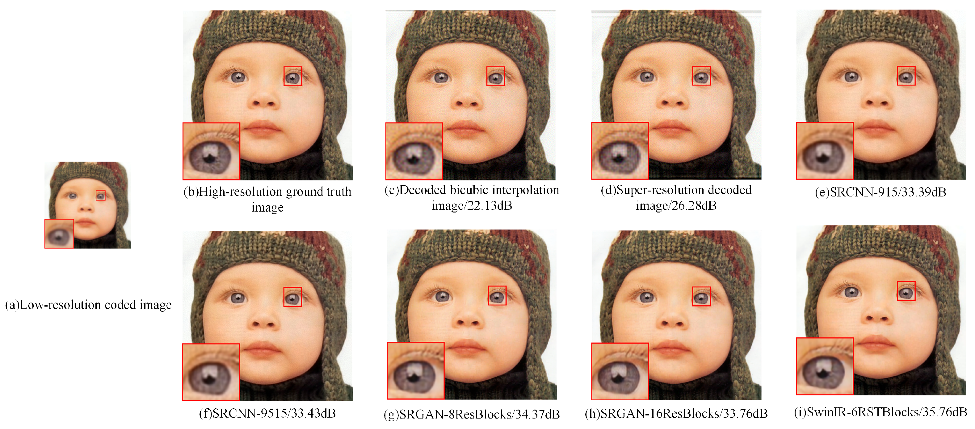
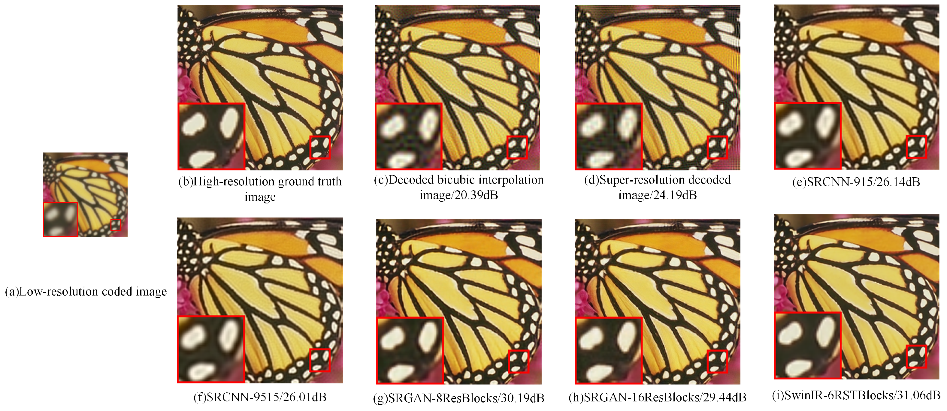
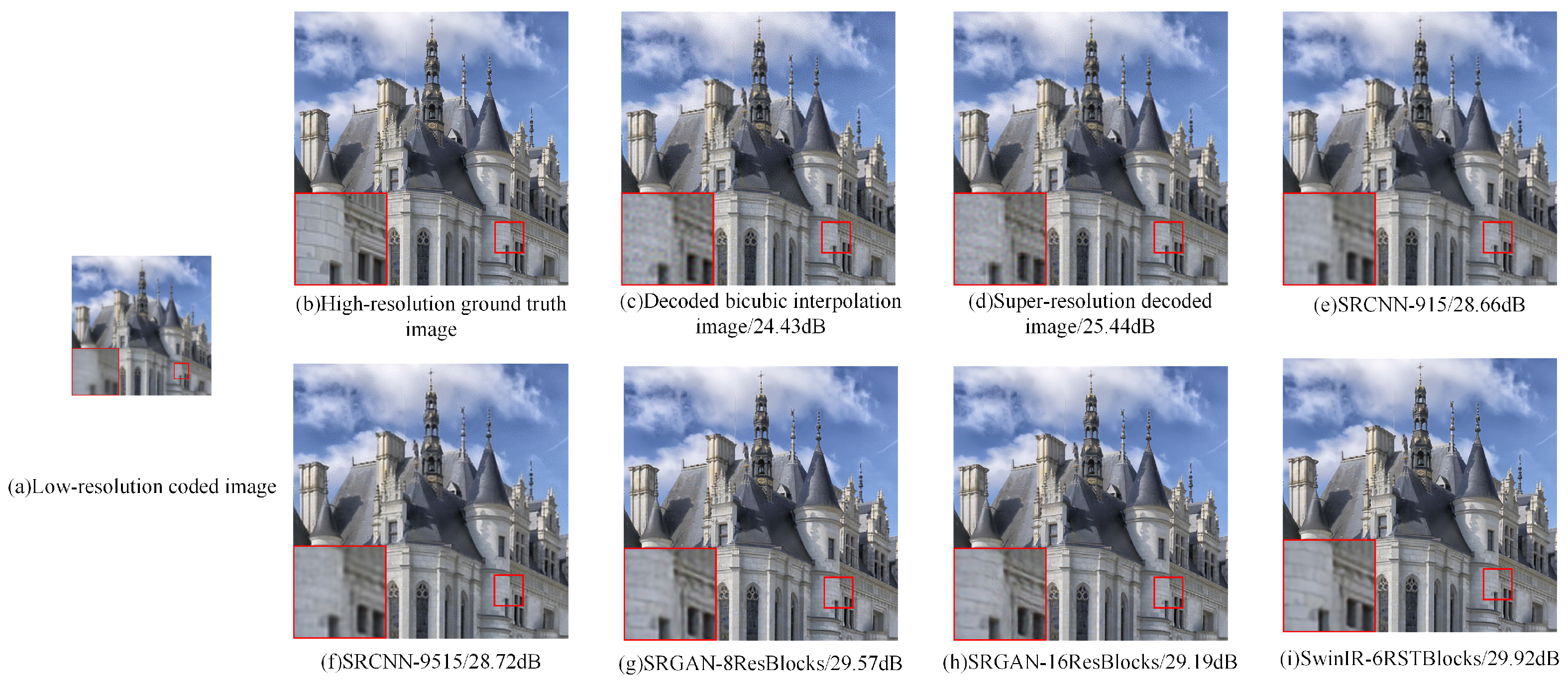
After completing the network training, we validated the network’s results on three test sets, namely Set 5, Set 14 [50], and DIV2k-Valid. For comparison, we adopted the Wiener filtering method to decode the low-resolution coded image and adopted the method in the literature [51] for super-resolution decoding. The method employed in the literature [51] involves interpolating the low-resolution intermediate coded images to obtain images with both horizontal and vertical resolutions twice that of the original. Subsequently, super-resolution decoding is performed using Wiener filtering in conjunction with the PSF of the wavefront coding system. The final reconstruction results are shown in Figure 6, Figure 7 and Figure 8. For each figure, (a) displays the low-resolution ground-truth image, (b) displays the low-resolution coded image, (c) displays the image that directly decodes a low-resolution coded image, (d) displays the super-resolution decoded image generated Wiener filtering method referred in the literature [51], (e) and (f) denote the super-resolution reconstruction results based on the SRCNN network, (g) and (h) represent the super-resolution reconstruction results based on the SRGAN network, and (i) represents the super-resolution reconstruction results based on the SwinIR network.
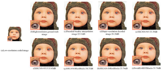
Figure 6.
Comparison of super-resolution reconstruction results (image I).

Figure 7.
Comparison of super-resolution reconstruction results (image II).
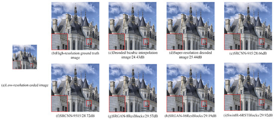
Figure 8.
Comparison of super-resolution reconstruction results (image III).
Comparing the results, it can be seen that the signal-to-noise ratio of the image generated by the super-resolution decoding algorithm in the literature [51] is marginally higher than that of the low-resolution decoded image, but the improvement effect is not obvious, as numerous details of the image are submerged in the noise. Overall, the super-resolution reconstruction effect using deep learning networks is superior. The reconstruction effect of SRCNN tends to retain a certain degree of blur in the images, and the edges are not sharp enough. In comparison, the reconstructed images based on the SRGAN network has richer details and more realistic subjective feeling. A comparison of the results obtained from different network depths indicates that the network depth has little impact on the results in the SRCNN network structure, while in the SRGAN network, increasing the network depth can bring more details to the images.Furthermore, the reconstructed image based on the SwinIR network exhibits a higher signal-to-noise ratio compared to the SRGAN network structure, while the edge artifacts of the reconstructed images are better eliminated and the details are closer to the original image.
The super-resolution reconstruction images from the three test sets were quantitatively analyzed by peak signal-to-noise ratio (PSNR) and structural similarity (SSIM), respectively, and the results are shown in Table 1. A comparison shows that the signal-to-noise ratio of the super-resolution restored images based on the deep learning network is much higher than that of the interpolation method and the method adopted in the literature [51]. Among them, SRGAN-8ResBlocks performs the best on SSIM with an average enhancement of 0.1424 compared to the method in the literature [51], while SwinIR-6RSTBlocks exhibited the greatest performance on PSNR with an average enhancement of 8.4 dB compared to the method adopted in the literature [51]; however, this network has an average enhancement on SSIM of only 0.103.

Table 1.
Peak signal-to-noise ratio (dB) and structural similarity of super-resolution reconstruction images.
Comparing the different network depths, the addition of one network layer in the SRCNN structure does not significantly impact the PSNR results, while in the SRGAN structure it can be detected that the signal-to-noise ratio of the 16-residue block is worse than that of the 8-residue block, which seems to be inconsistent with the subjective perception, and this phenomenon has also been mentioned in the literature [48]. The reason for this phenomenon may be that the network trained based on perceptual loss introduces some “false” components during the reconstruction process and these “false” texture details can be more pleasing to the human visual perception system. However, analysis of the pixel values indicates that the “false” information results in an amplification of the difference between the reconstructed image and the real image. Therefore, the performance evaluation based on PSNR does not entirely correspond to the subjective experience. Compared to the SRGAN network structure with the 8-residue block, the SwinIR structure is capable of further enhancing the PSNR while significantly reducing the presence of “false” texture details, thereby narrowing the gap between the reconstruction image and the real image.
Next, we input a color image with a resolution of 2040 × 1536 and tested the running time of the four convolutional neural networks on the Titan-XP GPU and the results are shown in Table 2. The reconstruction algorithm based on the SRCNN-915 network structure has a shorter running time of about 0.02 s, and the time is prolonged to three times of the original after adding one layer of network depth, so this network structure is suitable for the case of high real-time requirements; in contrast, the running time based on the SRGAN-8ResBlocks network structure is longer, taking about 1.2 s, and the time is about 1.5 s after increasing the network depth, so this network is more suitable for offline processing. The training equipment for the SwinIR-6RSTBlocks network structure differs from the four aforementioned convolutional neural networks. Due to the limited memory resources available on the training devices, adjustments to the network hyperparameters have a discernible impact on the network operational speed. Thus, testing SwinIR on a color image with a resolution of 1040 × 768 still results in a relatively lengthy running time, approximately 3.3 s. Nevertheless, this network is equally suitable for offline processing.
Table 2.
Comparison of the runtimes of super-resolution reconstruction algorithms using deep learning networks.
4.2. Super-Resolution Image Reconstruction Experiment
Based on the previous simulation experiments and the correlation between the reconstruction results and the running time, we finally selected the SRGAN-8ResBlocks network structure and SwinIR-6RSTBlocks network structure as the super-resolution reconstruction algorithms for real imaging.However, since the two networks have their own advantages in terms of PSNR and SSIM performance evaluations, it is necessary to combine them with a real-world scene for comparative analysis in order to select the most suitable super-resolution reconstruction algorithm.
Firstly, in order to test the super-resolution performance of the proposed algorithms with an WFC system, we carried out an experiment using a resolution test target in the laboratory environment, as shown in Figure 9. The wavefront coding lens is designed and fabricated with a focal length of 58 mm, an F number of 0.75, and an optimal imaging distance of about 100 m, and attached on a CMOS (shown in Figure A2) that has 1600 × 1200 pixels with the physical pixel size of 4.5 m. The WFC system acts as a camera and the corresponding sensor-limited spatial resolution is approximately to lp/mm. To simulate the object plane locating at as far as 100 m, we use a collimator with focal length of 1200 mm and effective aperture of 100 mm. The details of the experimental setup can be found in Appendix C. During the experiment, the test target is positioned close to the focus of the collimator based on the optimal imaging distance. The focal length of the parallel light tube and the optical system have a magnification relationship of the object and image, which can be approximated as:
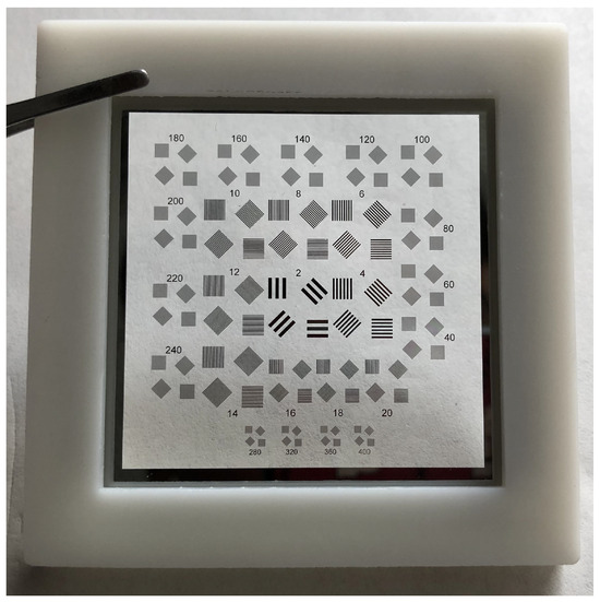
Figure 9.
Resolution Test Target. The group number represents the number of line pairs per millimeter.
Because of this magnification relationship, the spatial frequency on the resolution test board is of the spatial frequency on the image plane. Therefore, the actual spatial frequency corresponding to the lines of group 8 is about 165 lp/mm, of group 6 is about 124 lp/mm, and of group 4 corresponds to 83 lp/mm.
The results of the target test are shown in Figure 10. Figure 10a shows the coded low-resolution intermediate image captured by the WFC system and downsampled, the corresponding sensor-limited spatial resolution of which is approximately 55.6 lp/mm. Finally, the coded intermediate images were reconstructed using the sampled PSF. Figure 10b shows the decoded image using the bicubic interpolation method, in which the lines of group 4 with a spatial resolution of 83/2 = 41.5 lp/mm can be clearly distinguished, while those of group 6 are almost indistinguishable. Figure 10c displays the super-resolution decoded image following the approach detailed in the literature [51], in which the lines of group 6 can be separated but remain blurred. Figure 10d displays the image obtained through super-resolution reconstruction using SRGAN, in which the lines of group 6 can be partially separated, indicating a noticeable super-resolution effect. Figure 10e displays the image obtained using SwinIR for super-resolution reconstruction, in which the lines of group 6 with a spatial resolution of 124 lp/mm are fully separable, demonstrating the most prominent super-resolution effect.
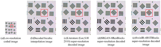
Figure 10.
Target image super-resolution reconstruction results. (a) The coded low-resolution image. (b) The super-resolution image decoded by bicubic interpolation method. (c) The super-resolution image decoded by the method detailed in [51]. (d) The super-resolution image reconstructed by SRGAN-8ResBlocks. (e) The super-resolution image reconstructed by SwinIR-6RSTBlocks. The red frame is the horizontal line in the group 6, corresponding to the resolution of 62 lp/mm (low-resoluition image) and 124 lp/mm (super-resolution image).
To quantify the performance of our super-resolution reconstruction, we plotted the intensity profiles along the blue dashed line in Figure 10d and the red dashed line in Figure 10e, as shown in Figure 11. Figure 11 shows the intensity distribution of resolution lines of the ideal resolution test target (grey line) and the SwinIR decoding (red line) and SRGAN decoding (blue line) result images. The corresponding full width at half maximum (FWHM) data and the average FWHM value are listed in Table 3. Through analysis of the image and corresponding FWHM data, we observe that SwinIR decoding achieves higher resolution, greater uniformity, and more effective reconstruction of image details compared to SRGAN. Overall, the intensity distribution of SwinIR’s lines aligns more closely with the ideal resolution lines. The experimental results show that the proposed method can achieve super-resolution from 55 lp/mm to 124 lp/mm, and the resolving ability is better than that of the original detector (111 lp/mm).
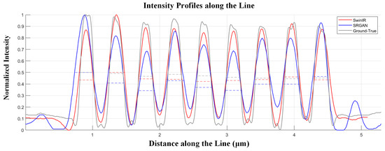
Figure 11.
The intensity distribution of resolution lines of the ideal resolution test target (grey line), SwinIR decoding (red line) and SRGAN decoding (blue line) result images. The dashed line is the corresponding full width at half maximum.
Table 3.
FWHM for corresponding lines (m).
We conducted experiments in outdoor scenes using the assembled camera (WFC) system and the experiment conditions are shown in Figure A4. The results are shown in Figure 12, Figure 13 and Figure 14. In each figure, (a) is the coded low-resolution image captured by the detector and downsampled, (b) is the decoded image using Wiener filtering, (c) is the decoded super-resolution image of the method in the literature [51], (d) is the super-resolution reconstructed image based on the SRGAN-8ResBlocks network structure, and (e) is the super-resolution reconstructed image based on the SwinIR-6RSTBlocks network structure. By judging the image quality by subjective feeling, it can be observed that the super-resolution reconstruction algorithms of the latter two networks are more advantageous in terms of image clarity. Among them, the super-resolution reconstruction algorithm based on the SwinIR-6RSTBlocks network provides richer detail reconstruction, better aligning with subjective visual effect, and exhibits superior performance in detail resolution ability and clarity.
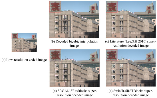
Figure 12.
Wavefront-coded super-resolution reconstruction results (Scene I).(a) The coded low-resolution image. (b) The super-resolution image decoded by bicubic interpolation method. (c) The super-resolution image decoded by the method detailed in [51]. (d) The super-resolution image reconstructed by SRGAN-8ResBlocks. (e) The super-resolution image reconstructed by SwinIR-6RSTBlocks.
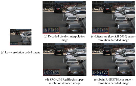
Figure 13.
Wavefront-coded super-resolution reconstruction results (Scene II). (a) The coded low-resolution image. (b) The super-resolution image decoded by bicubic interpolation method. (c) The super-resolution image decoded by the method detailed in [51]. (d) The super-resolution image reconstructed by SRGAN-8ResBlocks. (e) The super-resolution image reconstructed by SwinIR-6RSTBlocks.
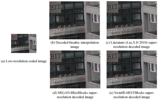
Figure 14.
Wavefront-coded super-resolution reconstruction results (Scene III). (a) The coded low-resolution image. (b) The super-resolution image decoded by bicubic interpolation method. (c) The super-resolution image decoded by the method detailed in [51]. (d) The super-resolution image reconstructed by SRGAN-8ResBlocks. (e) The super-resolution image reconstructed by SwinIR-6RSTBlocks.
The three images within the actual scene were objectively evaluated using the average gradient [52] evaluation criterion, and the results are shown in Table 4. Based on the average gradient values, it is apparent that the reconstruction method based on the SRGAN-8ResBlocks network can significantly enhance the contrast of the images, but the effect is limited and requires further enhancement in terms of sharpness. In Scene II, it has been observed that the reconstruction method based on the SwinIR-6RSTBlocks network can improve the average gradient value by 74.81%. The image gradient can be improved, resulting in higher contrast and clearer images after reconstruction. The improvement in image sharpness is more pronounced, and the reconstruction of image details is richer.
Table 4.
Comparison of the average gradients of super-resolution reconstruction images for different real-world scenes.
5. Conclusions
In this paper, we investigate a super-resolution reconstruction method in detector downsampling mode with improved frame rate based on wavefront coding technology. By utilizing a combination of deep learning networks to achieve super-resolution image reconstruction through the high-resolution PSF of the coding process, we investigate three representative deep learning network structures, and achieved training of the networks by modifying the depths of two of them. The simulation results show that the super-resolution algorithm based on deep learning network is superior to the traditional super-resolution decoding algorithm, and the network structure SwinIR based on Swin transformer obtained from the MAE loss training can produce more realistic super-resolution images. Finally, the combination of the proposed algorithm and a wavefront coding system has been demonstrated to improve the resolving ability of the system from 55.6 to 124 line pairs per millimeter during a resolution board test, while the average gradient of the image was enhanced by approximately 67% during a real-world scene experiment. To address the issues of low SSIM and extended training and running times of the model, we will implement a series of adjustments and optimizations in future research.
Author Contributions
X.L. and Y.W. conceived the idea and developed the strategy of the project. H.D. and Y.W. designed the theoretical wavefront coding system. H.Y. developed the network structure and designed the experiments. X.L. and H.Y. finished the original manuscript. H.Y., L.Z., D.C. and X.C. reviewed and edited the manuscript. All authors contributed to data analysis and paper writing. All authors have read and agreed to the published version of the manuscript.
Funding
This work was supported by the Zhejiang Provincial Natural Science Foundation of China under Grant No. LQ23F050014 and Zhejiang Provincial Department of Education Scientific Research Project under Grand No. Y202250682.
Data Availability Statement
The data of the experiments are not shared.
Acknowledgments
Thanks to the College of Computer Science and Artificial Intelligence of Wenzhou University and Beijing Key Laboratory for Precision Optoelectronic Measurement Instrument and Technology of Beijing Institute of technology for use of their equipment.
Conflicts of Interest
The authors declare no conflicts of interest.
Appendix A. Traditional Optical Imaging System and WFC System
Figure A1 shows diagrams of a traditional optical imaging system (without phase mask) and a WFC system (with phase mask) and the corresponding MTFs [42]. Figure A1a shows an initial structure of a lens that contains five single lenses, two doublet lenses, and a protective glass, with characterization of the aperture F Number is 0.95. Building on the traditional imaging system, we increased the aperture of the optical system while maintaining the same focal length. Initial optimization was achieved by adjusting the lens spacing, modifying the surface curvature, and reordering the doublet lenses. To correct for edge field aberrations, the seventh surface of the system (marked in orange) was modified to be an even-order aspherical surface. The surface mathematical equation is as follows:
where C represents the vertex curvature of the aspherical surface, k is the conic constant, r is the normalized radial distance, and are the coefficients for each even-order term. The final designed system with the enlarging aperture F/# = 0.75 is shown as Figure A1b.
In the MTF, the cut-off frequency corresponding to the diffraction limit reflects the system’s maximum resolving capability. However, as illustrated in Figure A1c, the bandwidth of the MTF in traditional optical systems is relatively high at the optimal focus position, containing ample image information. However, when the focus deviates from this optimal position, the MTF bandwidth decreases rapidly, often resulting in an excessively low cutoff frequency. In such off-focus positions, the MTF fails to meet the requirements for super-resolution, falling far short of the diffraction limit. In contrast, the MTF curve of our designed WFC system, shown in Figure A1d, exhibits distinct characteristics. As the spatial frequency increases, the MTF curve gradually approaches zero while remaining parallel without any zeros. Additionally, when the object distance deviates from the best focus position, the amplitude of the MTF curve does not change significantly. This entire process can be regarded as a coding process, enabling us to obtain encoded images with consistent blurring within the depth of focus range, providing the necessary information for super-resolution reconstruction. Therefore, although the MTF bandwidth is not particularly high, it contains sufficient information for super-resolution reconstruction. The intermediate coded images obtained through the WFC process can be decoded to produce much clearer super-resolution images.
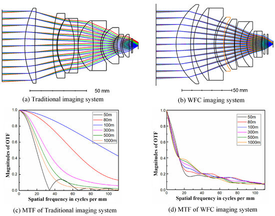
Figure A1.
Traditional optical imaging system (without phase mask) and WFC system (with phase mask). (a,c) are the diagram of traditional imaging system and the corresponding MTF curves with different object distance from 50 to 1000 m. (b,d) are the diagram of WFC imaging system and the corresponding MTF curves with different object distance from 50 to 1000 m. The orange surface is the phase mask. The color lines in the diagram represent the optical path with different field of view.
Appendix B. The Main Preset Parameters for the WFC Imaging System
The parameters of the designed WFC imaging system are detailed in the table below. This optical imaging system features a F/# of 0.75, an effective aperture diameter of 77.33 mm, and a focal length of 58 mm. The system boasts a field of view of and operates within the visible wavelength range. Additionally, it has a pixel size of 4.5 m and a depth of field extending from 50 to 1000 m.
Table A1.
Main preset parameters of WFC imaging system.
Table A1.
Main preset parameters of WFC imaging system.
| Parameters | Value |
|---|---|
| Focal length | 58 mm |
| F Number | 0.75 |
| Aperture | 77.33 mm |
| Field of view | |
| Wavelength range | visible |
| Pixel size | 4.5 m |
| Depth of field | 50 m∼1000 m |
| Sensor-limited resolution | Approximately 111 LP/mm |
Appendix C. Experiment Platform for Super-Resolution Reconstruction
The experimental setup, as shown in Figure A3, consists of a resolution target, a collimator, our designed wavefront coding optical system, a CCD camera, and a computer. The resolution target and collimator serve as the imaging objects. Our designed optical system functions like a camera, capturing intermediate coded images. These coded images are then processed by a computer to obtain clear decoded images.
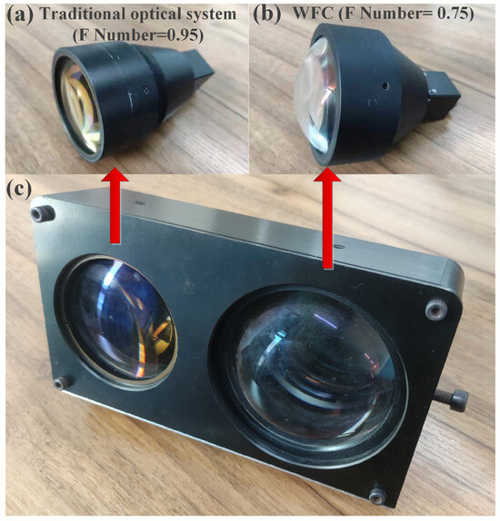
Figure A2.
Prototypes of designed system. (a) Traditional optical lens with F Number of 0.95. (b) WFC lens with F Number of 0.75. (c) Combination of the two systems.
Figure A2.
Prototypes of designed system. (a) Traditional optical lens with F Number of 0.95. (b) WFC lens with F Number of 0.75. (c) Combination of the two systems.


Figure A3.
The resolution target experimental setup.
Figure A3.
The resolution target experimental setup.
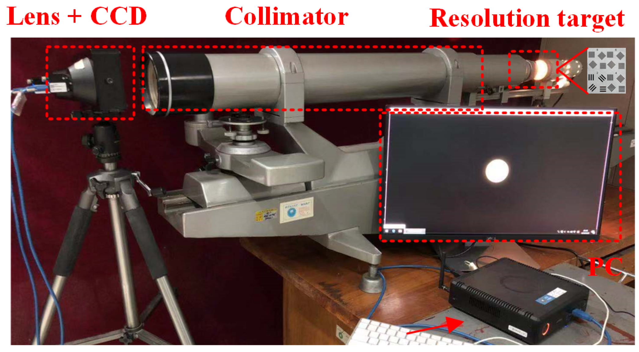
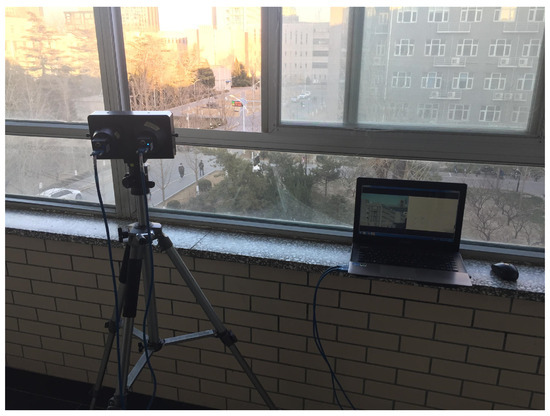
Figure A4.
The outdoor experimental setup.
Figure A4.
The outdoor experimental setup.

In the outdoor experiment, the WFC imaging system functioned as a camera to capture outdoor scenes at a distance of 100 m. Subsequently, these intermediate images were processed using deep learning networks for super-resolution reconstruction.
References
- Sheinin, M.; O’Toole, M.; Narasimhan, S.G. Deconvolving Diffraction for Fast Imaging of Sparse Scenes. In Proceedings of the 2021 IEEE International Conference on Computational Photography (ICCP), Haifa, Israel, 23–25 May 2021; pp. 1–10. [Google Scholar]
- Robinson, A.W.; Moshtaghpour, A.; Wells, J.; Nicholls, D.; Chi, M.; MacLaren, I.; Kirkland, A.I.; Browning, N.D. Simultaneous high-speed and low-dose 4-D stem using compressive sensing techniques. arXiv 2023, arXiv:2309.14055. [Google Scholar]
- Zhao, X.Y.; Li, L.J.; Cao, L.; Sun, M.J. Bionic Birdlike Imaging Using a Multi-Hyperuniform LED Array. Sensors 2021, 21, 4084. [Google Scholar] [CrossRef] [PubMed]
- Huijben, I.A.; Veeling, B.S.; Janse, K.; Mischi, M.; van Sloun, R.J. Learning sub-sampling and signal recovery with applications in ultrasound imaging. IEEE Trans. Med Imaging 2020, 39, 3955–3966. [Google Scholar] [CrossRef] [PubMed]
- Iqbal, O.; Muro, V.I.T.; Katoch, S.; Spanias, A.; Jayasuriya, S. Adaptive subsampling for ROI-based visual tracking: Algorithms and FPGA implementation. IEEE Access 2022, 10, 90507–90522. [Google Scholar] [CrossRef]
- Ortega, E.; Nicholls, D.; Browning, N.D.; de Jonge, N. High temporal-resolution scanning transmission electron microscopy using sparse-serpentine scan pathways. Sci. Rep. 2021, 11, 22722. [Google Scholar] [CrossRef] [PubMed]
- Wu, H.; Wang, R.; Zhao, G.; Xiao, H.; Liang, J.; Wang, D.; Tian, X.; Cheng, L.; Zhang, X. Deep-learning denoising computational ghost imaging. Opt. Lasers Eng. 2020, 134, 106183. [Google Scholar] [CrossRef]
- Wang, P.; Liang, J.; Wang, L.V. Single-shot ultrafast imaging attaining 70 trillion frames per second. Nat. Commun. 2020, 11, 2091. [Google Scholar] [CrossRef]
- Chai, L.; Gharbi, M.; Shechtman, E.; Isola, P.; Zhang, R. Any-resolution training for high-resolution image synthesis. In Proceedings of the European Conference on Computer Vision, Tel Aviv, Israel, 23–27 October 2022; Springer: Berlin/Heidelberg, Germany, 2022; pp. 170–188. [Google Scholar]
- Möller, B.; Pirklbauer, J.; Klingner, M.; Kasten, P.; Etzkorn, M.; Seifert, T.J.; Schlickum, U.; Fingscheidt, T. A Super-Resolution Training Paradigm Based on Low-Resolution Data Only To Surpass the Technical Limits of STEM and STM Microscopy. In Proceedings of the IEEE/CVF Conference on Computer Vision and Pattern Recognition, Vancouver, BC, Canada, 17–24 June 2023; pp. 4262–4271. [Google Scholar]
- Wei, C.; Ren, S.; Guo, K.; Hu, H.; Liang, J. High-resolution Swin transformer for automatic medical image segmentation. Sensors 2023, 23, 3420. [Google Scholar] [CrossRef]
- Tang, M.; Han, Y.; Jia, D.; Yang, Q.; Cheng, J.X. Far-field super-resolution chemical microscopy. Light. Sci. Appl. 2023, 12, 137. [Google Scholar] [CrossRef]
- Fu, S.; Shi, W.; Luo, T.; He, Y.; Zhou, L.; Yang, J.; Yang, Z.; Liu, J.; Liu, X.; Guo, Z.; et al. Field-dependent deep learning enables high-throughput whole-cell 3D super-resolution imaging. Nat. Methods 2023, 20, 459–468. [Google Scholar] [CrossRef]
- Qiao, C.; Li, D.; Liu, Y.; Zhang, S.; Liu, K.; Liu, C.; Guo, Y.; Jiang, T.; Fang, C.; Li, N.; et al. Rationalized deep learning super-resolution microscopy for sustained live imaging of rapid subcellular processes. Nat. Biotechnol. 2023, 41, 367–377. [Google Scholar] [CrossRef] [PubMed]
- Qian, J.; Cao, Y.; Bi, Y.; Wu, H.; Liu, Y.; Chen, Q.; Zuo, C. Structured illumination microscopy based on principal component analysis. eLight 2023, 3, 4. [Google Scholar] [CrossRef]
- Gallegos-Cerda, S.D.; Hernández-Varela, J.D.; Chanona-Pérez, J.J.; Arredondo Tamayo, B.; Méndez Méndez, J.V. Super-Resolution Microscopy and Their Applications in Food Materials: Beyond the Resolution Limits of Fluorescence Microscopy. Food Bioprocess Technol. 2023, 16, 268–288. [Google Scholar] [CrossRef]
- Li, W.; He, P.; Lei, D.; Fan, Y.; Du, Y.; Gao, B.; Chu, Z.; Li, L.; Liu, K.; An, C.; et al. Super-resolution multicolor fluorescence microscopy enabled by an apochromatic super-oscillatory lens with extended depth-of-focus. Nat. Commun. 2023, 14, 5107. [Google Scholar] [CrossRef] [PubMed]
- Upreti, N.; Jin, G.; Rich, J.; Zhong, R.; Mai, J.; Zhao, C.; Huang, T.J. Advances in Microsphere-based Super-resolution Imaging. IEEE Rev. Biomed. Eng. 2024. online ahead of print. [Google Scholar] [CrossRef] [PubMed]
- Zhu, X.; Sahoo, S.K.; Adamo, G.; Tobing, L.Y.; Zhang, D.H.; Dang, C. Non-Invasive Super-Resolution Imaging Through Scattering Media Using Object Fluctuation. Laser Photonics Rev. 2024, 18, 2300712. [Google Scholar] [CrossRef]
- Ben-loghfyry, A.; Hakim, A. Total variable-order variation as a regularizer applied on multi-frame image super-resolution. Vis. Comput. 2024, 40, 2949–2959. [Google Scholar] [CrossRef]
- Jin, S.; Liu, M.; Guo, Y.; Yao, C.; Obaidat, M.S. Multi-frame correlated representation network for video super-resolution. In Proceedings of the 2023 International Conference on Computer, Information and Telecommunication Systems (CITS), Genoa, Italy, 10–12 July 2023; pp. 1–7. [Google Scholar]
- Paredes, A.L.; Conde, M.H.; Ibrahim, T.; Pham, A.N.; Kagawa, K. Spatio-temporal Super-resolution for CS-based ToF 3D Imaging. In Proceedings of the 2023 31st European Signal Processing Conference (EUSIPCO), Helsinki, Fnland, 4–8 September 2023; pp. 461–465. [Google Scholar]
- Dai, M.; Xu, H.; Meng, Z.; Yang, G. Research on super-resolution image reconstruction technology. In AOPC 2023: Optical Sensing, Imaging, and Display Technology and Applications; and Biomedical Optics; SPIE: Beijing, China, 2023; Volume 12963, pp. 193–205. [Google Scholar]
- Yin, J.; Xu, S.H.; Du, Y.B.; Jia, R.S. Super resolution reconstruction of CT images based on multi-scale attention mechanism. Multimed. Tools Appl. 2023, 82, 22651–22667. [Google Scholar] [CrossRef]
- Wang, S.; Tian, A.; Liu, B.; Wang, H.; Zhu, X.; Zhu, Y.; Wang, K.; Ren, K.; Zhang, Y. Design of a three-channel pixelated phase mask and single-frame phase extraction technique. Opt. Lasers Eng. 2024, 177, 108127. [Google Scholar] [CrossRef]
- Rothlübbers, S.; Strohm, H.; Eickel, K.; Jenne, J.; Kuhlen, V.; Sinden, D.; Günther, M. Improving image quality of single plane wave ultrasound via deep learning based channel compounding. In Proceedings of the 2020 IEEE International Ultrasonics Symposium (IUS), Las Vegas, NV, USA, 7–11 September 2020; pp. 1–4. [Google Scholar]
- Chen, R.; Tang, X.; Zhao, Y.; Shen, Z.; Zhang, M.; Shen, Y.; Li, T.; Chung, C.H.Y.; Zhang, L.; Wang, J.; et al. Single-frame deep-learning super-resolution microscopy for intracellular dynamics imaging. Nat. Commun. 2023, 14, 2854. [Google Scholar] [CrossRef]
- Zhang, J.; Shao, M.; Yu, L.; Li, Y. Image super-resolution reconstruction based on sparse representation and deep learning. Signal Process. Image Commun. 2020, 87, 115925. [Google Scholar] [CrossRef]
- Cao, X.; Yao, J.; Xu, Z.; Meng, D. Hyperspectral image classification with convolutional neural network and active learning. IEEE Trans. Geosci. Remote Sens. 2020, 58, 4604–4616. [Google Scholar] [CrossRef]
- Jiang, Y.; Li, C. Convolutional neural networks for image-based high-throughput plant phenotyping: A review. Plant Phenomics 2020, 2020, 4152816. [Google Scholar] [CrossRef] [PubMed]
- Dhillon, A.; Verma, G.K. Convolutional neural network: A review of models, methodologies and applications to object detection. Prog. Artif. Intell. 2020, 9, 85–112. [Google Scholar] [CrossRef]
- Jiang, X.; Wu, Y. Remote sensing object detection based on convolution and Swin transformer. IEEE Access 2023, 11, 38643–38656. [Google Scholar] [CrossRef]
- Hatamizadeh, A.; Nath, V.; Tang, Y.; Yang, D.; Roth, H.R.; Xu, D. Swin unetr: Swin transformers for semantic segmentation of brain tumors in mri images. In Proceedings of the International MICCAI Brainlesion Workshop, Virtual Event, 27 September 2021; Springer: Berlin/Heidelberg, Germany, 2021; pp. 272–284. [Google Scholar]
- He, X.; Zhou, Y.; Zhao, J.; Zhang, D.; Yao, R.; Xue, Y. Swin transformer embedding UNet for remote sensing image semantic segmentation. IEEE Trans. Geosci. Remote Sens. 2022, 60, 1–15. [Google Scholar] [CrossRef]
- Li, B.; Li, X.; Lu, Y.; Liu, S.; Feng, R.; Chen, Z. Hst: Hierarchical swin transformer for compressed image super-resolution. In Proceedings of the European Conference on Computer Vision, Tel Aviv, Israel, 23–27 October 2022; Springer: Berlin/Heidelberg, Germany, 2022; pp. 651–668. [Google Scholar]
- Dai, Q.; Cheng, X.; Zhang, L. Image denoising using channel attention residual enhanced Swin Transformer. Multimed. Tools Appl. 2024, 83, 19041–19059. [Google Scholar] [CrossRef]
- Ma, Y.; Lei, T.; Wang, S.; Yang, Z.; Li, L.; Qu, W.; Li, F. A Super-Resolution Reconstruction Method for Infrared Polarization Images with Sparse Representation of Over-Complete Basis Sets. Appl. Sci. 2024, 14, 825. [Google Scholar] [CrossRef]
- Kong, L.; Dong, J.; Ge, J.; Li, M.; Pan, J. Efficient frequency domain-based transformers for high-quality image deblurring. In Proceedings of the IEEE/CVF Conference on Computer Vision and Pattern Recognition, Vancouver, BC, Canada, 17–24 June 2023; pp. 5886–5895. [Google Scholar]
- Wang, Z.; Bovik, A.C. Mean squared error: Love it or leave it? A new look at signal fidelity measures. IEEE Signal Process. Mag. 2009, 26, 98–117. [Google Scholar] [CrossRef]
- Rad, M.S.; Bozorgtabar, B.; Marti, U.V.; Basler, M.; Ekenel, H.K.; Thiran, J.P. Srobb: Targeted perceptual loss for single image super-resolution. In Proceedings of the IEEE/CVF International Conference on Computer Vision, Seoul, Republic of Korea, 27 October–2 November 2019; pp. 2710–2719. [Google Scholar]
- Brassington, G. Mean absolute error and root mean square error: Which is the better metric for assessing model performance? In Proceedings of the EGU General Assembly Conference Abstracts, Vienna, Austria, 23–28 April 2017; p. 3574. [Google Scholar]
- Dong, L.; Du, H.; Liu, M.; Zhao, Y.; Li, X.; Feng, S.; Liu, X.; Hui, M.; Kong, L.; Hao, Q. Extended-depth-of-field object detection with wavefront coding imaging system. Pattern Recognit. Lett. 2019, 125, 597–603. [Google Scholar] [CrossRef]
- Kocsis, P.; Shevkunov, I.; Katkovnik, V.; Rekola, H.; Egiazarian, K. Single-shot pixel super-resolution phase imaging by wavefront separation approach. Opt. Express 2021, 29, 43662–43678. [Google Scholar] [CrossRef]
- Zhang, Q.; Bao, M.; Sun, L.; Liu, Y.; Zheng, J. Wavefront coding image reconstruction via physical prior and frequency attention. Opt. Express 2023, 31, 32875–32886. [Google Scholar] [CrossRef] [PubMed]
- Kanoun, B.; Ferraioli, G.; Pascazio, V. Assessment of GPU-Based Enhanced Wiener Filter on Very High Resolution Images. In Proceedings of the 2020 Mediterranean and Middle-East Geoscience and Remote Sensing Symposium (M2GARSS), Tunis, Tunisia, 9–11 March 2020; pp. 65–68. [Google Scholar]
- Lien, C.Y.; Tang, C.H.; Chen, P.Y.; Kuo, Y.T.; Deng, Y.L. A low-cost VLSI architecture of the bilateral filter for real-time image denoising. IEEE Access 2020, 8, 64278–64283. [Google Scholar] [CrossRef]
- Agarap, A.F. Deep learning using rectified linear units (relu). arXiv 2018, arXiv:1803.08375. [Google Scholar]
- Ledig, C.; Theis, L.; Huszár, F.; Caballero, J.; Cunningham, A.; Acosta, A.; Aitken, A.; Tejani, A.; Totz, J.; Wang, Z.; et al. Photo-realistic single image super-resolution using a generative adversarial network. In Proceedings of the IEEE Conference on Computer Vision and Pattern Recognition, Honolulu, HI, USA, 21–26 July 2017; pp. 4681–4690. [Google Scholar]
- Agustsson, E.; Timofte, R. Ntire 2017 challenge on single image super-resolution: Dataset and study. In Proceedings of the IEEE Conference on Computer Vision and Pattern Recognition Workshops, Honolulu, HI, USA, 21–26 July 2017; pp. 126–135. [Google Scholar]
- Bevilacqua, M.; Roumy, A.; Guillemot, C.; Alberi-Morel, M.L. Low-complexity single-image super-resolution based on nonnegative neighbor embedding. In Proceedings of the British Machine Vision Conference, Surrey, UK, 3–7 September 2012; BMVA Press: Durham, UK, 2012. [Google Scholar]
- Lee, S.H.; Park, N.C.; Park, K.S.; Park, Y.P. Upscaling image resolution of compact imaging systems using wavefront coding and a property of the point-spread function. JOSA A 2010, 27, 2304–2312. [Google Scholar] [CrossRef]
- Pan, B.; Lu, Z.; Xie, H. Mean intensity gradient: An effective global parameter for quality assessment of the speckle patterns used in digital image correlation. Opt. Lasers Eng. 2010, 48, 469–477. [Google Scholar] [CrossRef]


Disclaimer/Publisher’s Note: The statements, opinions and data contained in all publications are solely those of the individual author(s) and contributor(s) and not of MDPI and/or the editor(s). MDPI and/or the editor(s) disclaim responsibility for any injury to people or property resulting from any ideas, methods, instructions or products referred to in the content. |
© 2024 by the authors. Licensee MDPI, Basel, Switzerland. This article is an open access article distributed under the terms and conditions of the Creative Commons Attribution (CC BY) license (https://creativecommons.org/licenses/by/4.0/).