Abstract
In multivariate and multistep time series prediction research, we often face the problems of insufficient spatial feature extraction and insufficient time-dependent mining of historical series data, which also brings great challenges to multivariate time series analysis and prediction. Inspired by the attention mechanism and residual module, this study proposes a multivariate time series prediction method based on a convolutional-residual gated recurrent hybrid model (CNN-DA-RGRU) with a two-layer attention mechanism to solve the multivariate time series prediction problem in these two stages. Specifically, the convolution module of the proposed model is used to extract the relational features among the sequences, and the two-layer attention mechanism can pay more attention to the relevant variables and give them higher weights to eliminate the irrelevant features, while the residual gated loop module is used to extract the time-varying features of the sequences, in which the residual block is used to achieve the direct connectivity to enhance the expressive power of the model, to solve the gradient explosion and vanishing scenarios, and to facilitate gradient propagation. Experiments were conducted on two public datasets using the proposed model to determine the model hyperparameters, and ablation experiments were conducted to verify the effectiveness of the model; by comparing it with several models, the proposed model was found to achieve good results in multivariate time series-forecasting tasks.
1. Introduction
Time series data are numerical values used in complex networked systems to describe objects that vary over time [1,2,3]. The matrix is used as the mathematical expression for the time series, with m representing the number of exogenous driving variables, and the meaning of k is the data length of the time series. A univariate time series occurs when m = 1, while a multi-variate time series occurs when m is greater than 1 [4].
In various industries, including finance, electric power, tourism, and meteorology, extensive time series datasets are prevalent [5,6,7]. With these large-scale datasets, one can use historical observations to predict future data points, thus providing technical assistance for industry advancement.
In practice, for different time series forecasting tasks, the length and accuracy requirements of the time series forecasting data that people want to obtain are different. According to the different lengths of forecast data, time series forecasting tasks can be divided into single-step forecasting tasks and multi-step forecasting tasks. A forecasting task that obtains the data of a certain future time length by analyzing historical data is called single-step forecasting, while a forecasting task that obtains data of multiple future time lengths by processing and analyzing historical time series data is called multi-step forecasting [8,9,10]. Due to the accumulation of individual errors in multi-step prediction, the data length of multi-step prediction is usually longer than that of single-step prediction, but the prediction accuracy and model prediction performance will be poorer.
Since the time series forecasting task was proposed, researchers have made a lot of efforts in mining the features of historical series data and improving the forecasting accuracy of models. For simple univariate linear forecasting tasks, traditional time series analysis and forecasting methods such as AR (autoregressive), MA (moving average), ARMA (autoregressive moving average), and ARIMA (autoregressive integral moving average) have been proposed for forecasting [11,12,13,14]. These classical statistical time series analysis models can achieve good results in univariate linear time series forecasting tasks and have been improved and developed over the three to four decades following their introduction for a wide range of applications.
With the development of science and technology, the accuracy of univariate time series prediction can no longer meet the needs of research, and the time series data generated in practical applications are not univariate, so the prediction of multivariate time series data as well as the exploration of the relationship between variables has gradually become a research hotspot. In the early 1980s, with the introduction of the concept of artificial intelligence, many researchers began to explore a new method of time series forecasting—machine learning—and they used the classical machine learning methods and models, such as SVM (support vector machines), RF (random forests), and BP (back propagation), in the task of time series forecasting [15,16,17]. This machine learning approach tends to achieve better results when forecasting multivariate nonlinear time series data with smaller sample sizes than traditional time series analysis methods.
Since the 21st century, thanks to the development of the high-tech industry, people’s lives have generated massive time series data, and human society has entered the era of big data. These massive time series data often have the characteristics of high dimensionality and nonlinearity, and the prediction accuracy can no longer meet the expected prediction accuracy requirements when using previous machine learning methods or statistical methods to predict scenario tasks. Facing this challenge, researchers have further proposed deep learning methods such as RNN (recurrent neural network), LSTM (long short-term memory neural network), and GRU (gated recurrent unit neural network) to cope with the task of predicting and analyzing the massive multivariate time series in the era of big data and have achieved great success. However, the multivariate time series prediction task still faces many challenges at this stage, the most important of which are the insufficient feature extraction capability and insufficient time-dependent extraction of mainstream prediction networks.
Therefore, this paper proposes a multivariate time series forecasting method based on a convolution-residual gated recurrent hybrid model with a two-layer attention mechanism, which focuses on extracting the characteristic relationships and temporal dependencies among the series in multivariate time series data.
The main contributions of this work are as follows:
- 1.
- Introducing a two-layer attention mechanism to learn the correlation between features and the temporal relationship within the feature sequence, assigning higher weights to features with high correlation, eliminating the interference of irrelevant features, and improving the feature and dependency extraction capability of the model;
- 2.
- Introducing residual blocks and residual connections to deepen the depth of the network, realizing direct connections to strengthen the model expression capability, resolving the cases of gradient explosion and disappearance, and facilitating the propagation of gradients in the network;
- 3.
- Combined with CNN, the spatial relationship features of variables are extracted, which improves the problem of insufficient spatial feature extraction in multivariate time series prediction.
The experimental results show that the proposed model has good predictive ability and performance on two public datasets: financial and environmental.
The structure of the rest of this paper is as follows: The second section introduces the related work involved in this paper, the third section introduces the structure of the CNN-DA-RGRU model, the fourth section discusses the experimental results, and the last part is the summary of the research.
2. Related Works
The introduction of the AR model in 1927 opened the door to modern time series analysis. In the following years, models such as MA, ARMA and ARIMA were successively proposed [13,14]. For simple univariate linear time series forecasting problems, these classical statistical models can do the job perfectly and show good results. However, when faced with slightly more complex multivariate nonlinear time series forecasting problems, these methods are somewhat out of their depth. In the early 1980s, with the progress of science and technology and the concept of artificial intelligence, scholars successively proposed some classical machine learning methods, such as SVM, BP, RF, and so on [16,17,18,19,20]. These methods have been developed and applied to multivariate nonlinear time series forecasting tasks. These machine learning methods can effectively focus on different sequence values of multiple variables in a multivariate series. At the same time, however, they have the fatal flaw that they tend to ignore the time dependence of the data in the series, leading to simple regression fits to the data. Therefore, when one wants to predict multivariate nonlinear time series with a large amount of data, the prediction accuracy of these machine learning methods is mostly unsatisfactory.
Since the 1990s, deep learning methods have been used in time series forecasting. The proposal of RNN also improved the accuracy of complex multivariate nonlinear time series forecasting tasks on a higher level [21]. Deep learning methods are gradually being studied and applied to the field of prediction.
In 1997 and 2014, two variants of RNN, i.e., LSTM and GRU, were proposed, respectively [22,23]. Compared with traditional RNN models, LSTM and GRU can selectively filter information due to their unique gating structure and also avoid the problems of gradient vanishing and gradient explosion, which are prone to affecting the prediction accuracy of traditional RNN models. Ma et al. used LSTM and SAE as a prediction model for multivariate traffic speed prediction, and the results showed that the prediction performance of LSTM is better than SAE [24]. For the task of multi-variable solar photovoltaic time series prediction, Zameer et al. [25] proposed two kinds of improved models based on BILSTM and GRU. Compared with some classical machine learning algorithms, these two methods are more robust and have higher prediction accuracy for problems.
However, most of the proposed LSTM or GRU models face the dilemma of poor time-dependent extraction of sequence features, leading to insufficient prediction accuracy. In fact, when predicting multivariate nonlinear time series, the prediction results were found not only related to the data of the most recent historical moments before the prediction, but the distant historical data also had an impact on the prediction results [26]. In order to solve the problem of insufficient sequential time-dependent extraction, attention mechanisms were introduced into the model to enhance the prediction performance [27].
A novel two-stage attention-based recurrent neural network (DA-RNN) for multivariate time series prediction was proposed by Qin et al. They argued that the single-layer attention mechanism is unsuitable for multivariate time series prediction due to its susceptibility to disturbances, and experiments were carried out on several publicly available datasets to verify the superiority of the proposed model [28]. Based on the study of Qin et al., Cheng et al. proposed the DA-BiLSTM model due to multivariate prediction and achieved better results on three public datasets [29]. However, the above methods only focus on the temporal relationship within the data series, and they ignore the variable relationship between the series, that is, the spatial relationship between the series [30].
To solve this problem, most researchers use CNN and LSTM networks to extract the temporal and spatial relationships of time series at the same time. For multivariate time series prediction in the field of financial economy, Widiputra et al. proposed a multivariate CNN-LSTM and conducted related experiments, and the experimental results showed that the model achieved a small error in the task of financial economy [31]. Dogani et al. constructed a CNN-GRU model with an attention mechanism to predict loads in cloud computing and found that the model performed well at this task [32]. Gao et al. also used CNN-GRU to predict wind speed on a multivariate wind speed dataset based on the spatial feature extraction of CNN and the time-dependent feature of GRU extraction and achieved good prediction results [33]. In order to better solve the problems of model non-convergence and low prediction accuracy, Patel proposed a hybrid model combining CNN and LSTM, which was applied to the prediction of multi-variable solar irradiance [34]. In addition, Hu, Asadi, Berlati, Yu, and other scholars have also contributed to the application of multivariate forecasting [35,36,37,38,39,40,41]. Their results further validate the effectiveness of deep learning models in multivariate time series prediction under a hybrid framework of RNN variants and CNN or attention mechanisms.
Therefore, in this paper, based on the basic architectures of convolution neural networks and gated recurrent unit neural networks, we constructed a hybrid CNN-DA-RGRU architecture, which can be used for multivariate time series prediction tasks, by adding a double-layer attention mechanism between the two basic architectures and increasing the residual blocks through residual connections.
3. CNN-DA-RGRU Model
3.1. Problems and Evaluation Indicator
In this study, we propose a suitable solution to the problem of insufficient spatial feature extraction and time-dependent extraction in multivariate time series prediction. Among them, the number of exogenous variables, the size of the sliding time window, and the prediction time step are common important parameters in multivariate time series analysis and prediction tasks. Generally speaking, the matrix in space is usually used to represent the multivariate time series whose length is k and the number of variables to be predicted is m (the number of exogenous variables is m – 1). The vector in space is usually used to represent the predicted target sequence, so the total length of the target sequence is k. At the same time, for the i-th sequence of exogenous variables, it is usually represented by the vector in the space, while for all sequences of exogenous variables at the j-th time, it can be represented by the vector in the space.
In this study, our purpose is to predict the time series value of one or more time steps based on the historical data of exogenous variable time series of sliding time window with size w and the target sequence data of corresponding historical moment, which can be described in mathematical language as follows:
where is the exogenous variable sequence data with history time window size w, is the T-step target sequence data predicted based on the sequence data of exogenous variables with the historical time window size w, and is the parameter that needs to be learned during the training process of the model in this paper. is the target mapping function that needs to be trained and learned by the model in this paper, which will perform nonlinear mapping operations on historical and predicted data in a vector space.
In this study, we used three common error functions as evaluation indicators of model performance, namely MAE (mean absolute error), MAPE (mean absolute percentage error), and RMSE (root mean square error). When the values of RMSE, MAE, and MAPE decrease, it means that the error between the predicted value and the true value is reduced, and the closer to 0, the better the prediction effect of the model is. When RMSE, MAE, and MAPE are iterated to the minimum value, the model effect is optimal at this moment. The mathematical definitions of these indicators are as follows:
3.2. Method Flow and Model Structure
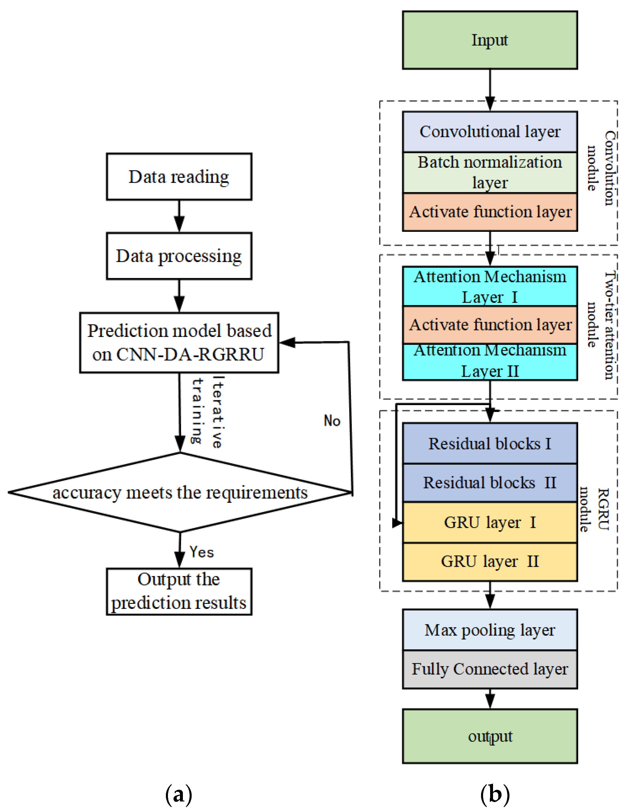
The flow of the multivariate time series prediction method based on the convolution-residual-gated cyclic hybrid model based on the two-layer attention mechanism is shown in the Figure 1a. This method consists of four steps:
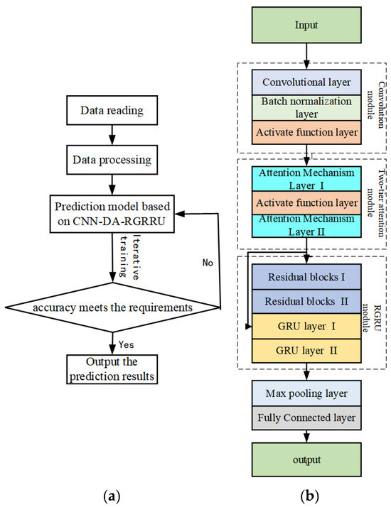
Figure 1.
(a) Algorithm flowchart; (b) CNN-DA-RGRU model structure.
- Step 1: Data reading and processing.
- Step 2: Model construction.
- Step 3: Model iterative training.
- Step 4: Output of the prediction results.
We propose a CNN-DA-RGRU model to alleviate the problem of insufficient feature and time-dependent extraction in prediction. The structure of the CNN-DA-RGRU model is shown in the Figure 1b, which includes an input layer, a convolution module, a two-layer attention mechanism module, a residual gating recurrent neural network module, a maximum pooling layer, and a fully connected layer. First, the processed data is taken as the initial input of this step and input into the input layer of the CNN-DA-RGRU model.
3.2.1. Convolution Module
The data are processed by the input layer into the convolution module and then processed by a layer of convolution network, a layer of batch normalization network, and a layer of activation function. In detail, the input data first enter a convolution layer for convolution processing, where the convolution layer is the value of the convolution kernel, and the value framed by the kernel is calculated by matrix multiplication, and the calculation formula is as follows:
where l represents the row of the time series image that is input to the convolution layer for the convolution operation, C represents the convolution operation, and represents the convolution kernel size. represents the result of the output of the i-th row vector and the j-th convolution kernel. is the output result of the convolution layer; through the processing of the convolution layer, the spatial features between variables of time series can be extracted initially, which is convenient for the in-depth extraction of internal time-dependent features of subsequent variable series. The preliminary extraction features are to cut the time series data according to a certain time interval, the data of each time period is a pixel value, and a plurality of time periods are combined into a one-dimensional image, and this time image is convoluted. The result of the convolution is input into a batch normalization layer, which is calculated as follows:
where is the normalized feature, is the original feature, is the smallest of all features, and is the maximum value of all features.
By batch normalization of the data, the data of different dimensions can be changed into data of the same dimension, and the variation range of all data can be limited to a region, making it easier for the model to learn effective feature representation. The output result of the batch normalization layer enters the activation function layer of the next layer, and the data enter the activation function layer and are processed by the sigmoid function to change the data change range, where the activation function layer function is the sigmoid function, and the calculation formula is as follows:
where compresses the values of the input activation function layer and converts the values into (0, 1) intervals.
Through the nonlinear transformation ability of the sigmoid function, the gradient transfer can be better processed, the gradient disappearing and explosion can be avoided, and the ability of the convolution module to learn data features can be used to realize the primary feature extraction of the experimental dataset and reduce the complexity of the prediction model.
3.2.2. Double-Layer Attention Mechanism Module
The spatial feature vector processed by the convolution module is input into the first attention layer, and then, through the activation function layer, the second attention layer is input. Generally speaking, the output of the convolution module is used as the input of the attention mechanism module and is input to the first attention layer, i.e., the additive attention layer; taking a single time window w as an example, the attention function of the first attention layer, i.e., the mapping from to , is expressed as . This additive attention layer is used to calculate the weights of each primary time feature, and the attention function of this layer is specifically expressed as Equation (8) to Equation (13).
where X is the input vector; , , and are parameter matrices that need to be learned. Q is the target value matrix, calculated by parameter matrix and input vector X, used to calculate the similarity with K. K is the keyword matrix, calculated by parameter matrix and input vector X, and used for similarity calculation with Q. V is the original matrix, calculated from the parameter matrix and the input vector X, used to calculate and obtain the weight. A is the matrix obtained after the similarity calculation of Q and K. is the matrix obtained by A through SoftMax function. T is the weight matrix.
The output of the additive attention layer is multiplied by the output of the convolution module to obtain the result , which is used as the input of the activation function layer of the next layer, and the dimensions of each variable are transformed into the same numerical interval through the nonlinear transformation of the activation function so as to improve the expressive ability of the model. The output of the activation function layer is input to the second attention layer, and the attention function is the mapping from to , which is denoted as . The formula for this layer’s attention function is same as Equation (8) to Equation (13).
The purpose of this module is to extract data features in depth and then multiply and add the attention weight and the output data of the convolution module one by one to output to the next module.
3.2.3. Residual Gated Recurrent Neural Network Module
The features vector obtained by the attention mechanism module is fed into the residual gated recurrent neural network module through two residual blocks on the one hand, and on the other hand, in order to speed up the convergence of the network and to reduce the gradient explosion and vanishing, a residual structure is introduced, including a branch, and the output of the branch is added to the backbone network through convolution and is fed into the two gated recurrent neural networks along with the outputs of the residual blocks of the backbone network. The data obtained through the double-layer attention mechanism module are taken as the initial input of this module, and the residual gated recurrent neural network module is input. The data first enter the first residual block, and the purpose of this is to realize a direct connection to strengthen the expression ability of the model and solve the gradient explosion and disappearance, and its calculation can be expressed as given:
where is the input; represents the output function of the first residual block.
The data processed by the first residual block are input into the second residual block, which boosts the propagation of the gradient in the network, accelerates the convergence speed of the network, increases the path of information flow to directly transmit the information of the previous layer to the later layer, and enables the network to learn more complex and deep feature representations to improve performance and strengthen the performance of the network; the formula of the second residual block is expressed as follows:
At the same time, the branch of the residual structure of the input data processed by the attention mechanism module is denoted as given below:
where is the convolution function on the branch.
The data processed by two residual blocks and residual structures are input into the first gated recurrent neural network layer, which is represented as , used to initially establish the time series relationship between the data and learn the trend of historical data for predicting future trends. The data are processed by the first gated recurrent neural network layer and input to the second gated recurrent neural network layer, which is used to extract relevant features from the time series data for prediction.
The gated recurrent neural network layer takes as input. Each gated recurrent neural network layer contains two gates: The update gate and reset gate as well as a hidden state are used to control information flow transmission and filtering so as to enhance the memory and expression ability of the model. At each time step, the input vector and the previous hidden state are linearly transformed and then input to the memory cells controlled by the two gates. Here, the calculation method for each gated recurrent neural network layer is as follows:
In the formula, is an update gate; is reset door; x is the input; is the hidden state, that is, the hidden layer output result. and are added to obtain , and is the weight matrix of the gated recurrent neural network layer.
3.2.4. Max Pooling Layer
The data vector processed by the residual gated recurrent neural network module is a two-dimensional vector, which is sequentially fed into the dimensional reduction layer of the maximum pooling layer and the fully connected layer, and the output of the fully connected layer is output as the model prediction result. When this vector is fed into the maximum pooling layer, the model downscales this two-dimensional vector using a pooling kernel, which is also called maximum pooling because it takes the maximum value of the current pooling kernel. After processing by the maximum pooling layer, the main features of the data are preserved to avoid the over-fitting of the model. The pooled parameters are calculated as follows:
In this equation, N represents the output size of the convolution layer, W stands for input size, F stands for convolution kernel size, P represents the filling value size, and S is a small step.
The formula for calculating the pooled kernel is similar to that for calculating the convolution layer, taking the mean of the sum of the values in the pooled kernel frame:
where represents the output result of the i-th row vector and the j-th pooled kernel, and w is the number of row vectors.
3.2.5. Fully Connected Layer
The output results of the pooling layer are input to the fully connected layer for learning higher-level features. The activation function is Relu and the calculation formula for this layer is as follows:
where the symbol @ represents linear operations at the fully connected layer, and is the input vector. is the weight vector of the three hidden layers; is the bias of the three hidden layers. is the result of the first hidden layer forward calculation, and the Relu function is calculated for the linear weighted summation of and plus . is the result of forward calculation of the second hidden layer, and the Relu function is calculated for the result of linear weighted summation of and plus . is the output of the fully connected layer and the result of the forward calculation of the third hidden layer. The Relu function is calculated for the linear weighted summation of and plus .
In this layer, the input vector is reconstructed, stretched into a one-dimensional shape, and matrix multiplication is performed on the input vector and the weight matrix. The result of matrix multiplication is combined with the input activation function of the bias vector for nonlinear transformation processing. Finally, the output of the fully connected layer is obtained as the prediction result of the model.
4. Experimental Design and Analysis
4.1. Experimental Setup
The experiment was conducted on an HP Shadow Wizard 9 consisting of Windows 11 operating system, Intel i5 core, 3.7 GHz CPU, 16 GB RAM, and Nvidia RTX 4060, using the programming language python and the deep learning framework Pytorch 1.13.1 and Tensorflow 2.13.1.
A total of two multivariate time series datasets were used in this experiment; the two public datasets were the SML2010 dataset [42] and the exchange rate dataset [43]. The SML2010 dataset selected indoor temperature as the target sequence of this time series prediction experiment, and the other 16 sequences were taken as exogenous variable sequences related to the experimental target sequence. The exchange rate dataset selects the Singapore exchange rate series as the target series of this time series prediction experiment, and the other seven sequences were selected as the exogenous sequences of the experiment target. Both datasets were divided into the training set, the validation set, and the test set in a ratio of 8:1:1. The exact size of the dataset is shown in Table 1. The parameters of CNN-DA-RGRU are shown in Table 2.

Table 1.
Dataset partitioning.
Table 2.
Parameters of proposed CNN-DA-RGRU.
SML2010 dataset: The dataset was collected from a house built specifically for the Solar Decathlon Competition. The dataset contains about 40 days of monitoring data with a granularity of 15 min. It mainly includes 21 types of time series data, such as indoor temperature, outdoor temperature and relative humidity, among which there are 4137 data in each category.
Exchange rate dataset: The exchange rate dataset contains a daily exchange rate summary of eight countries from 1990 to 2016 for 26 years, including Australia, the United Kingdom, Canada, Switzerland, China, Japan, New Zealand, and Singapore, with a time granularity of 1D, eight variable series, and 7589 pieces of data.
To verify the prediction performance of the model in this chapter, RMSE, MAE, MAPE were used as the evaluation metric, and the SML2010 dataset and the exchange rate dataset were used as the experimental datasets.
In the experiment, we set the size of the sliding time window and gradually increased it to perform the single-step prediction experiment so that the sliding time window was set to 5, 10, 15, 20, 25, 30 and 50.
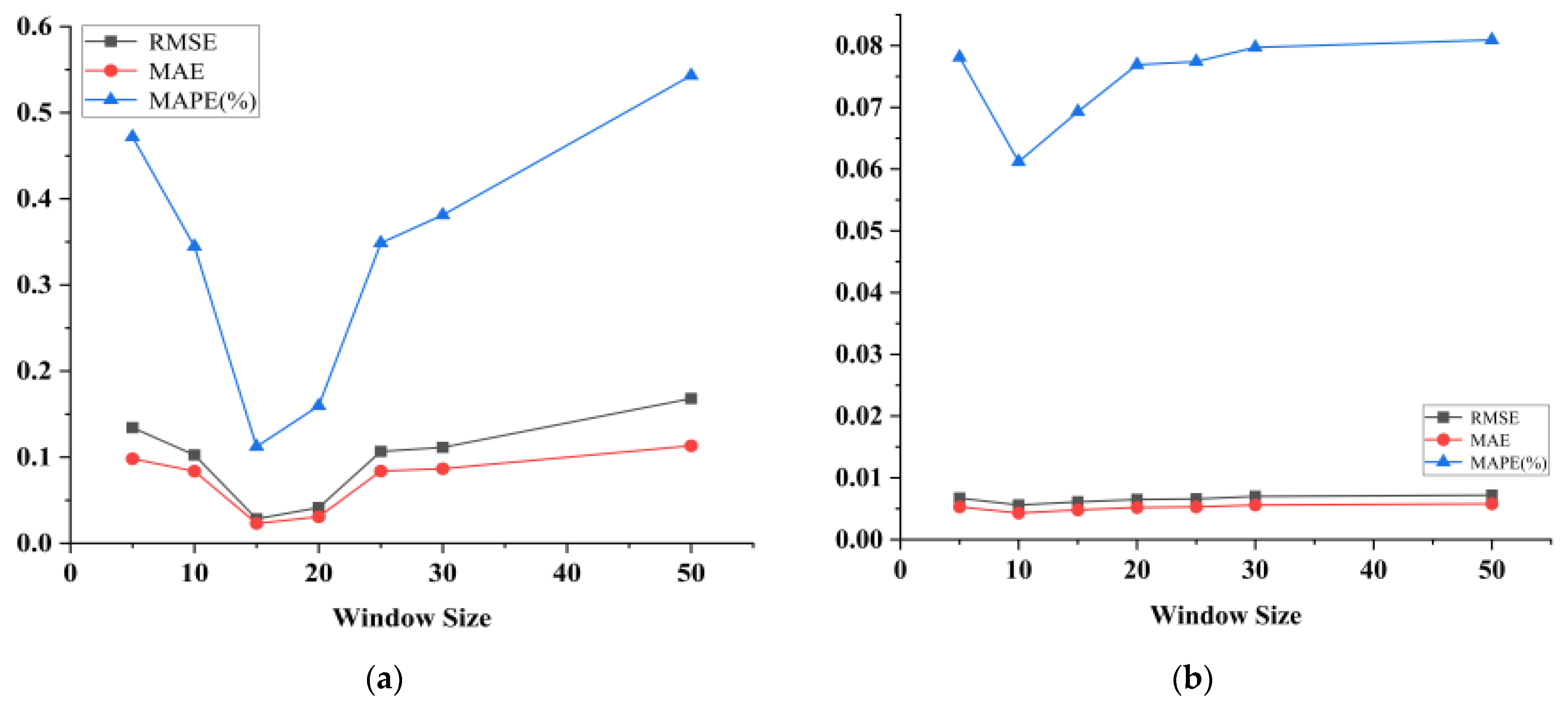
Figure 2 shows the relationship between the sliding window size set in the experiments for the two datasets and the results of the model evaluation metrics. As can be seen in Figure 2a, for the SML2010 dataset, the RMSE and MAE of the model range from 0 to 0.2, while the MAPE fluctuates from 0.1 to 0.5. When the sliding window size is set to 15, the RMSE, MAE, and MAPE reach the lowest values. This indicates that the prediction error of the model is minimized. From Figure 2b, it can be seen that for the exchange rate dataset, the RMSE and MAE of the model fluctuate between 0 and 0.01, while the MAPE fluctuates between 0.06 and 0.08. When the experiment gradually increases the sliding window size from 5, the RMSE, MAE, and MAPE decrease until the window size is equal to 10, when all three evaluation indexes reach the minimum value. When the window size is equal to 10, all three evaluation indicators reach the minimum value. It can be seen that when the sliding window size is set to 10, the model has the best prediction performance for the exchange rate dataset.
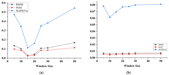
Figure 2.
Plot of time window results on the SML2010 dataset and exchange rate dataset, listed as (a) results on the SML2010 dataset; (b) results on the exchange rate dataset.
In addition to the variation of sliding time windows, choosing different convolution kernel sizes, different pooling kernel sizes, and different hidden layer unit sizes in the experiments can also lead to different prediction results. Therefore, in order to minimize the impact of parameter variations on the experimental results, we conducted parameter sensitivity experiments on the one-step prediction-based CNN-DA-RGRU model on two datasets to determine the convolution kernel size, the pooling kernel size, and the hidden layer unit size.
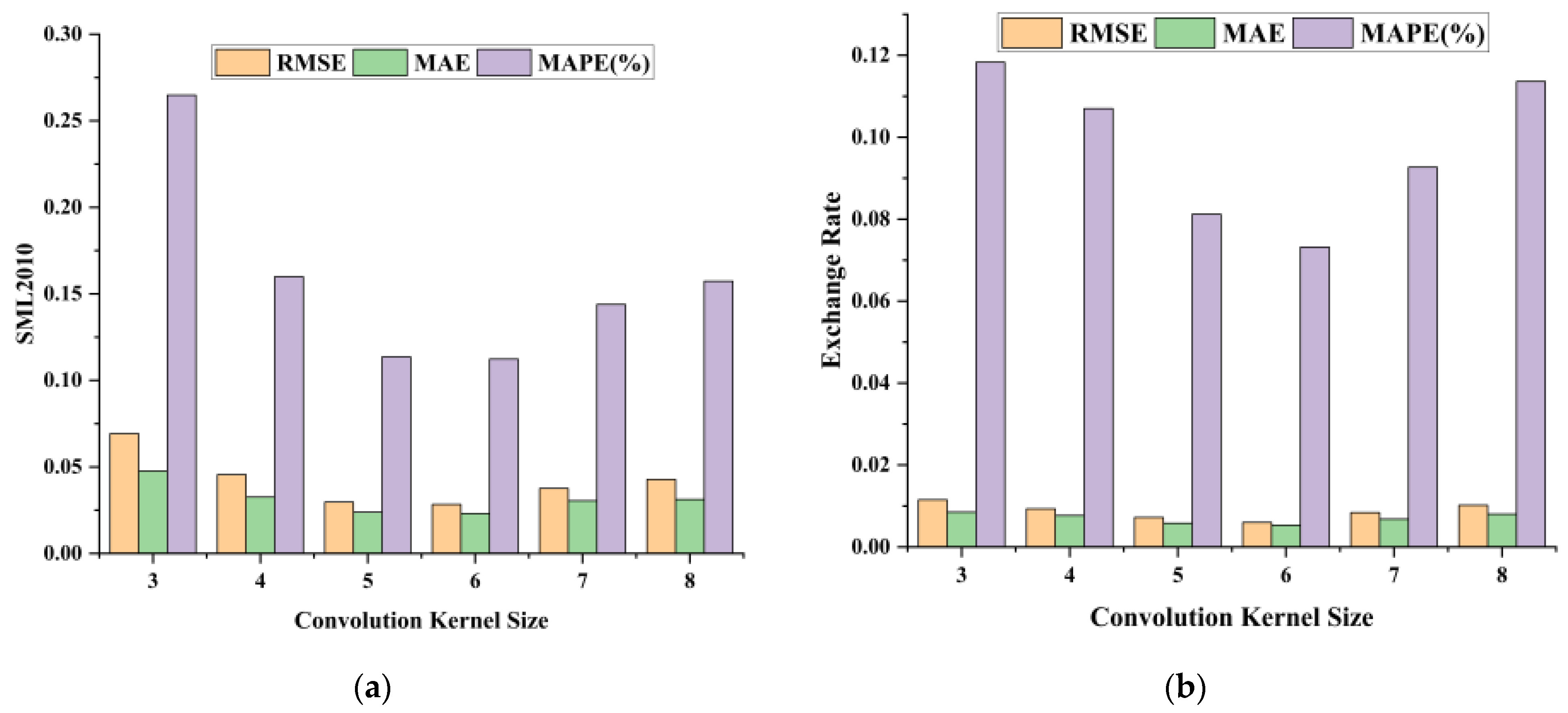
We first performed experiments on the sensitivity of the convolution kernel size. The other parameter settings were consistent with the results of the sliding time window experiments. In the experiments, the convolution kernel size was varied sequentially from 3 to 8 to observe the changes in RMSE, MAE, and MAPE. Figure 3 shows the relationship between the convolution kernel size and the three metrics on the two datasets. It can be seen that when the convolution kernel size is 6, the three indicators on both datasets reach the minimum value; i.e., the model has the strongest spatial feature extraction ability and the best prediction results.
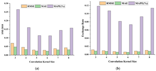
Figure 3.
Plot of convolution kernel size results on the SML2010 dataset and exchange rate dataset, listed as (a) results on the SML2010 dataset; (b) results on the exchange rate dataset.
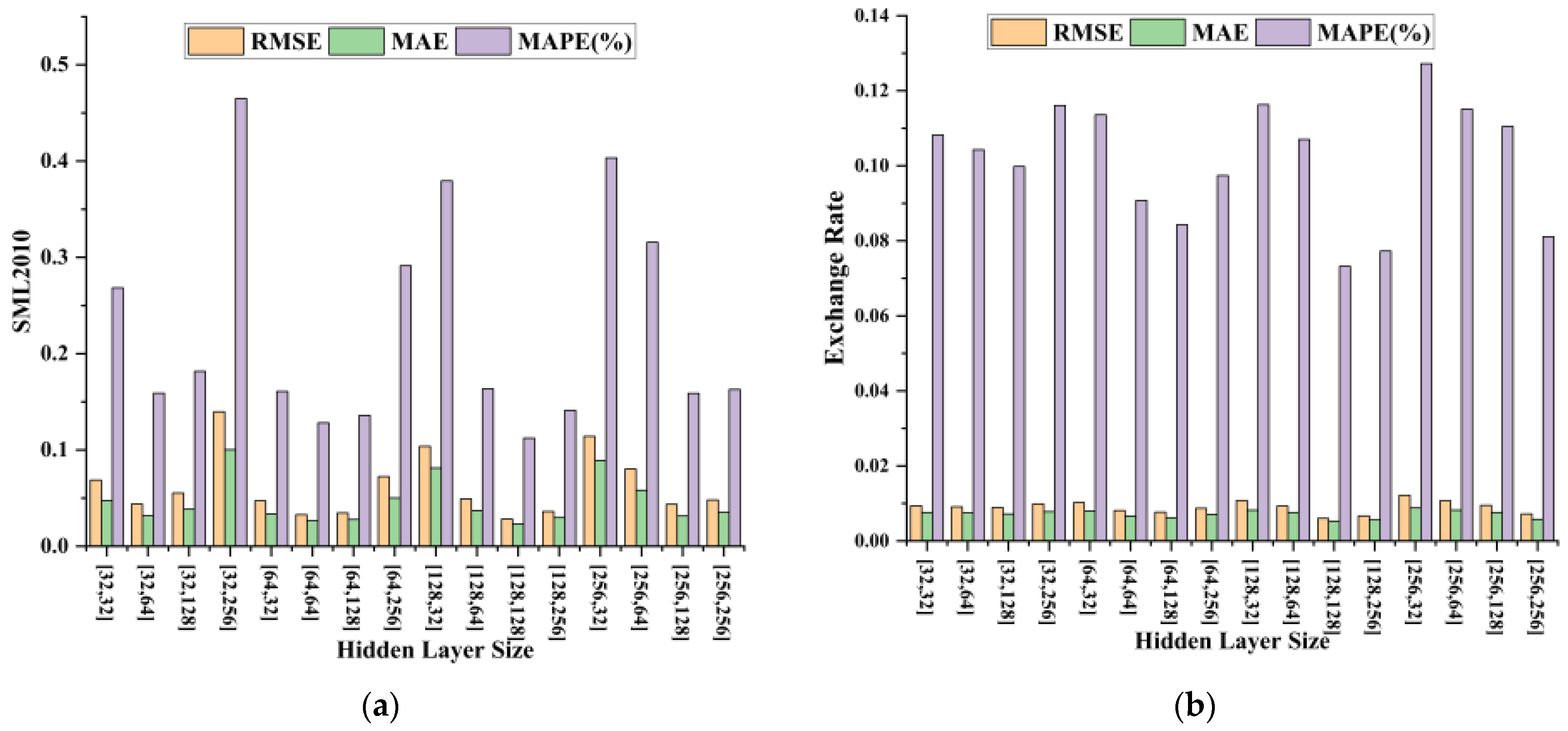
Based on our determination of the size of the convolution kernel and the size of the sliding time window, we then conducted sensitivity experiments on the size of the GRU hidden layer element, and the settings of other parameters in the experiment were consistent with the above experiments. In the experiment, we set up 16 combinations of two hidden layers with sizes 32, 64, 128, and 256 and observed the changes in three types of evaluation indicators. Figure 4 shows the relationship between the size of the hidden layer unit and the three indicators on two types of datasets. It can be seen that when the hidden layer unit size is [128, 128], the RMSE, MAE, and MAPE show the minimum values, which also indicates that the model has the best time-dependent extraction ability at this time.
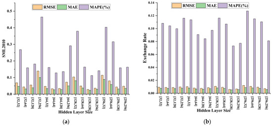
Figure 4.
This is a plot of hidden layer size results on the SML2010 dataset and exchange rate dataset, listed as (a) results on the SML2010 dataset; (b) results on the exchange rate dataset.
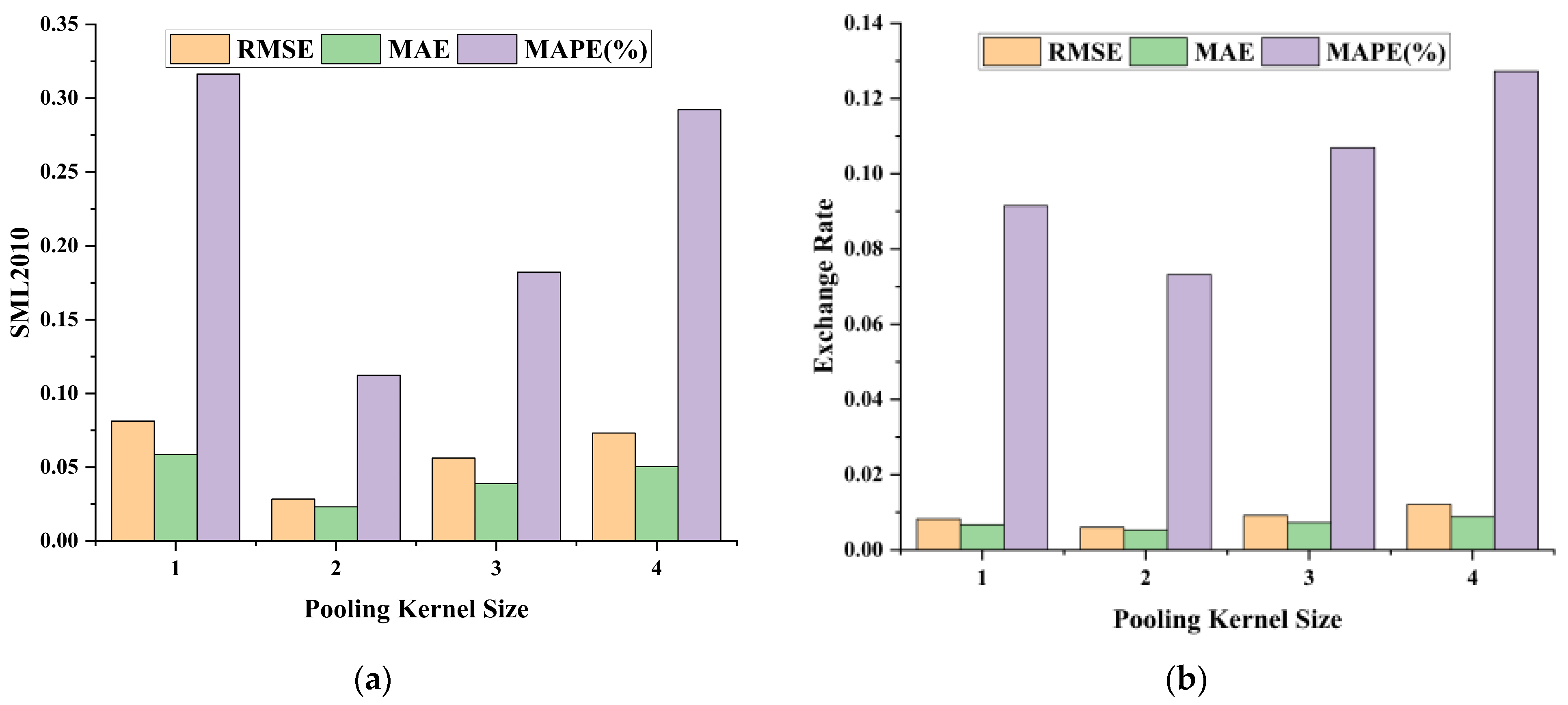
Finally, based on the determination of the size of the convolution kernel, the size of the sliding time window, and the size of the hidden layer unit, we carried out the sensitivity experiment of the pool kernel size, and the other parameters were set by the above experiment. The size of the pooled nucleus was selected as 1, 2, 3, and 4, respectively, and the changes of RMSE, MAE, and MAPE were observed. Figure 5 shows the relationship between the size of pooled cores and the three metrics on the two datasets. As can be seen from the figure, when the pooled kernel is 2, the three evaluation indicators all obtain the minimum value, which indicates that the model has the strongest ability to eliminate redundant features at this time.
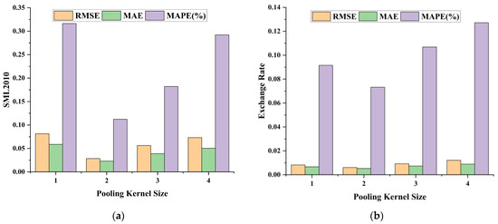
Figure 5.
Plot of pooling kernel size results on the SML2010 dataset and exchange rate dataset, listed as (a) results on the SML2010 dataset; (b) results on the exchange rate dataset.
4.2. Ablation Experiments
To verify the effectiveness of different modules, namely CNN, DA, and RGRU, we conducted ablation experiments on two datasets. The models containing different components are as follows:
With a single-layer attention module only: We replaced the two-layer attention module in the model with a single-layer attention module, and the model is labeled CNN-DA-RGRU1.
Without the two-layer attention module: We removed the two-layer attention module from the model and recorded the model as CNN-DA-RGRU2.
Without the convolution module: We removed the convolution module from the model and recorded the model as CNN-DA-RGRU3.
Without the residual structure module: We removed the residual module from the model and recorded the model as CNN-DA-RGRU4.
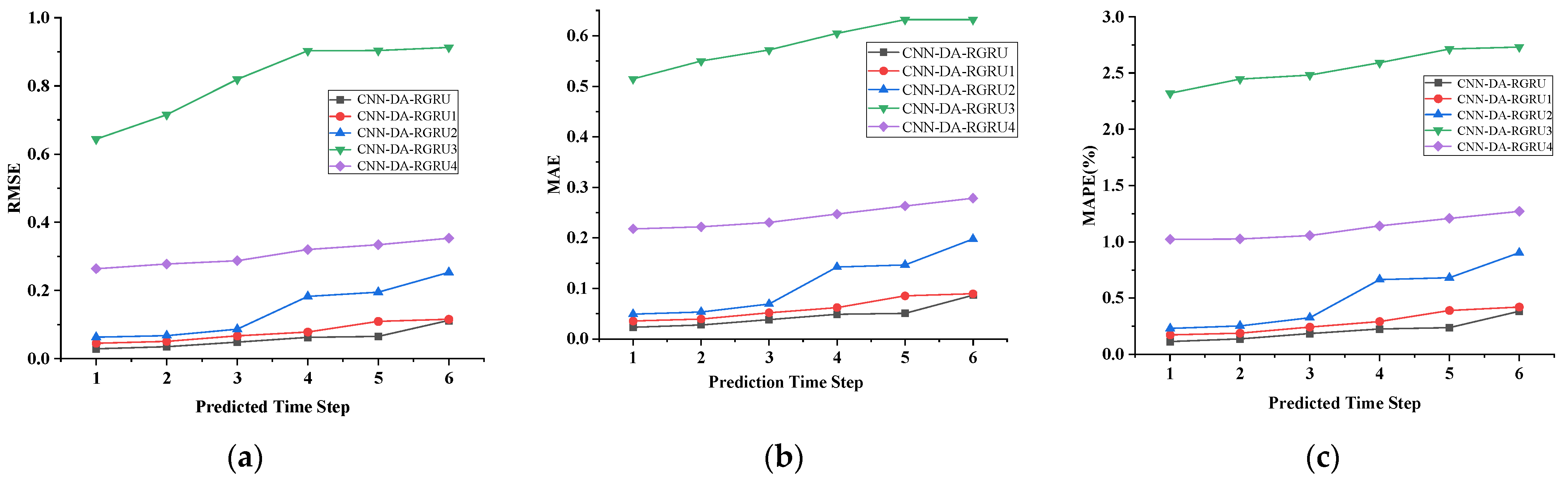
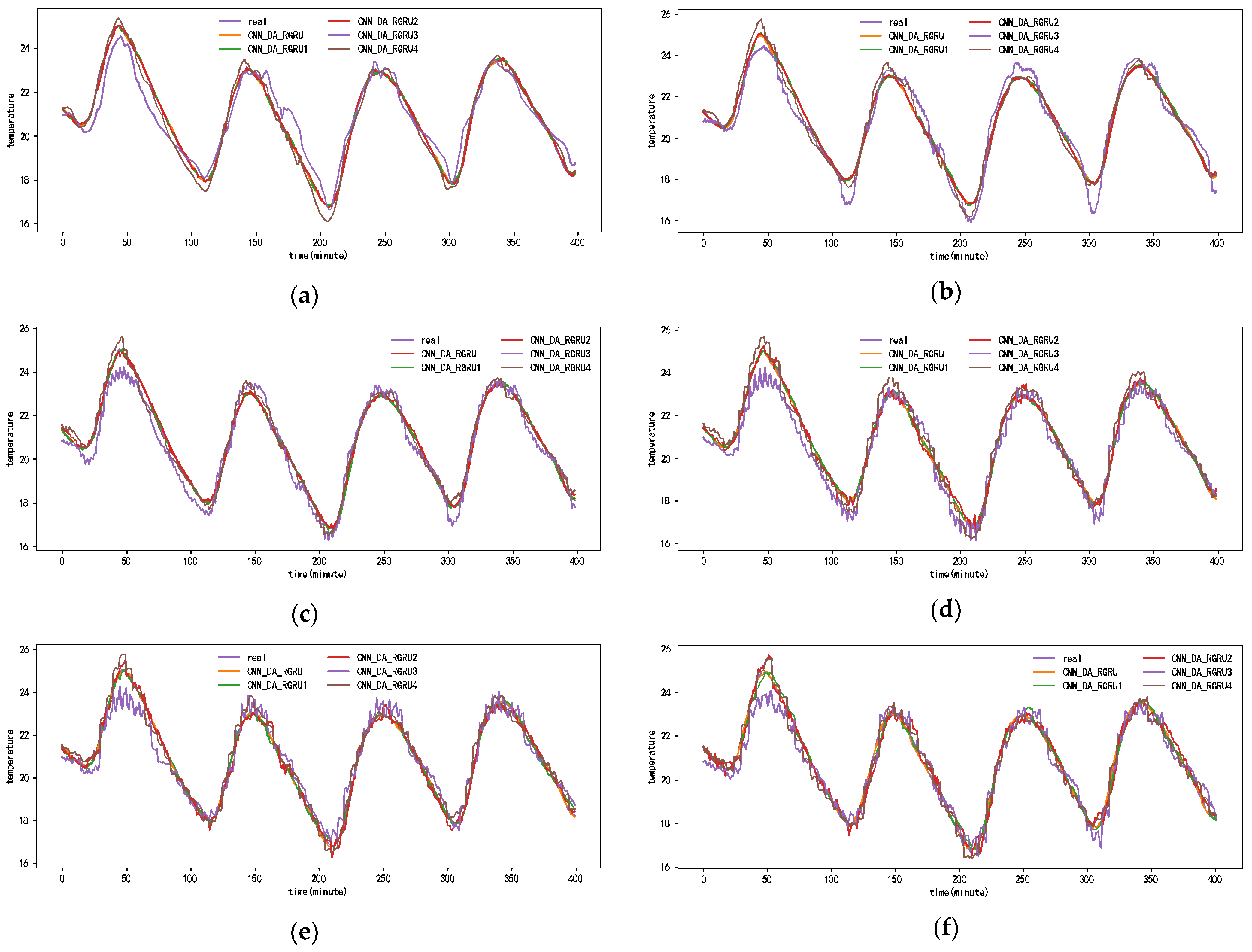
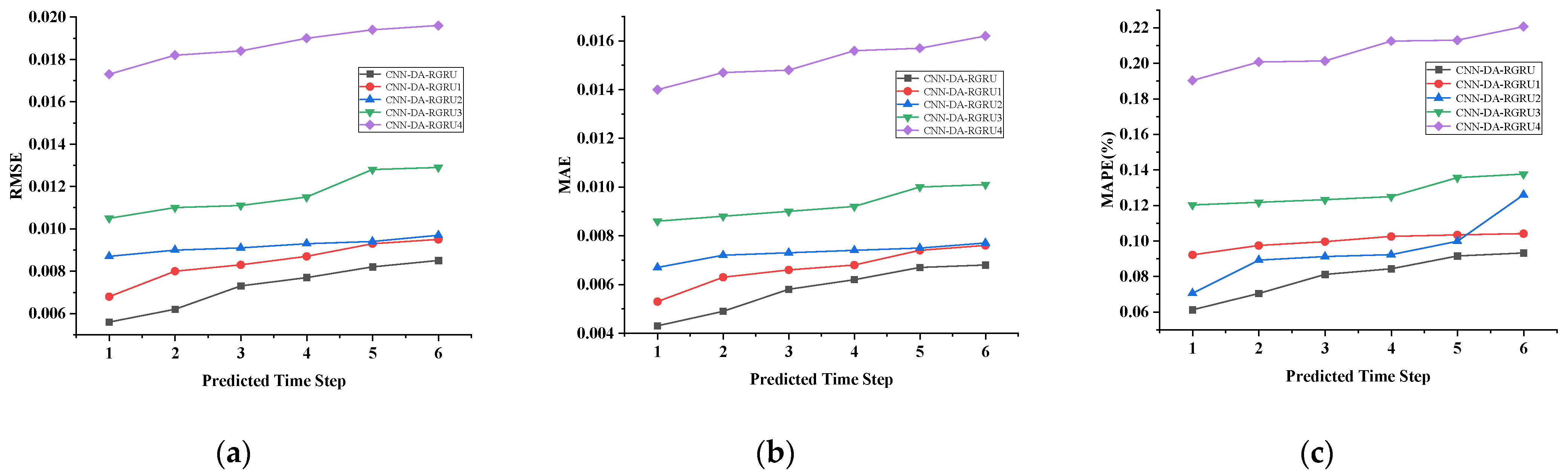
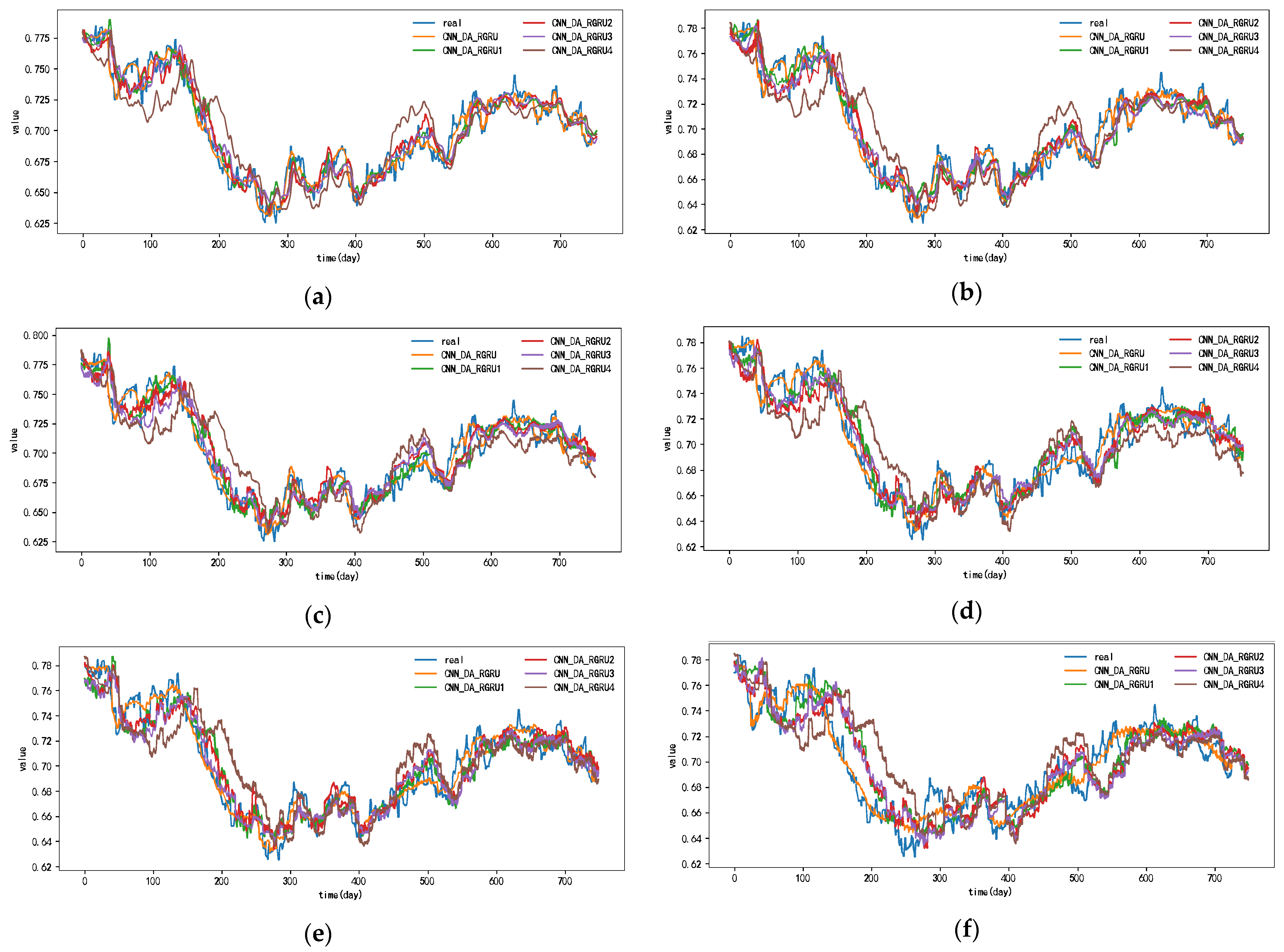
Figure 6, Figure 7, Figure 8 and Figure 9 show the metric results, actual values, and predictions of the CNN-DA-RGRU model and the ablation model on the SML2010 and exchange rate datasets. As can be seen from the figure, the introduction of the convolution module greatly improves the prediction results since it can extract the spatial relationship between sequences. The prediction results of the two-layer attention model are better than those of the single-layer attention model. Removing residual connections also reduces the prediction performance of the model. In the ablation experiments on the SML2010 dataset, the prediction performance of all the above structures, in descending order, is CNN-DA-RGRU > CNN-DA-RGRU1 > CNN-DA-RGRU2 > CNN-DA-RGRU4 > CNN-DA-RGRU3. This shows that in the ablation experiments on the SML2010 dataset, the removal of residual connections has the largest impact, followed by removing the convolution module, followed by reducing the number of layers of attention, and the smallest impact is the removal of the two-layer attention module. In the ablation experiments on the exchange rate dataset, the predictive performance of all the above structures, in descending order, is CNN-DA-RGRU > CNN-DA-RGRU1 > CNN-DA-RGRU2 > CNN-DA-RGRU3 > CNN-DA-RGRU4. This shows that removing residual joins has the greatest impact in the ablation experiments on the exchange rate dataset, followed by the removal of the convolution module, followed by the removal of the two-layer attention module, with the smallest impact being the reduction in the number of attention layers.
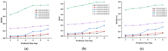
Figure 6.
Evaluation metrics results of ablation experiment on the SML2010 dataset, listed as (a) RMSE; (b) MAE; (c) MAPE.
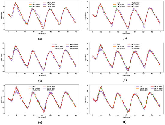
Figure 7.
Results of ablation experiment on the SML2010 dataset, listed as (a) 1-step results; (b) 2-step results; (c) 3-step results; (d) 4-step results; (e) 5-step results; (f) 6-step results.
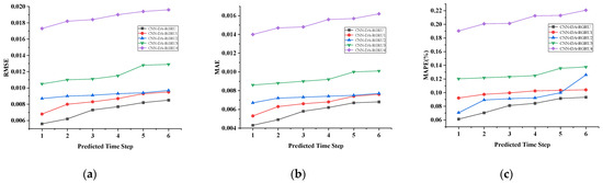
Figure 8.
Evaluation metrics results of ablation experiment on the exchange rate dataset, listed as (a) RMSE; (b) MAE; (c) MAPE.
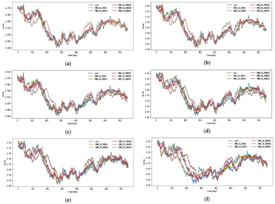
Figure 9.
Results of ablation experiment on the exchange rate dataset, listed as (a) 1-step results; (b) 2-step results; (c) 3-step results; (d) 4-step results; (e) 5-step results; (f) 6-step results.
4.3. Comparative Experiments
In this experiment, a total of 13 deep learning models in multivariate prediction problems were selected and compared with CNN-DA-RGRU on public datasets.
(1) GRU: Che et al. constructed a GRU model for a multivariable time series prediction and achieved good results [30];
(2) BIGRU: This is a bidirectional gated recurrent unit neural network based on GRU;
(3) GRU-Attention: Jung et al. proposed a predictive model combining GRU and attention mechanism for power prediction, and the results show that this model is superior to other models [45];
(4) BIGRU-Attention: Song et al. used the BIGRU-Attention model to forecast the multi-variable tropical cyclone track dataset, and the experimental results showed that the accuracy of this model was improved compared with the mainstream prediction models in tropical cyclone tracking and prediction tasks [46];
(5) CNN-GRU: Gao et al. proposed a CNN-GRU model for wind speed prediction on multivariate wind speed dataset and achieved good prediction effect [33];
(6) CNN-BIGRU: This is a hybrid architecture combining CNN and bidirectional gated recurrent neural network based on CNN-GRU;
(7) LSTM: Sorkun et al. proposed a multivariate LSTM prediction model using multivariate meteorological data to predict solar radiation and compared the results with previous studies, finding that the multivariate approach performed better than the previous univariate model [47];
(8) BILSTM: This is a bidirectional long short-term memory neural network model based on LSTM;
(9) LSTM-Attention: Ju and Liu proposed the LSTM-Attention model, and the experiments results show that the model has an excellent performance [48];
(10) BILSTM-Attention: Hao et al. proposed a prediction model of atmospheric temperature based on the BILSTM-Attention model, and the results show that the BILSTM-Attention prediction model can effectively improve the prediction accuracy [49];
(11) CNN-LSTM: Widiputra et al. proposed a hybrid architecture of multiple CNN-LSTM, which showed its superiority in multiple financial forecasting tasks [31];
(12) CNN-BILSTM: Kim et al. used CNN and BILSTM to construct a mixed model to study the system marginal price of Jeju Island in South Korea, and the research results show that the model has a good forecasting performance in this forecasting task [50];
(13) DSA-Conv-LSTM: Xiao et al. used the two-stage attention mechanism and Conv-LSTM to construct a hybrid architecture for multivariate time series prediction, and the results show that this model has advantages over other baseline models [30].
Table 3, Table 4 and Table 5 present MAE, MAPE, and RMSE evaluation indicators of each baseline model and the prediction results of the model on the SML2010 dataset. As can be seen from the table, the prediction results of single GRU, LSTM, BIGRU, and BILSTM are smaller than those of the corresponding models with the attention mechanism added, regardless of the single- or multi-step prediction. This is because after the attention mechanism is added, based on the attention mechanism, the model pays more attention to the properties of important features and pays more attention to the features that are important and related to the target sequence variables, thus improving the performance of multivariate prediction. In addition, we can also see from the table that since convolutional networks can effectively extract spatial features, that is, relational features between variables, the combined model combined with convolutional networks also performs better than the single model without convolutional networks. In this comparison experiment, in addition to the model proposed in this paper, the DSA-Conv-LSTM model has the best prediction effect because the DSA-Conv-LSTM model can effectively extract spatial relationships and important features by using the convolution layer and the two-stage attention mechanism layer. The ability of the two-stage attention mechanism to extract important features is stronger than that of the general attention mechanism.
Table 3.
The prediction results of RMSE evaluation metric of SML2010 dataset.
Table 4.
The prediction results of MAE evaluation metric of SML2010 dataset.
Table 5.
The prediction results of MAPE (%) evaluation metric of SML2010 dataset.
However, the DSA-Conv-LSTM model also has its shortcomings. We found that although the model works best in single-step prediction, the error increases greatly with the increase in step size, so the accuracy is not ideal in multi-step prediction. This is because in the process of calculating the model, the error of a large amount of information will accumulate, followed by the problem of gradient disappearance and explosion. In contrast, our proposed CNN-DA-RGRU model contains a residual structure that provides a direct connection across layers. The data processed by the convolutional module are added to the branch input of the next module, thus breaking the symmetry of the network, reducing the degradation of the network and solving the error accumulation problem mentioned earlier. Compared with the suboptimal DSA-Conv-LSTM model, in 2–6 prediction steps, the RMSE index of this model decreased by 0.0153, 0.0122, 0.0562, 0.0584, and 0.0491; the MAE index decreased by 0.0083, 0.0055, 0.0396, 0.0423, and 0.0167; and the MAPE error decreased by 0.0379%, 0.0031%, 0.2035%, 0.1776%, and 0.1191%, respectively. Also, observing the errors accumulated in the six-step prediction of this paper’s model and the suboptimal model, the errors accumulated in the six-step prediction of DSA-Conv-LSTM for RMSE are 0.0242, 0.009, 0.0609, 0.0106, and 0.0293; the errors accumulated in MAE are 0.0172, 0.0035, 0.0507, 0.0023, and 0.0122; the MAPE-accumulated errors are 0.0816%, 0.0174%, 0.2246%, 0.0265%, and 0.0772%, respectively. The CNN-DA-RGRU model predicted the RMSE metrics in these six steps with sequential cumulative errors of 0.0063, 0.0197, 0.0136, 0.0032, and 0.0466; the MAE metrics with sequential cumulative errors of 0.0047, 0.0071, 0.0063, 0.0023, and 0.0451; and the MAPE metrics with sequential cumulative errors of 0.0236%, 0.0260%, 0.0204%, 0.1657%, and 0.0017% respectively. It can be seen that in the accumulation of multi-step prediction errors, the error accumulation of CNN-DA-RGRU is mostly smaller than that of DSA-Conv-LSTM. This also shows the effectiveness of the residual connection structure.
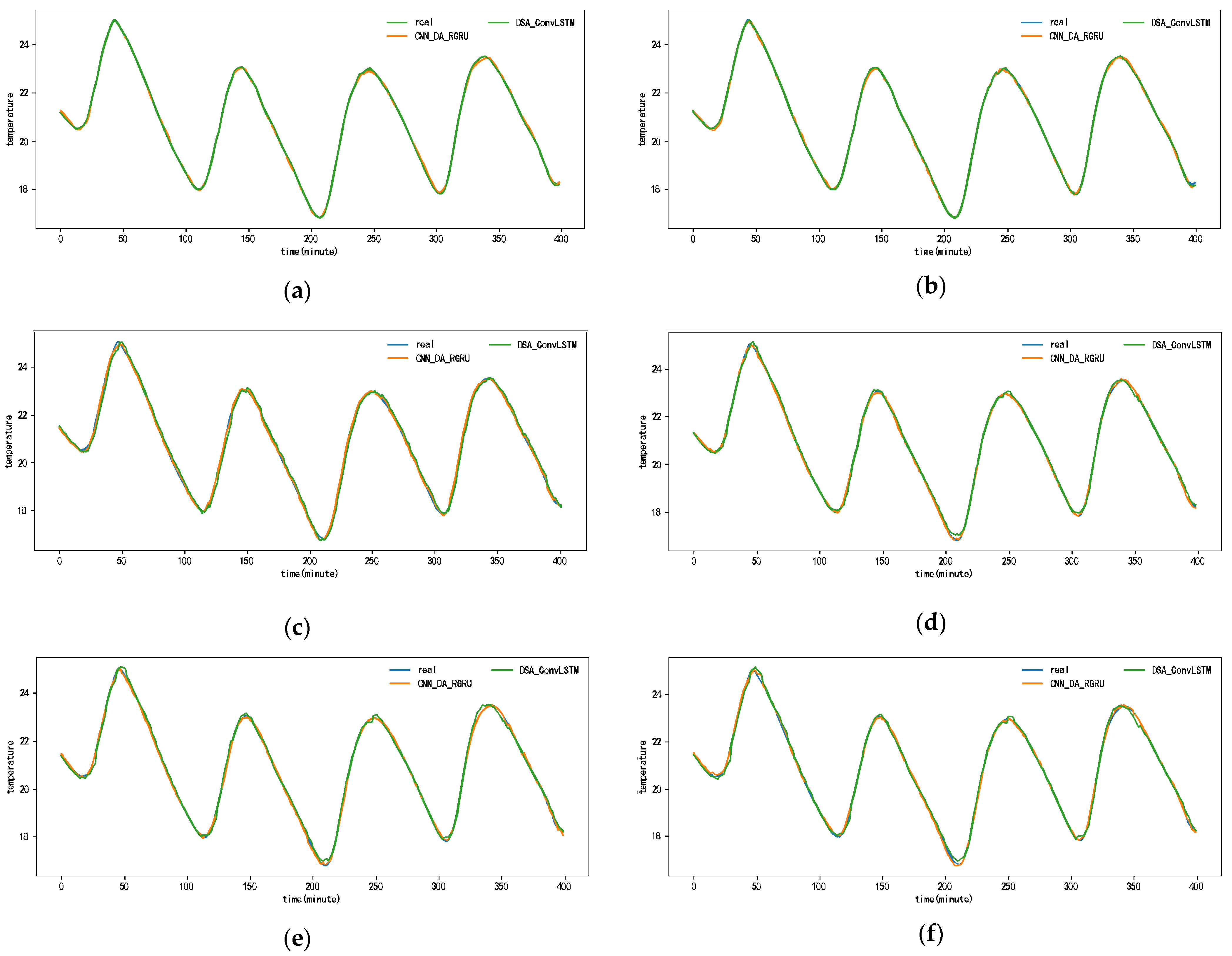
Figure 10 and Appendix A Figure A1, Figure A2, Figure A3, Figure A4, Figure A5 and Figure A6 show the predictions for each model on the SML2010 dataset. Since the prediction results of other comparison models except DSA-Conv-LSTM are significantly different from the CNN-DA-RGRU proposed in this paper, only the prediction results of DSA-Conv-LSTM and CNN-DA-RGRU are compared with the real values in Figure 10. It can be seen from the results in the figure that both the proposed model and the second-best model have better prediction performance for the SML2010 dataset, and the proposed model is superior. Therefore, from these chart data, we can see that the prediction performance of the CNN-DA-RGRU model proposed in this paper is slightly better than that of the DSA-Conv-LSTM model on the SML2010 dataset and also better than other baseline models.
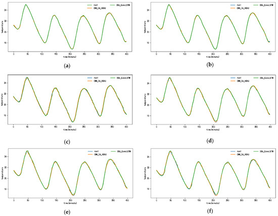
Figure 10.
The 1–6-step real values and forecast results of DSA-Conv-LSTM and proposed CNN-DA-RGRU on the SML2010 dataset, listed as (a) 1-step; (b) 2-step; (c) 3-step; (d) 4-step; (e) 5-step; (f) 6-step.
Table 6, Table 7 and Table 8 show the results of the MAE, MAPE, and RMSE evaluation metrics for the prediction effectiveness of each model on the exchange rate dataset. From the data in the table, it can be seen that the DSA-Conv-LSTM model has the best prediction effect except for the model proposed in this paper when the given prediction steps are 3–6 time steps. Compared with the second-ranked DSA-Conv-LSTM model, the RMSE metrics of this paper’s model are reduced by 0.0003, 0.0006, 0.0006 and 0.0007; the MAE metrics are reduced by 0.0007, 0.0007, 0.0005, and 0.0008; and the MAPE error was reduced by 0.003%, 0.0078%, 0.0081%, and 0.0137%. In the six-step prediction, DSA-Conv-LSTM increased the RMSE errors by 0.0003, 0.0017, 0.0007, 0.0005, and 0.0007, respectively; MAE by 0.0004, 0.0013, 0.0002, and 0.0004; and the cumulative MAPE errors by 0.00065%, 0.0137%, 0.008%, 0.0075%, and 0.0073%, respectively. The CNN-DA-RGRU model predicted 0.0002, 0.0011, 0.0004, 0.0005, and 0.0003 successive increases in the RMSE metrics and 0.0002, 0.0003, 0.0004, 0.0005, and 0.0001 successive increases in the MAE metrics in the six steps, and the MAPE indicator successively increased the error by 0.0047%, 0.0032%, 0.0032%, 0.0072%, and 0.0017%, respectively. It can be seen that in the multi-step prediction error accumulation, the error accumulation of CNN-DA-RGRU is smaller than that of DSA-Conv-LSTM. Secondly, the GRU-Attention model, CNN-GRU model, LSTM-Attention model, BILSTM-Attention model, and CNN-BILSTM model perform better in single-step pre-prediction because these model components contain attention or convolutional layers. They can effectively extract spatio-temporal features and give more weights to important features. In addition to the model proposed in this paper, the DSA-Conv-LSTM model still has the best prediction performance on this dataset because the DSA-Conv-LSTM model can extract spatio-temporal feature relationships and focus on important features. In single-step prediction and multi-step prediction, the CNN-DA-RGRU model outperforms the above models in general.
Table 6.
The prediction results of RMSE evaluation metric of the exchange dataset.
Table 7.
The prediction results of MAE evaluation metric of the exchange dataset.
Table 8.
The prediction results of MAPE (%) evaluation metric of the exchange dataset.
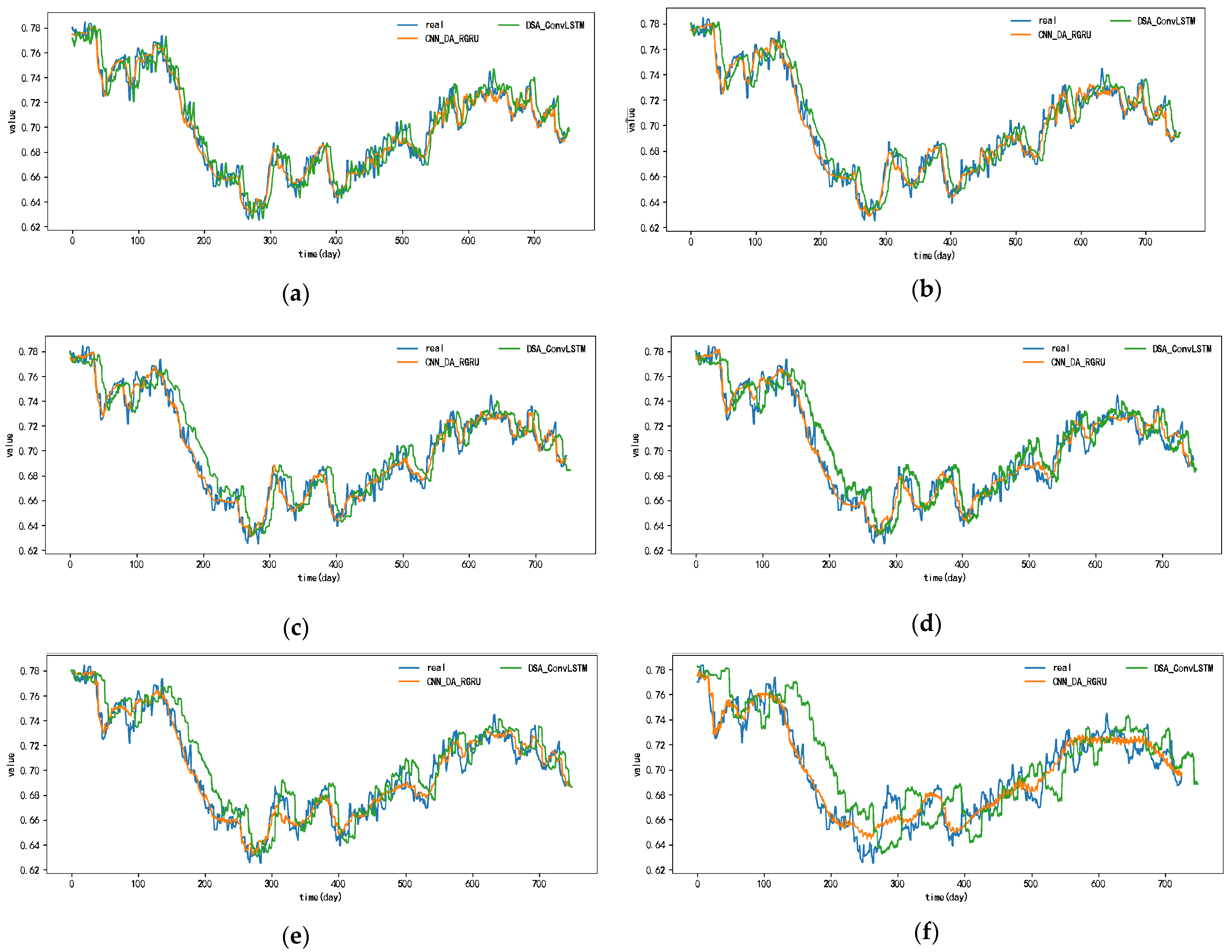
The prediction results of each model for the exchange rate dataset are shown in Figure 11 and Appendix A, Figure A7, Figure A8, Figure A9, Figure A10, Figure A11 and Figure A12. Since the prediction results of the comparative models in this dataset, except for the DSA-Conv-LSTM model, are quite different from the prediction results of the CNN-DA-RGRU model proposed in this paper, only the actual values as well as the comparative prediction results of the DSA-Conv-LSTM and the CNN-DA-RGRU are given in Figure 11. From the figure, it can be seen that the CNN-DA-RGRU model proposed in this paper outperforms DSA-Conv-LSTM when the prediction step size is between three and six steps, and the increase in the step size does not have much effect on the prediction performance of the model in this paper. In the case of multiple step lengths, the model in this paper still has good prediction performance. The reason why the prediction performance of the proposed model in this paper is not as good as that of the second-ranked DSA-Conv-LSTM model when the prediction step size is small is that, although the two models have the same performance in extracting spatial features and important correlation features, the two-phase attentional mechanism of the DSA-Conv-LSTM and the encoder–decoder structure of the LSTM layer make the prediction performance of the DSA-Conv-LSTM model better than that of the second-ranked DSA-Conv-LSTM model when the prediction step length is small. The Conv-LSTM model outperforms the DSA-CONV-LSTM model when the prediction step size is small. However, when the prediction step size gradually increases, the prediction performance of DSA-Conv-LSTM starts to decline due to the accumulation of prediction errors. However, the CNN-DA-RGRU model in this paper deepens the number of network layers due to the presence of residual blocks and residual connections and at the same time reduces the accumulation of errors to a certain extent, which results in a slight decrease in the multi-step prediction performance.
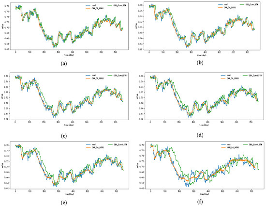
Figure 11.
The 1–6-step real values and forecast results of DSA-Conv-LSTM and proposed CNN-DA-RGRU on the exchange rate dataset, listed as (a) 1-step; (b) 2-step; (c) 3-step; (d) 4-step; (e) 5-step; (f) 6-step.
In summary, the CNN-DA-RGRU model proposed in this paper can better extract the spatial relationship between variables in multivariate series, pay more attention to important features, reduce the network degradation problem caused by residual structure, and increase the path of information flow. The single-step and multi-step forecasting performance of this model on the SML2010 and exchange rate datasets is generally better than other time series forecasting models.
5. Conclusions
Although there are great challenges in multivariable time series prediction for massive time series data, the model proposed in this paper still has good single-step and multi-step prediction ability for multivariable time series. Specifically, the convolution-residual gated recursive hybrid model based on the two-layer attention mechanism proposed in this paper introduces a two-layer attention mechanism with residual block and residual link structure. First, the convolutional module is used to extract the feature space relationship, that is, the relationship between variables. The residual gated loop module extracts the time-dependent features of the time series, deepens the number of network layers, and speeds up the convergence speed. The two-layer attention mechanism eliminates the interference of irrelevant features and extracts features for the model depth. Finally, experiments were conducted on two public datasets: financial and environmental. The experimental results show that the convolution-residual gated recursive hybrid model based on the two-layer attention mechanism proposed in this paper is better than most comparison models in multi-scene tasks. In addition, the model presented in this paper also shows good performance in the face of multi-step prediction of multivariate time series. However, due to the poor feature selection ability of the model, the performance of the model will decrease with the increase in step size in long time step prediction.
In future research on multivariate time series forecasting, the following can be further considered to better achieve accurate multi-step forecasting of multivariate time series:
- (1)
- Adaptive hyper-parameter optimization.
Using deep learning methods to predict tasks often leads to over-fitting due to the large number of parameters [51]. In addition, the hyper-parameters of the model selected in this study are all manually tuned, so it is inevitable to miss the parameters that make the model perform better. In the future, we will further study the adaptive selection of hyper parameters combined with optimization algorithms to reduce the over-fitting phenomenon and the accuracy of parameter selection.
- (2)
- Introduction of long-term serial forecasting model module.
Although the model proposed in this paper has certain advantages over the comparison model, the prediction performance of the model deteriorates with the increase in the prediction step length due to the accumulation of multi-step errors. In future research, we will consider introducing the long-term cash forecasting model technique to reduce the multivariate and multi-step forecasting errors and further improve the performance of the model.
- (3)
- Introduce advanced models such as nonlinear function to function regression model.
The nonlinear function-to-function regression model is a kind of framework of hidden layers composed of continuous neurons [52]. The introduction of this kind of advanced model can better fit the nonlinearity of the data and make the model achieve higher prediction accuracy.
Author Contributions
Methodology, C.C.; software, C.C.; validation, C.C., M.W. and Z.L.; formal analysis, C.C.; data curation, C.C. and Y.S.; writing—original draft preparation, C.C.; writing—review and editing, C.C.; visualization, C.C.; supervision, C.C.; project administration, J.H.; funding acquisition, J.H. All authors have read and agreed to the published version of the manuscript.
Funding
This research received no external funding.
Data Availability Statement
The original data presented in the study can be found in references [39] Zamora-Martinez F, Romeu P, Botella-Rocamora P, Pardo J. On-line learning of indoor temperature forecasting models towards energy efficiency and references [40] Lai G, Chang C, Yang Y et al. Modeling Long and Short-term Temporal Patterns with Deep Neural Networks.
Conflicts of Interest
The authors declare no conflicts of interest.
Appendix A
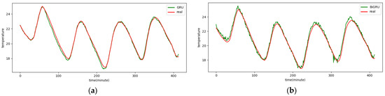
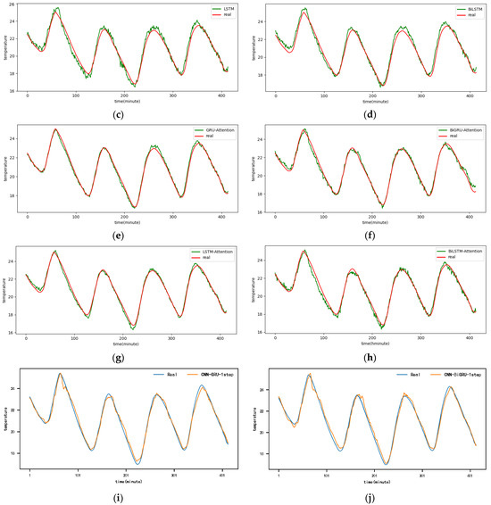
Figure A1.
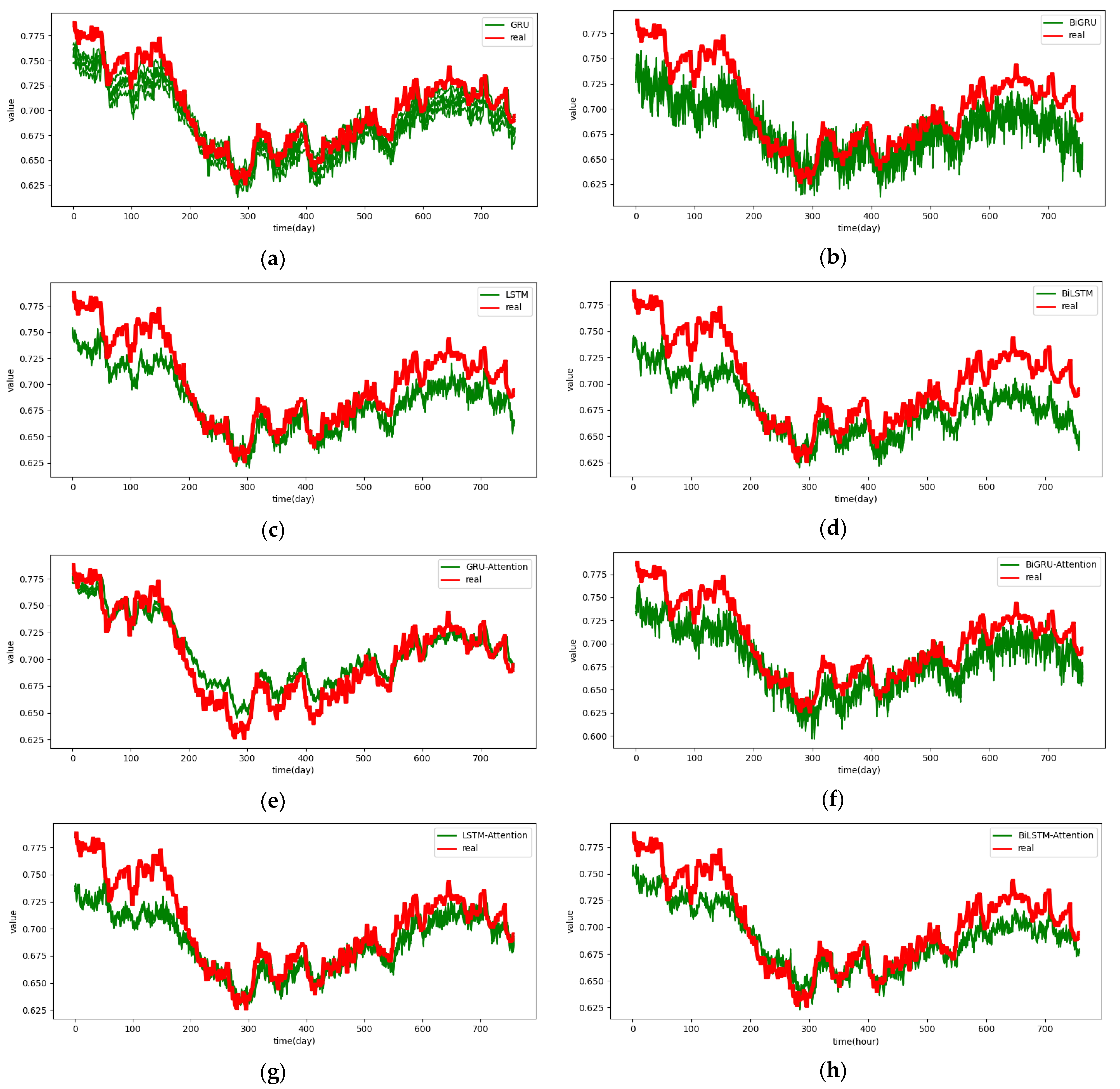
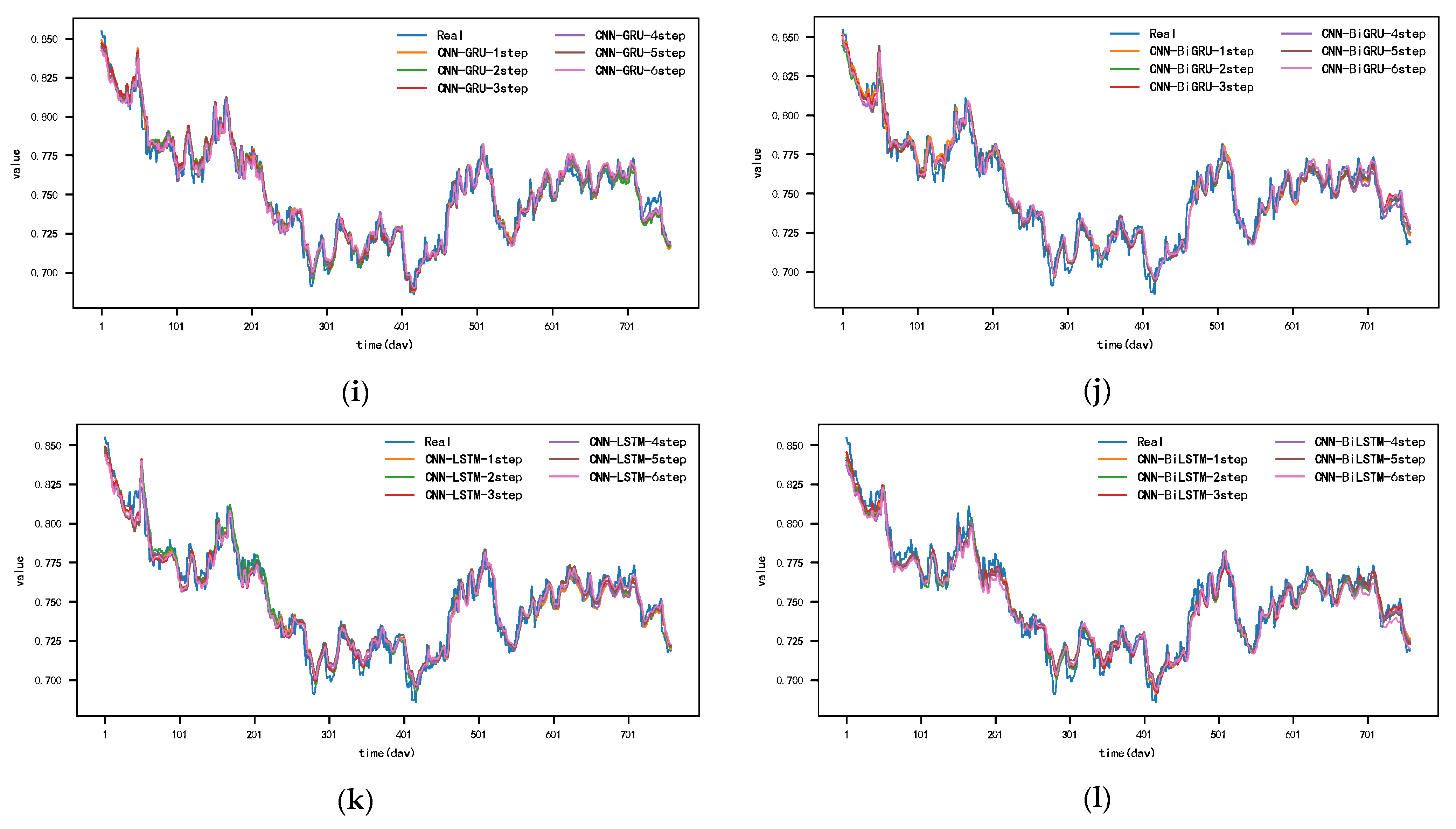
The 1-step real values and forecast results of baselines and proposed CNN-DA-RGRU on SML2010 dataset, listed as (a) GRU; (b) BIGRU; (c) LSTM; (d) BILSTM; (e) GRU-Attention; (f) BIGRU-Attention; (g) LSTM-Attention; (h) BILSTM-Attention; (i) CNN-GRU; (j) CNN-BIGRU; (k) CNN-LSTM; (l) CNN-BILSTM.
Figure A1.
The 1-step real values and forecast results of baselines and proposed CNN-DA-RGRU on SML2010 dataset, listed as (a) GRU; (b) BIGRU; (c) LSTM; (d) BILSTM; (e) GRU-Attention; (f) BIGRU-Attention; (g) LSTM-Attention; (h) BILSTM-Attention; (i) CNN-GRU; (j) CNN-BIGRU; (k) CNN-LSTM; (l) CNN-BILSTM.
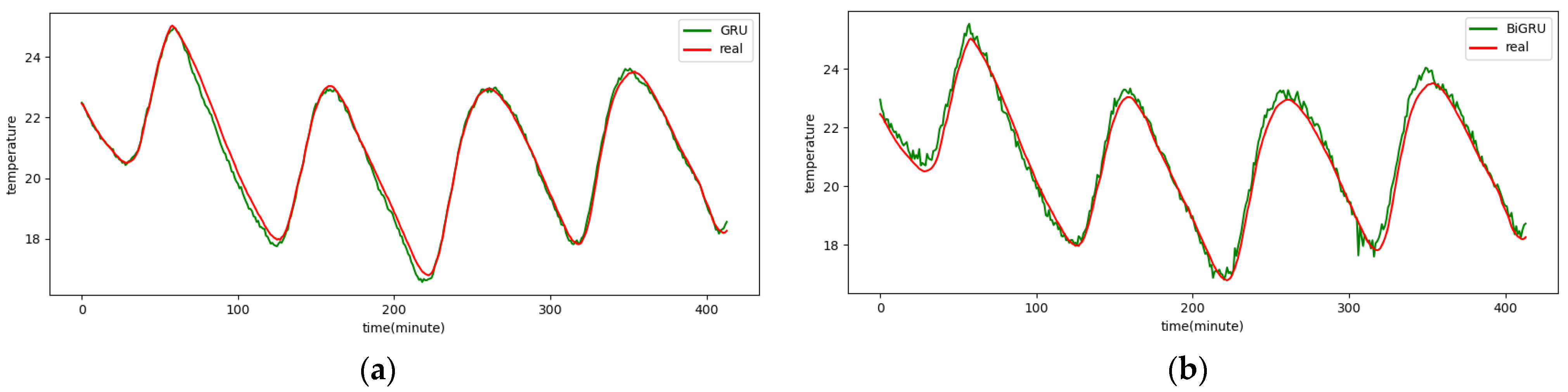
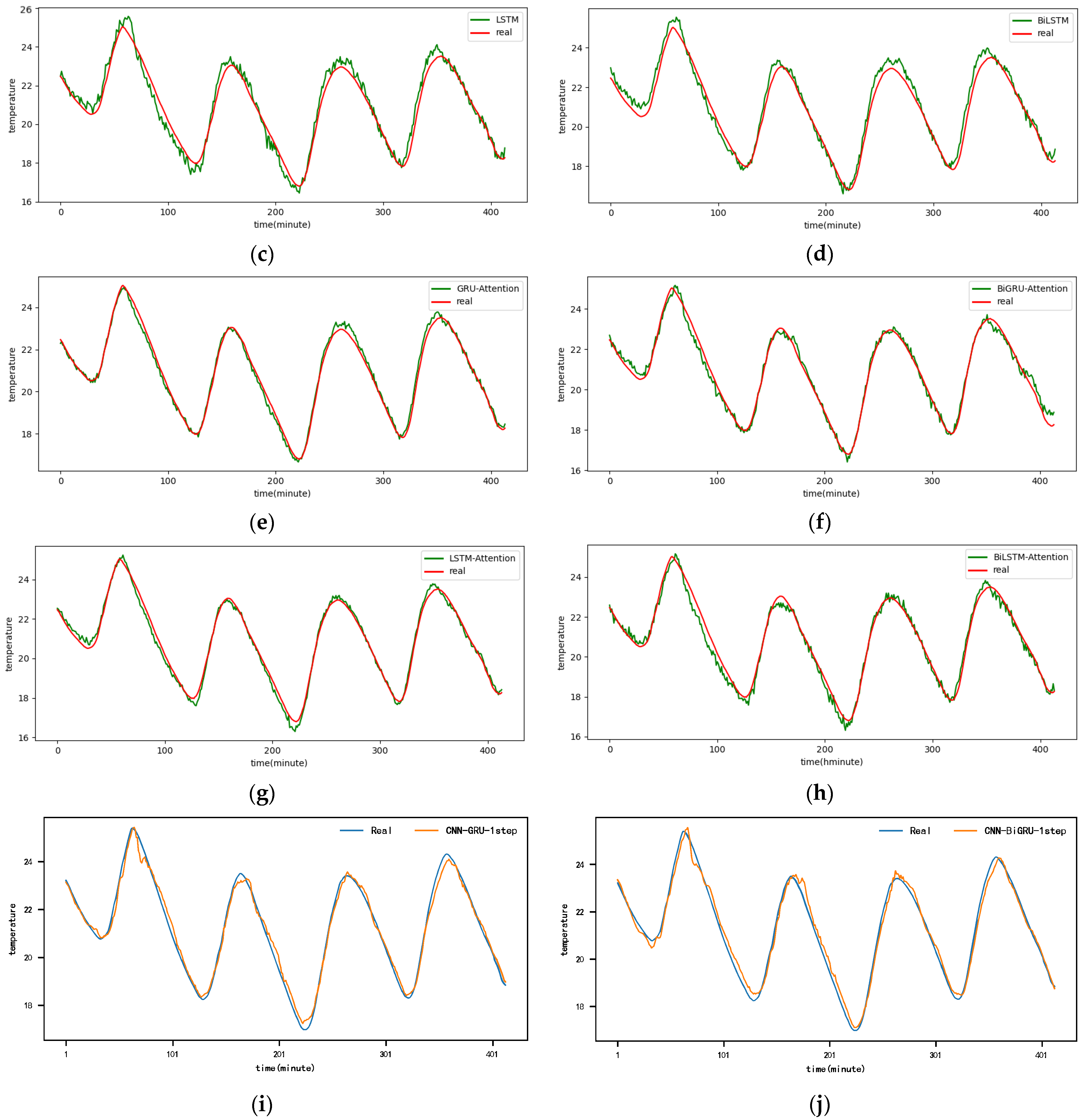
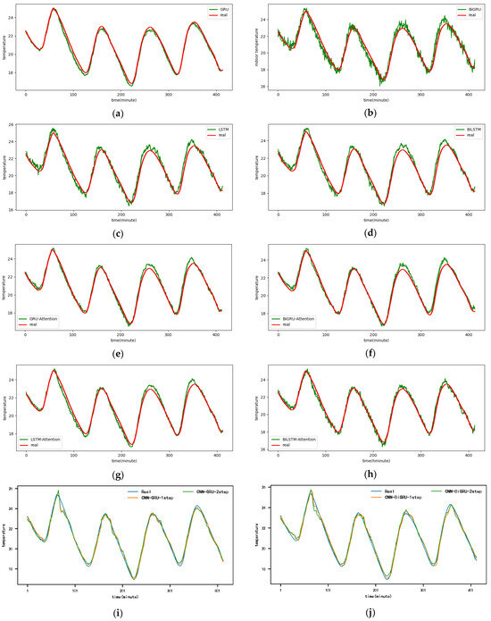
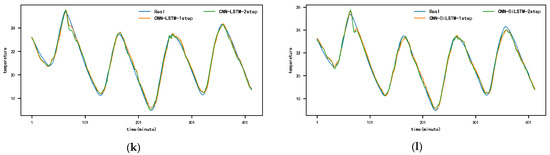
Figure A2.
The 2-step real values and forecast results of baselines and proposed CNN-DA-RGRU on SML2010 dataset, listed as (a) GRU; (b) BIGRU; (c) LSTM; (d) BILSTM; (e) GRU-Attention; (f) BIGRU-Attention; (g) LSTM-Attention; (h) BILSTM-Attention; (i) CNN-GRU; (j) CNN-BIGRU; (k) CNN-LSTM; (l) CNN-BILSTM.
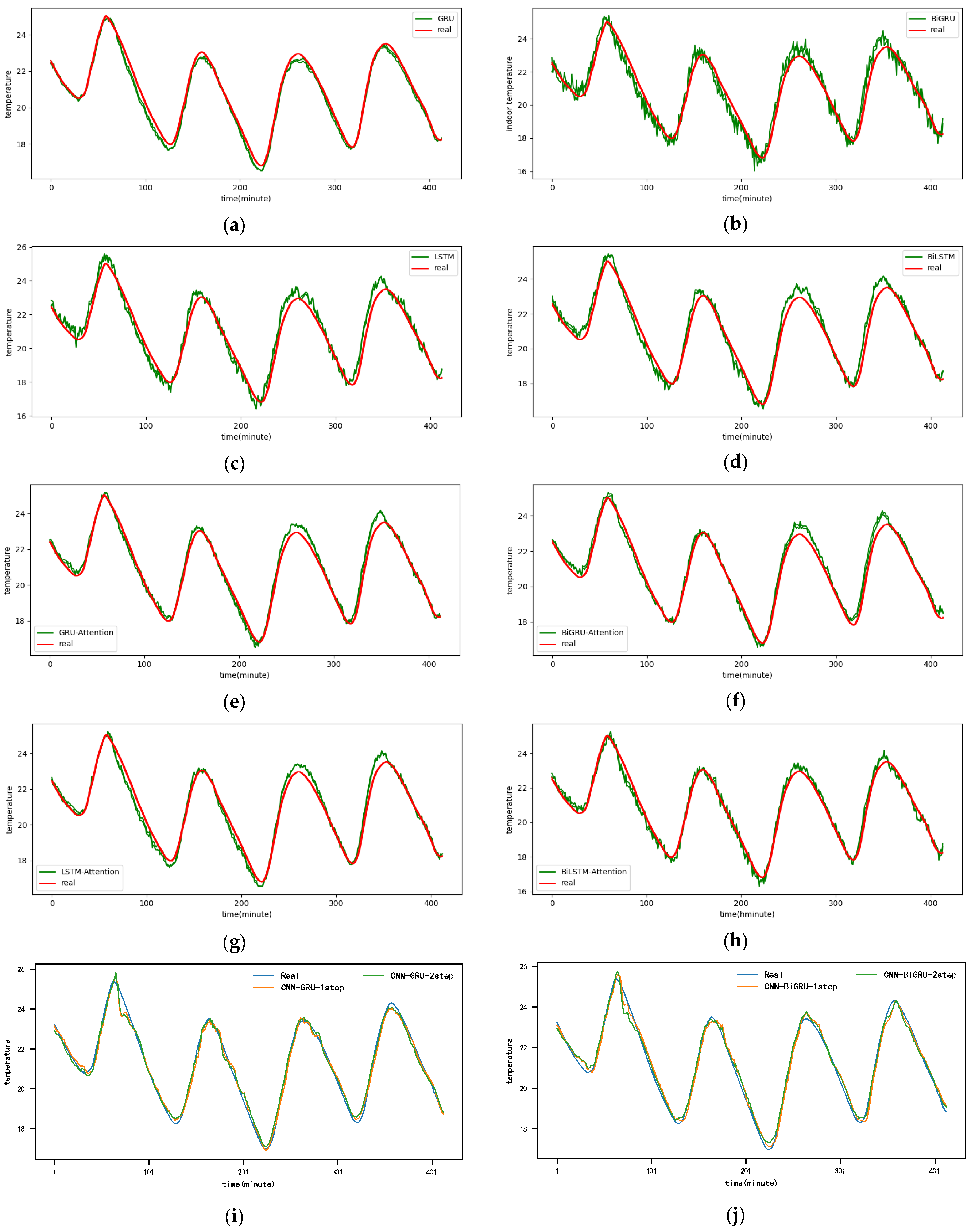
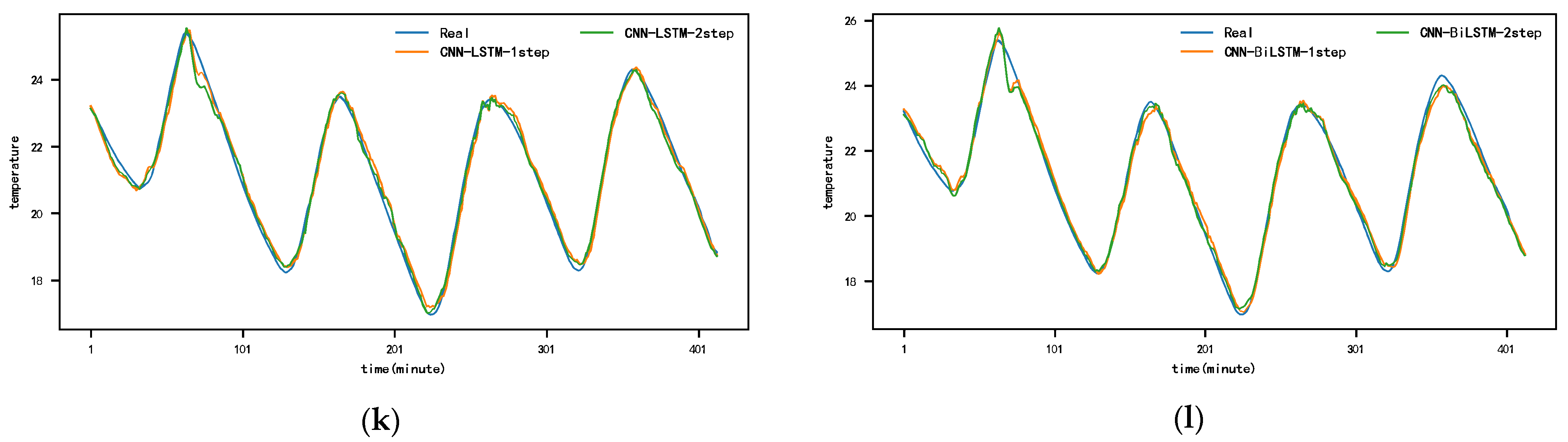
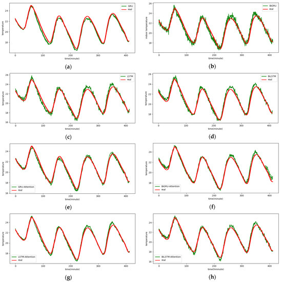
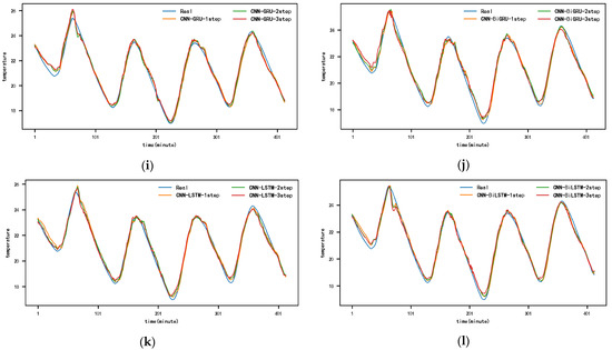
Figure A3.
The 3-step real values and forecast results of baselines and proposed CNN-DA-RGRU on SML2010 dataset, listed as (a) GRU; (b) BIGRU; (c) LSTM; (d) BILSTM; (e) GRU-Attention; (f) BIGRU-Attention; (g) LSTM-Attention; (h) BILSTM-Attention; (i) CNN-GRU; (j) CNN-BIGRU; (k) CNN-LSTM; (l) CNN-BILSTM.
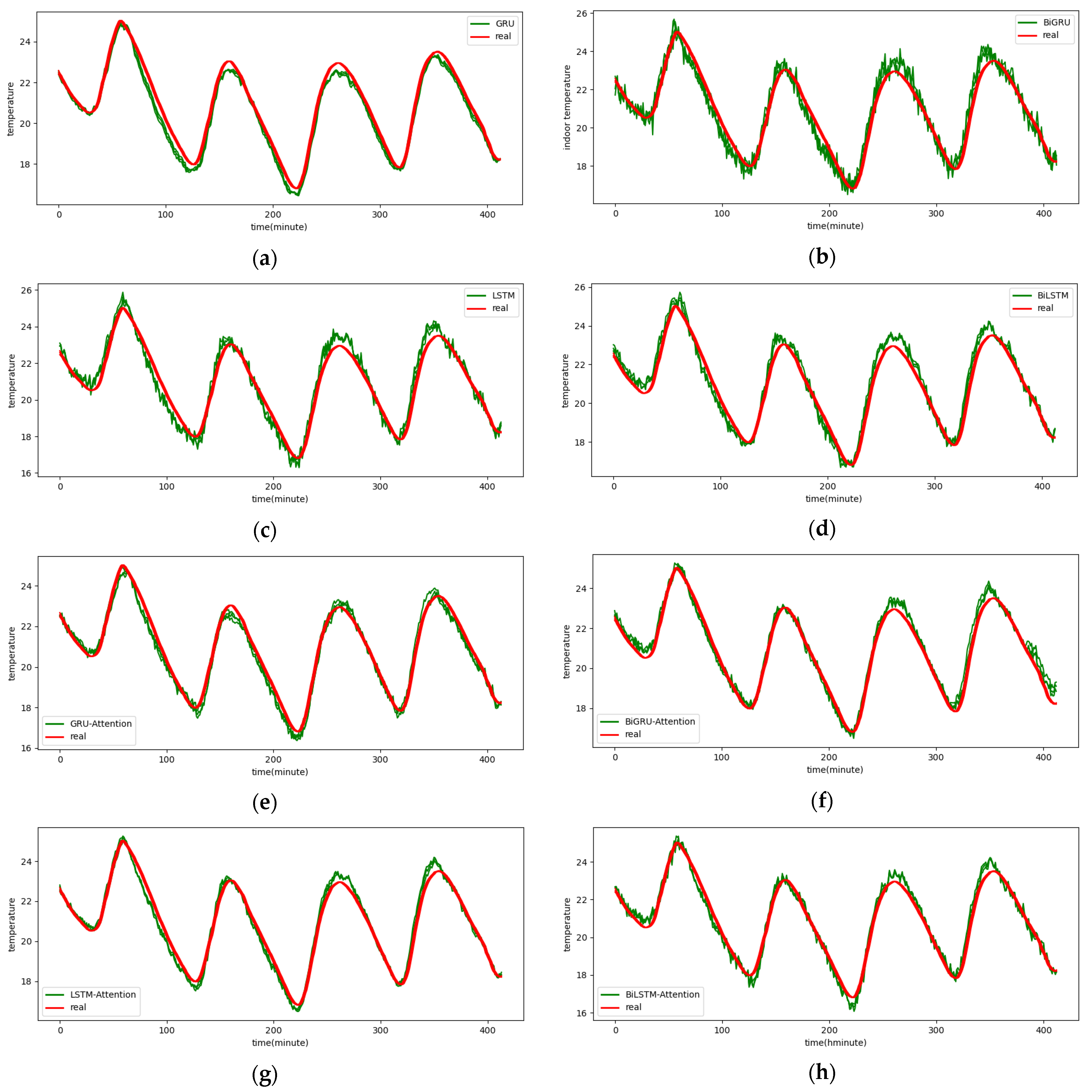
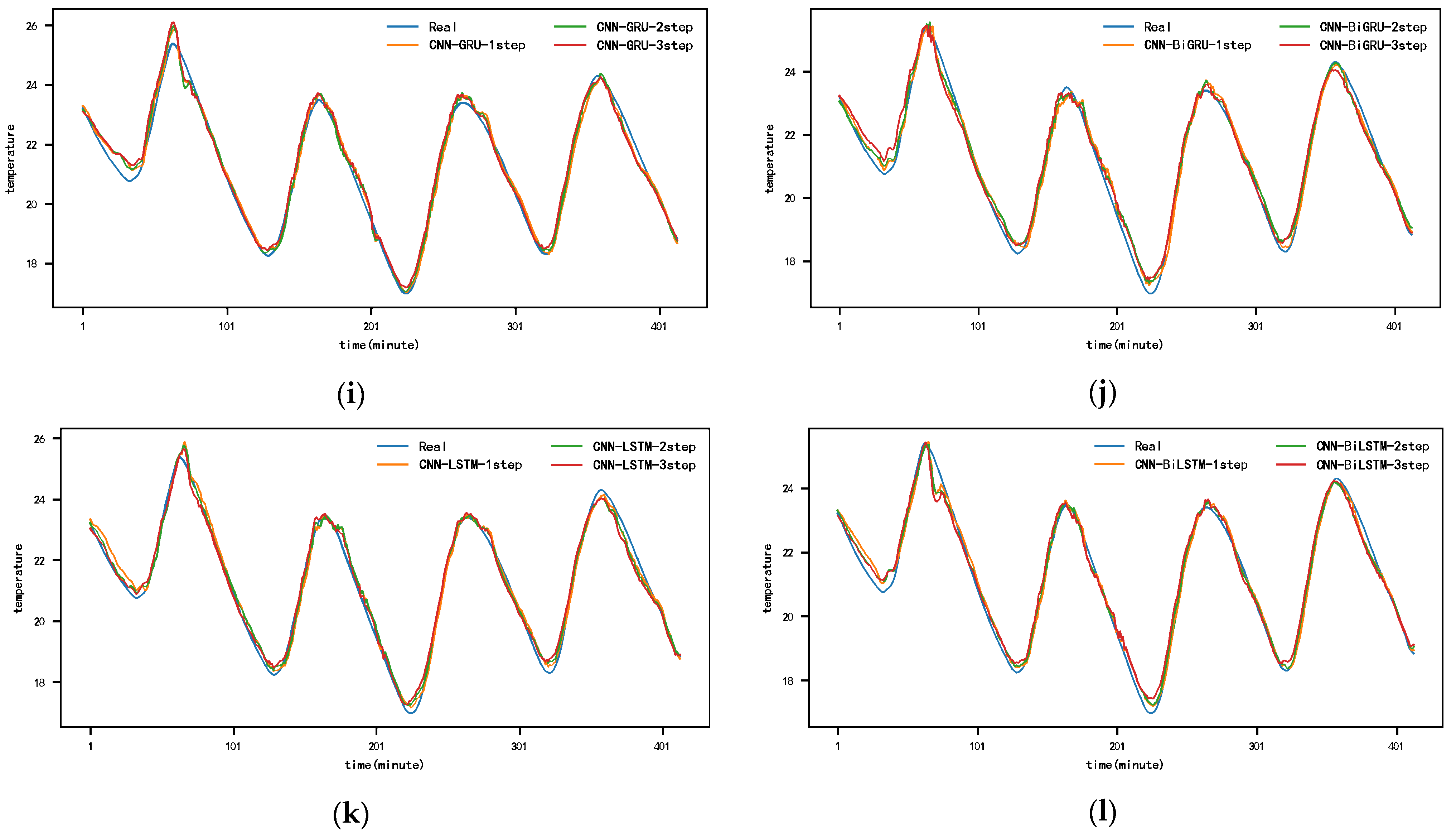
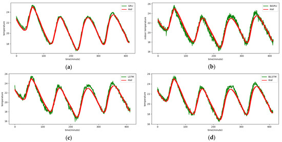
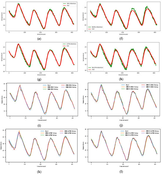
Figure A4.
The 4-step real values and forecast results of baselines and proposed CNN-DA-RGRU on SML2010 dataset, listed as (a) GRU; (b) BIGRU; (c) LSTM; (d) BILSTM; (e) GRU-Attention; (f) BIGRU-Attention; (g) LSTM-Attention; (h) BILSTM-Attention; (i) CNN-GRU; (j) CNN-BIGRU; (k) CNN-LSTM; (l) CNN-BILSTM.
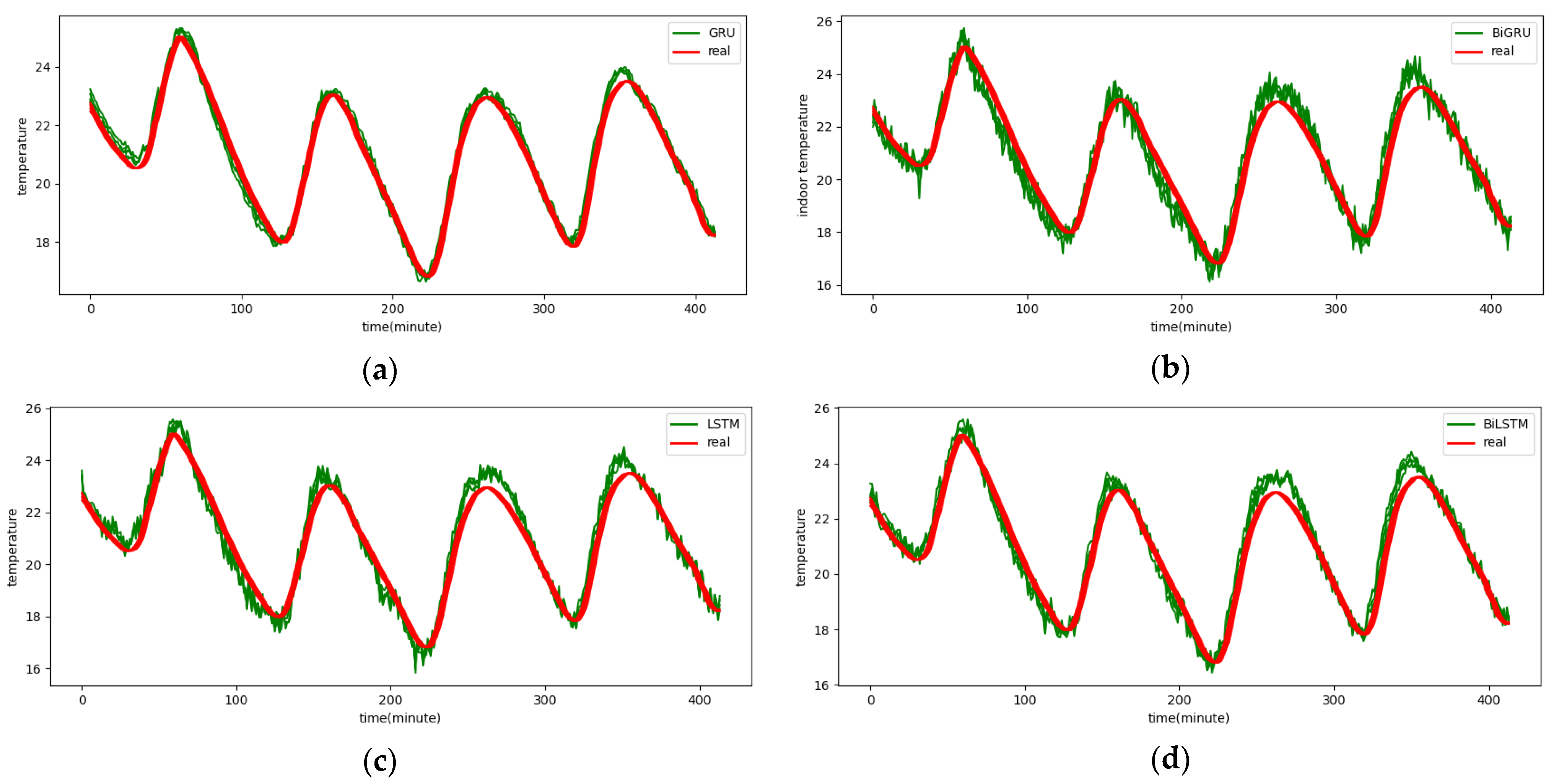
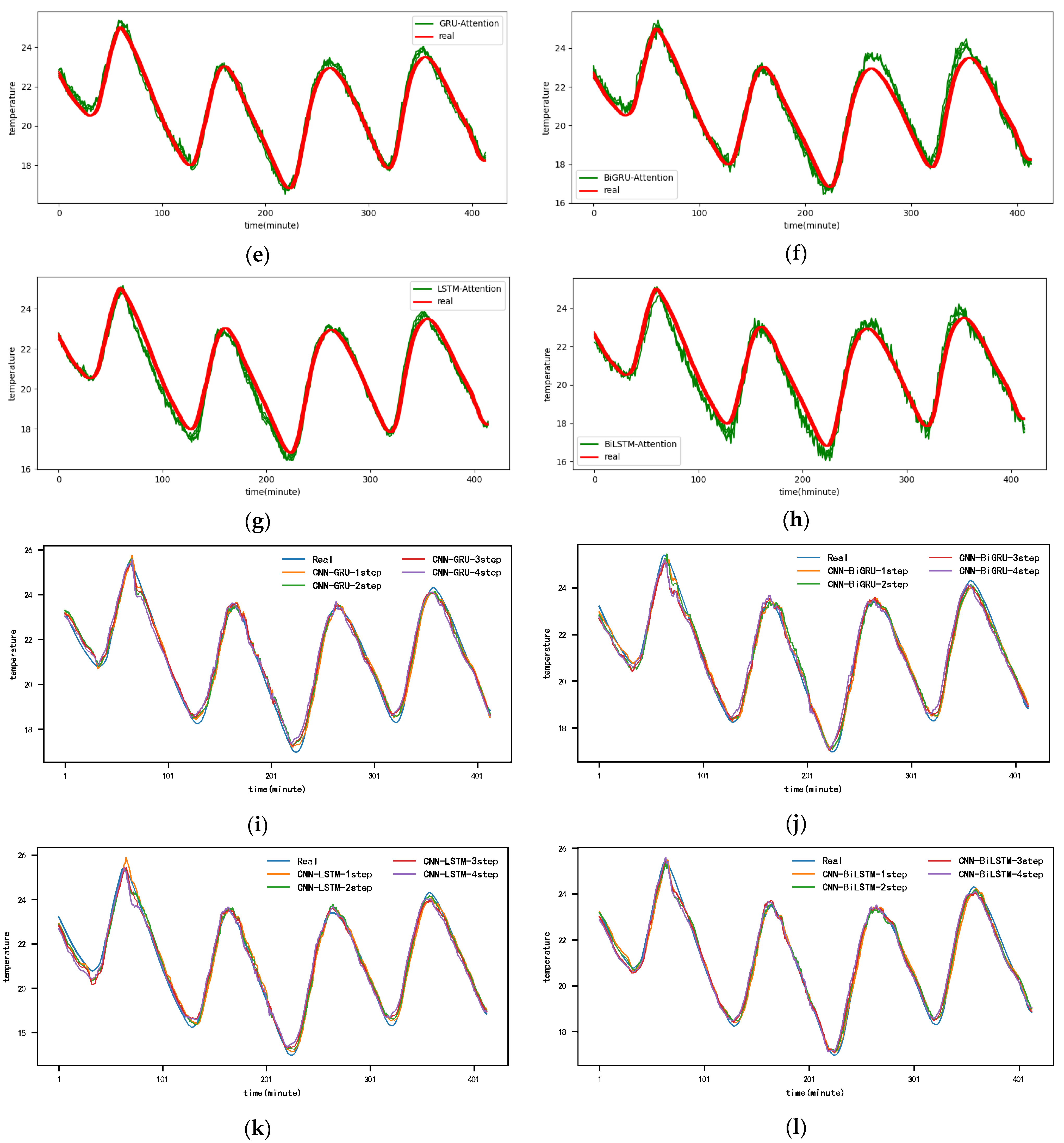
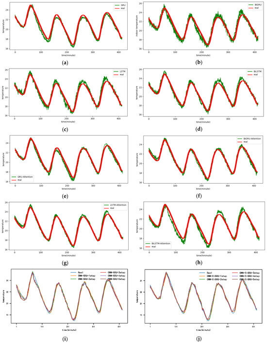

Figure A5.
The 5-step real values and forecast results of baselines and proposed CNN-DA-RGRU on SML2010 dataset, listed as (a) GRU; (b) BIGRU; (c) LSTM; (d) BILSTM; (e) GRU-Attention; (f) BIGRU-Attention; (g) LSTM-Attention; (h) BILSTM-Attention; (i) CNN-GRU; (j) CNN-BIGRU; (k) CNN-LSTM; (l) CNN-BILSTM.
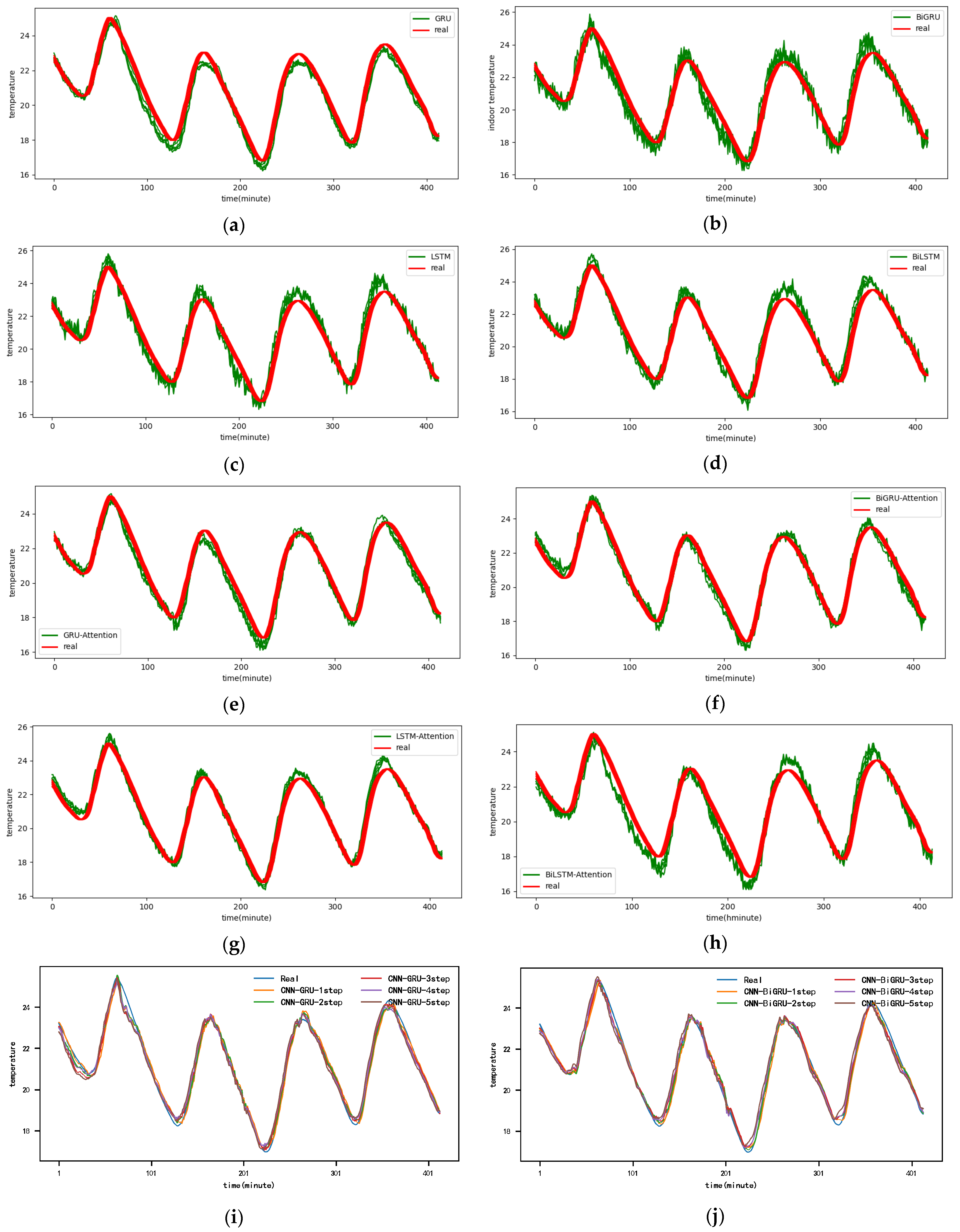
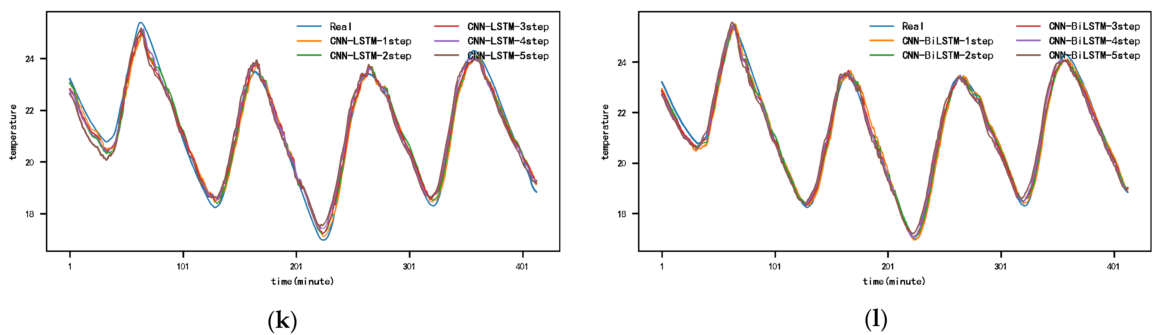
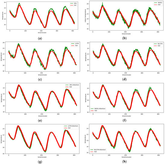
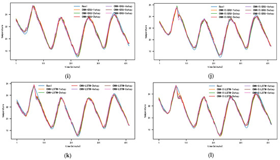
Figure A6.
The 6-step real values and forecast results of baselines and proposed CNN-DA-RGRU on SML2010 dataset, listed as (a) GRU; (b) BIGRU; (c) LSTM; (d) BILSTM; (e) GRU-Attention; (f) BIGRU-Attention; (g) LSTM-Attention; (h) BILSTM-Attention; (i) CNN-GRU; (j) CNN-BIGRU; (k) CNN-LSTM; (l) CNN-BILSTM.
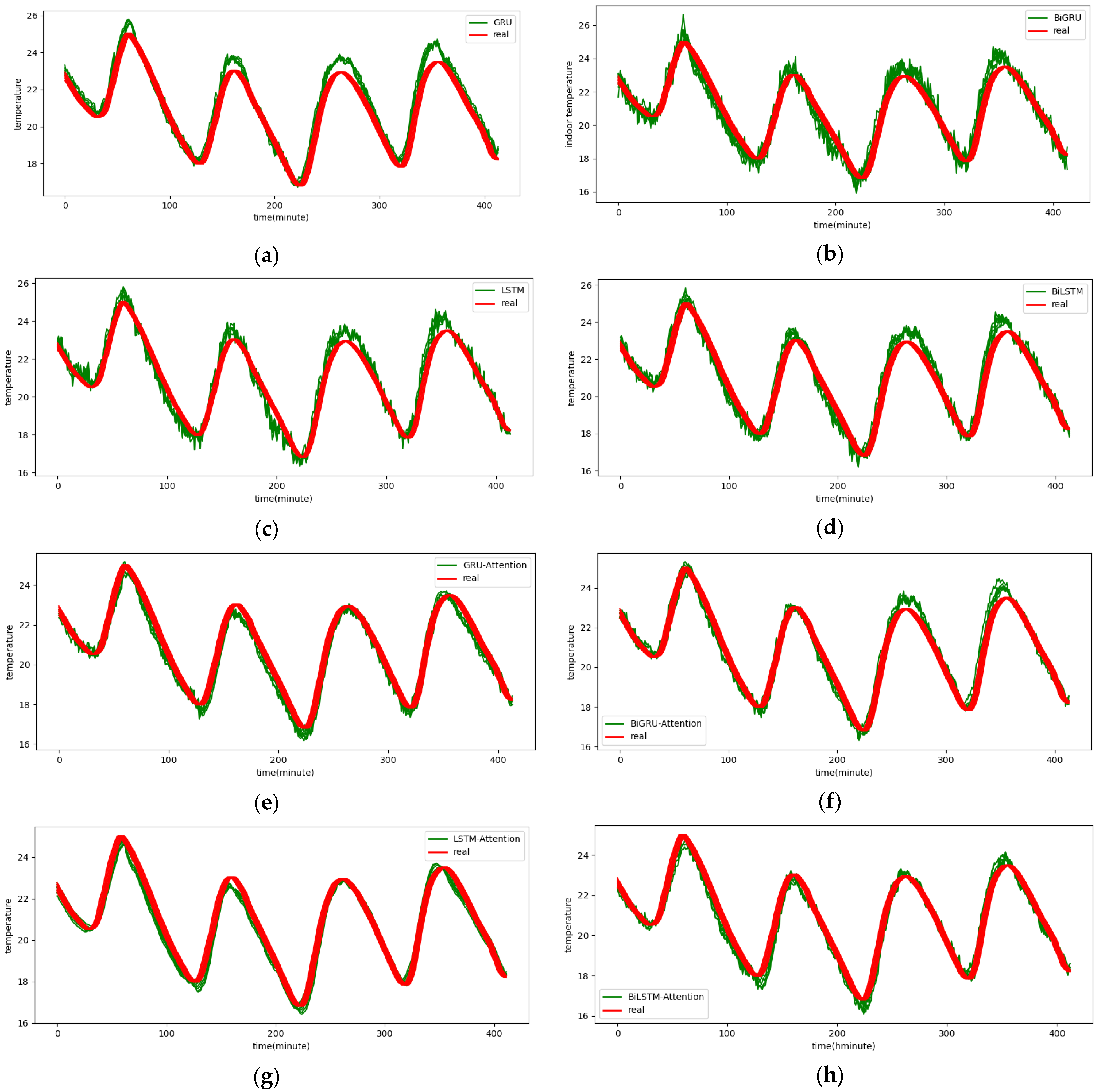
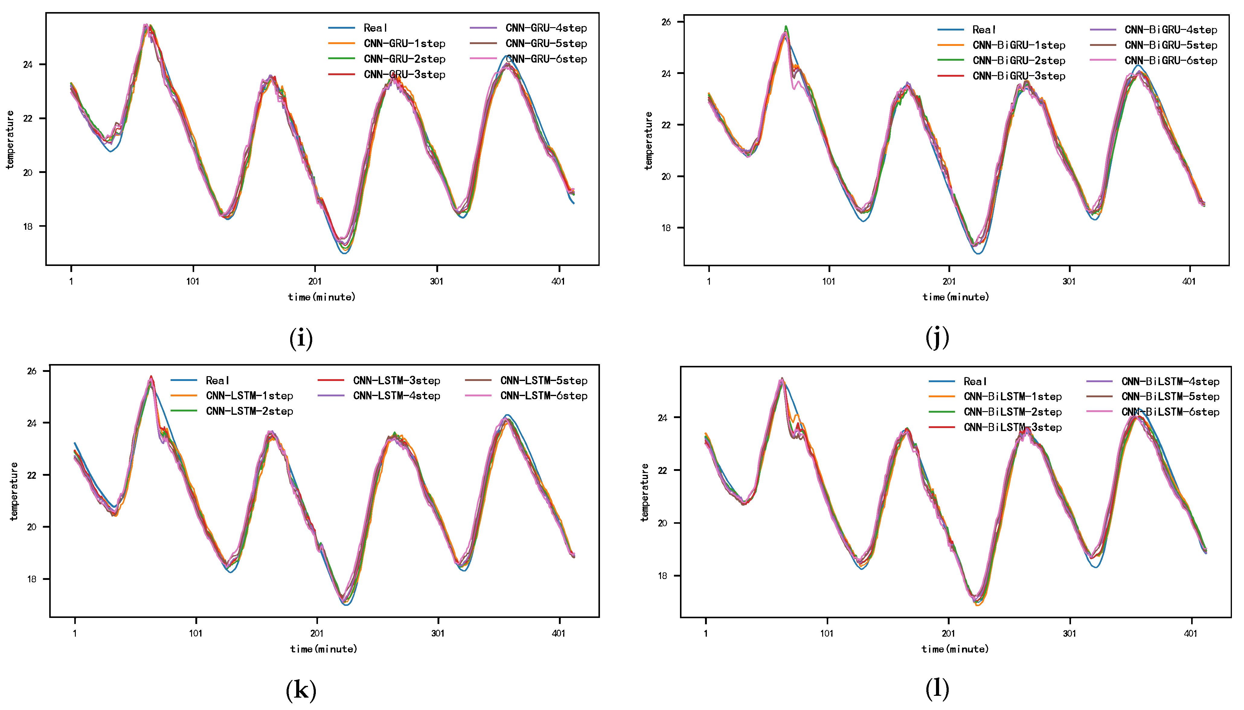
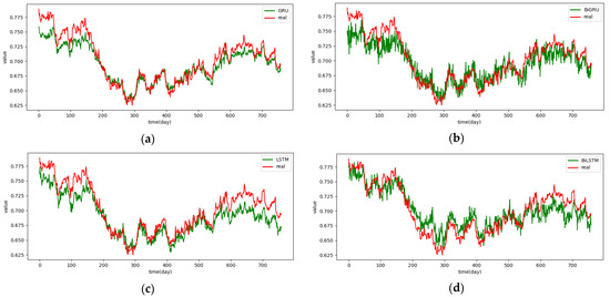
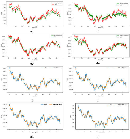
Figure A7.
The 1-step real values and forecast results of baselines and proposed CNN-DA-RGRU on the exchange rate dataset, listed as (a) GRU; (b) BIGRU; (c) LSTM; (d) BILSTM; (e) GRU-Attention; (f) BIGRU-Attention; (g) LSTM-Attention; (h) BILSTM-Attention; (i) CNN-GRU; (j) CNN-BIGRU; (k) CNN-LSTM; (l) CNN-BILSTM.
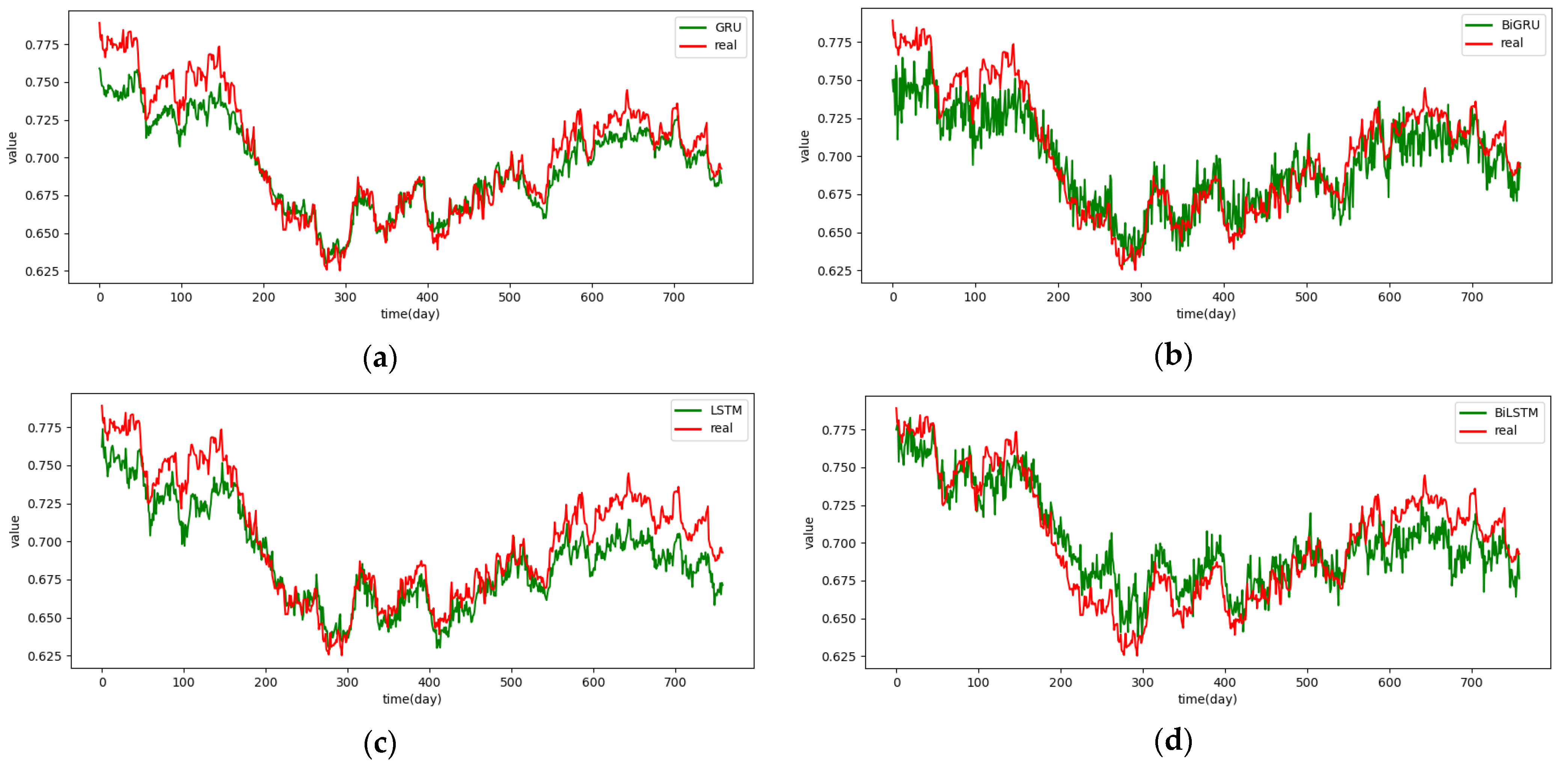
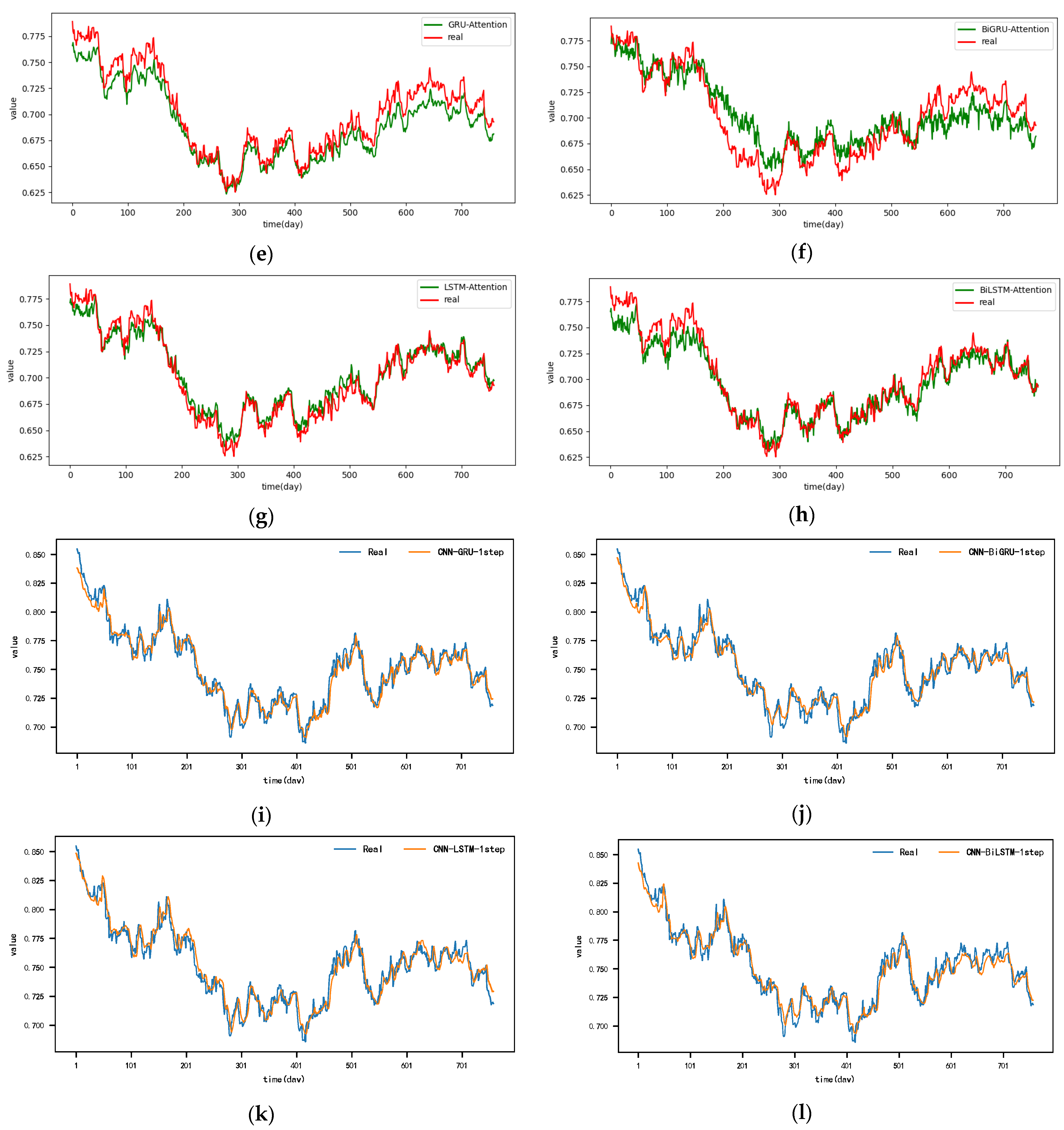
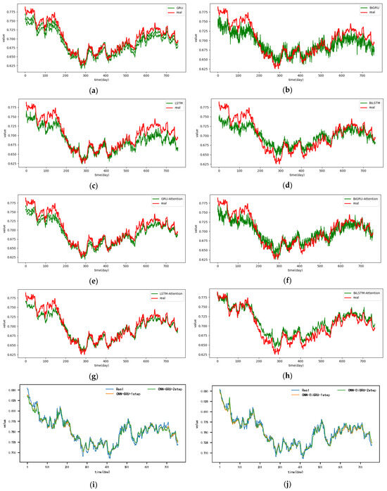
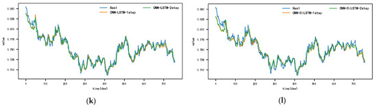
Figure A8.
The 2-step real values and forecast results of baselines and proposed CNN-DA-RGRU on the exchange rate dataset, listed as (a) GRU; (b) BIGRU; (c) LSTM; (d) BILSTM; (e) GRU-Attention; (f) BIGRU-Attention; (g) LSTM-Attention; (h) BILSTM-Attention; (i) CNN-GRU; (j) CNN-BIGRU; (k) CNN-LSTM; (l) CNN-BILSTM.
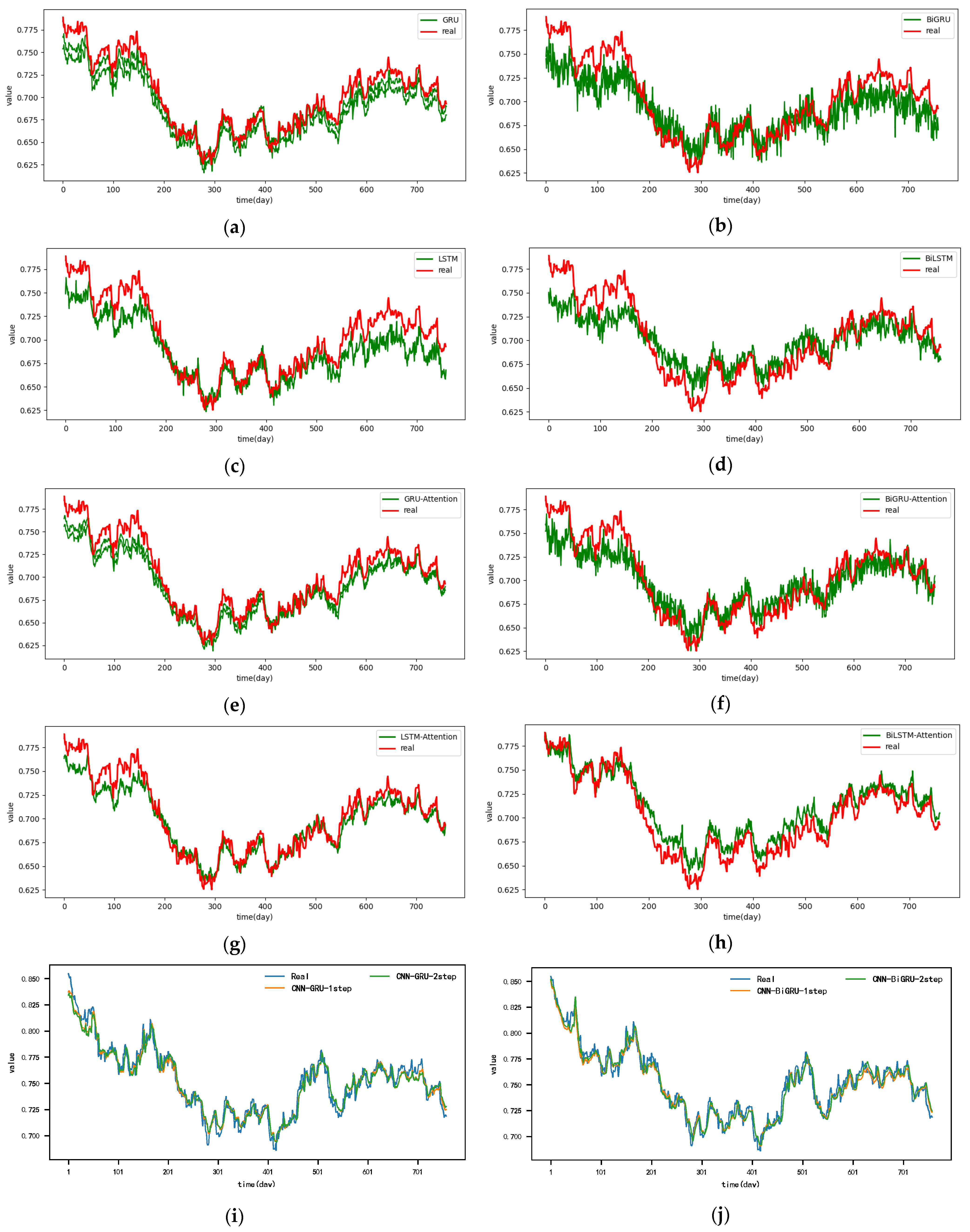
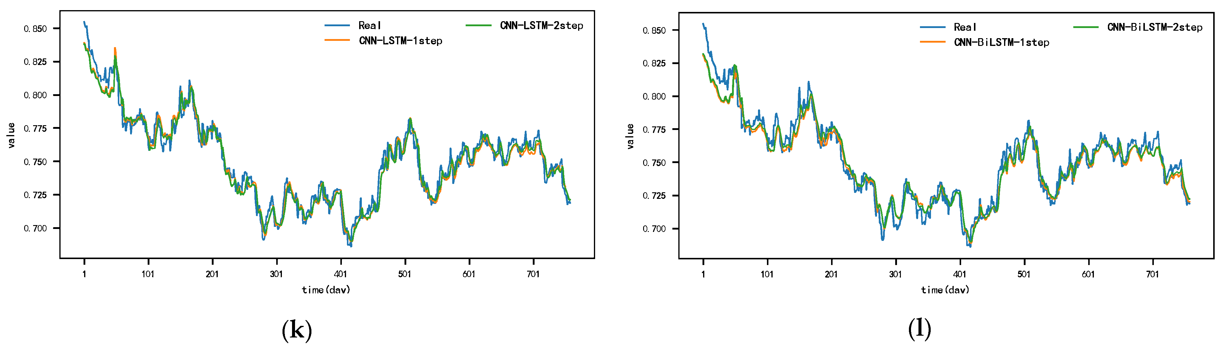
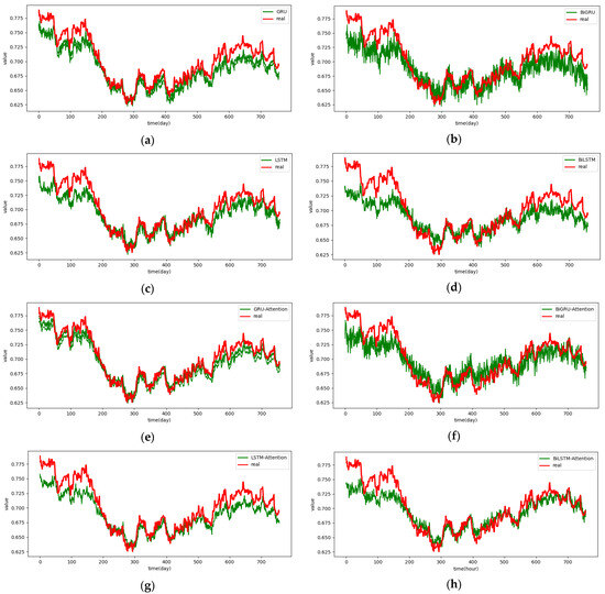
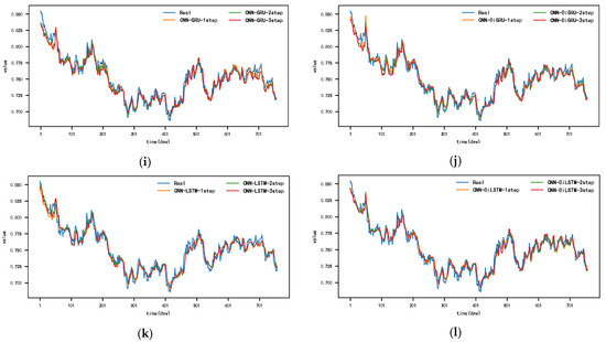
Figure A9.
The 3-step real values and forecast results of baselines and proposed CNN-DA-RGRU on the exchange rate dataset, listed as (a) GRU; (b) BIGRU; (c) LSTM; (d) BILSTM; (e) GRU-Attention; (f) BIGRU-Attention; (g) LSTM-Attention; (h) BILSTM-Attention; (i) CNN-GRU; (j) CNN-BIGRU; (k) CNN-LSTM; (l) CNN-BILSTM.
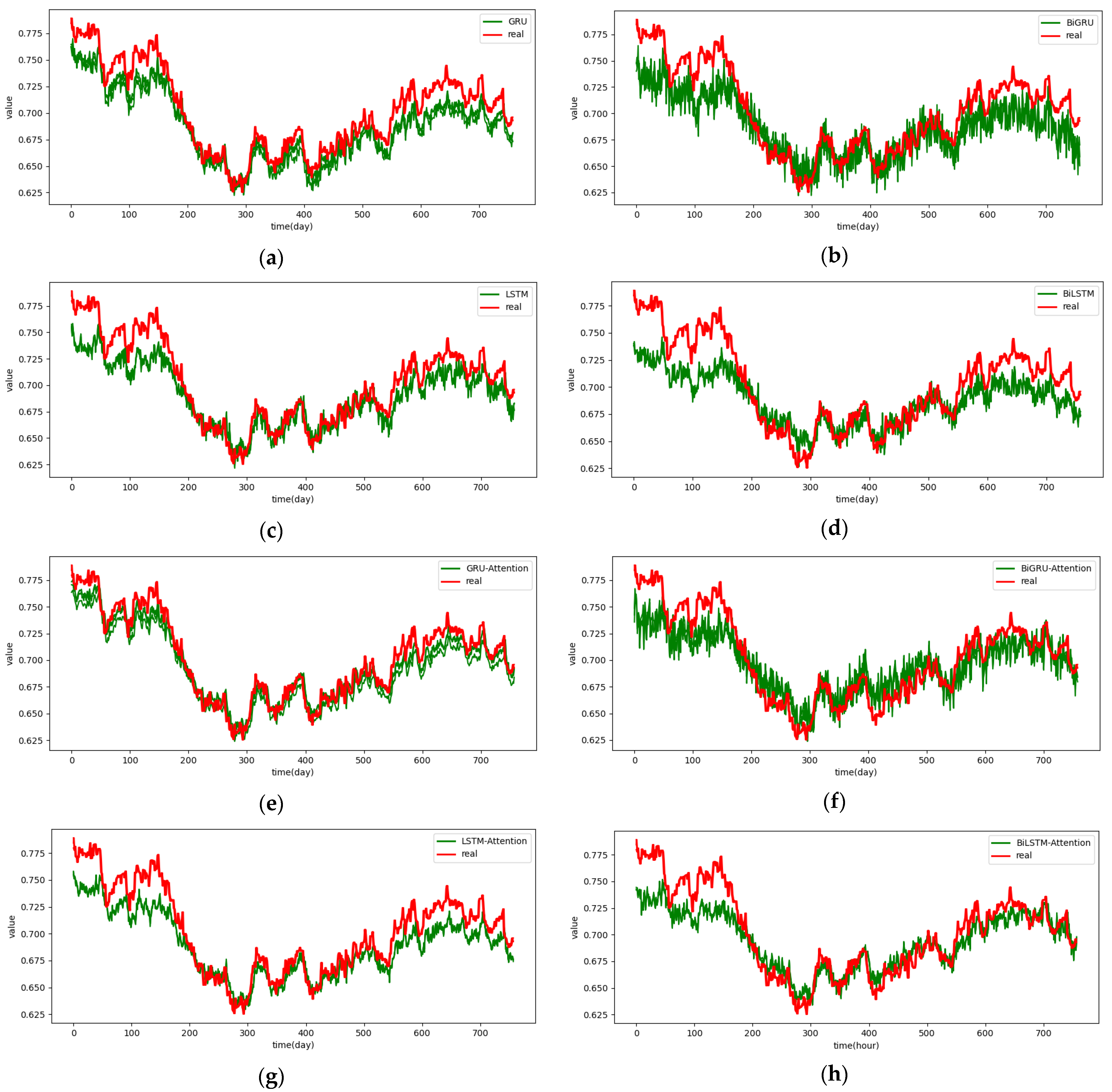
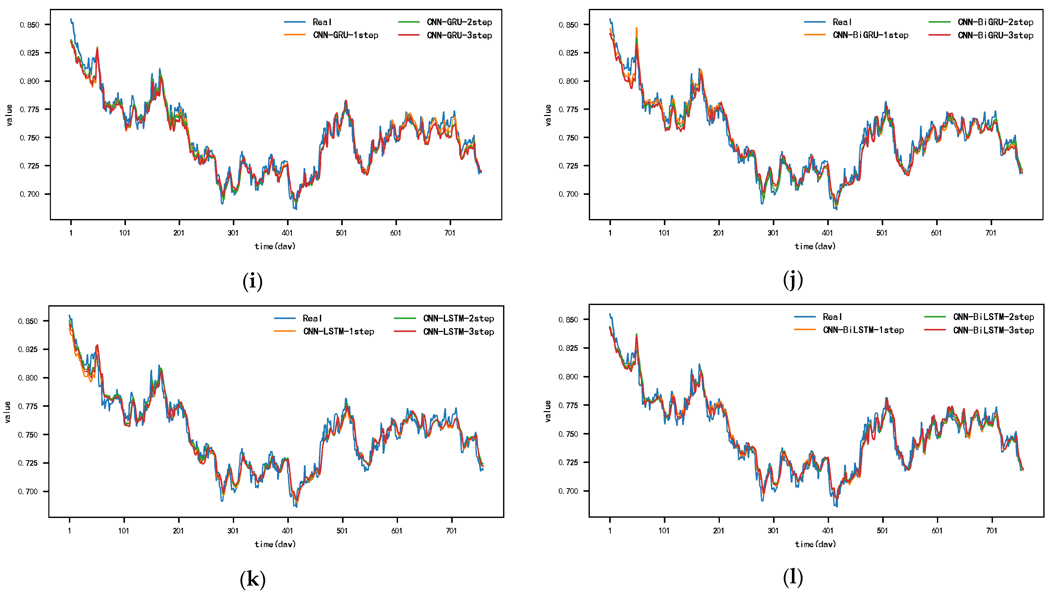
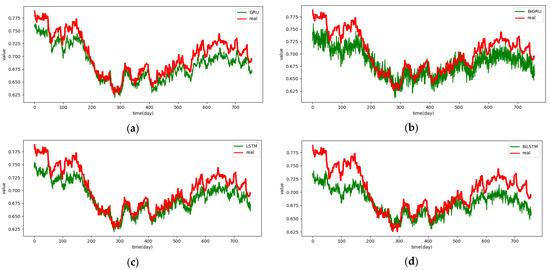
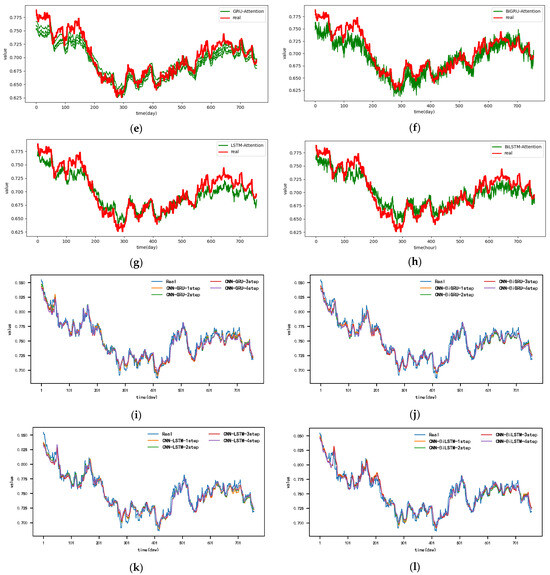
Figure A10.
The 4-step real values and forecast results of baselines and proposed CNN-DA-RGRU on the exchange rate dataset, listed as (a) GRU; (b) BIGRU; (c) LSTM; (d) BILSTM; (e) GRU-Attention; (f) BIGRU-Attention; (g) LSTM-Attention; (h) BILSTM-Attention; (i) CNN-GRU; (j) CNN-BIGRU; (k) CNN-LSTM; (l) CNN-BILSTM.
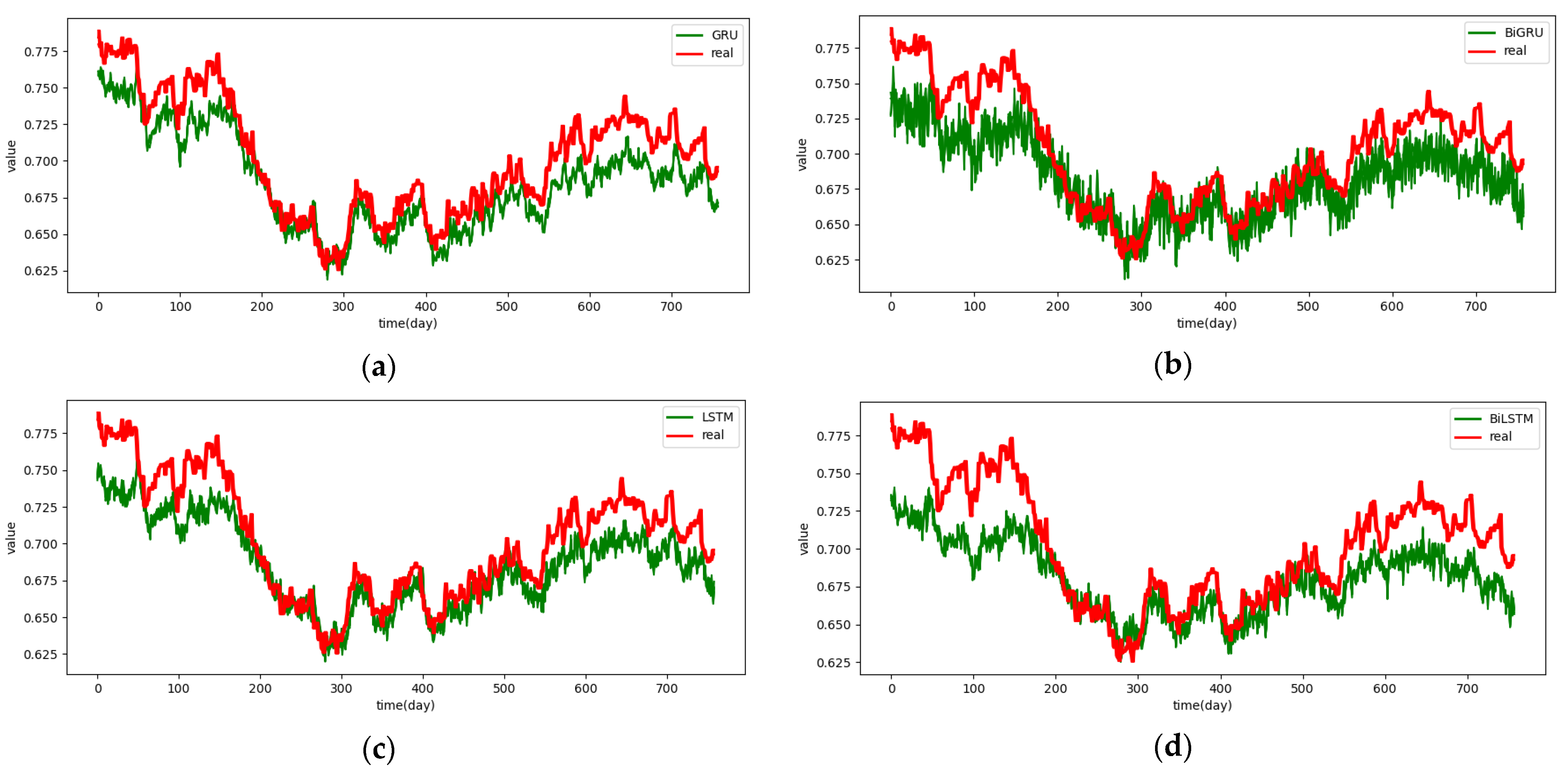
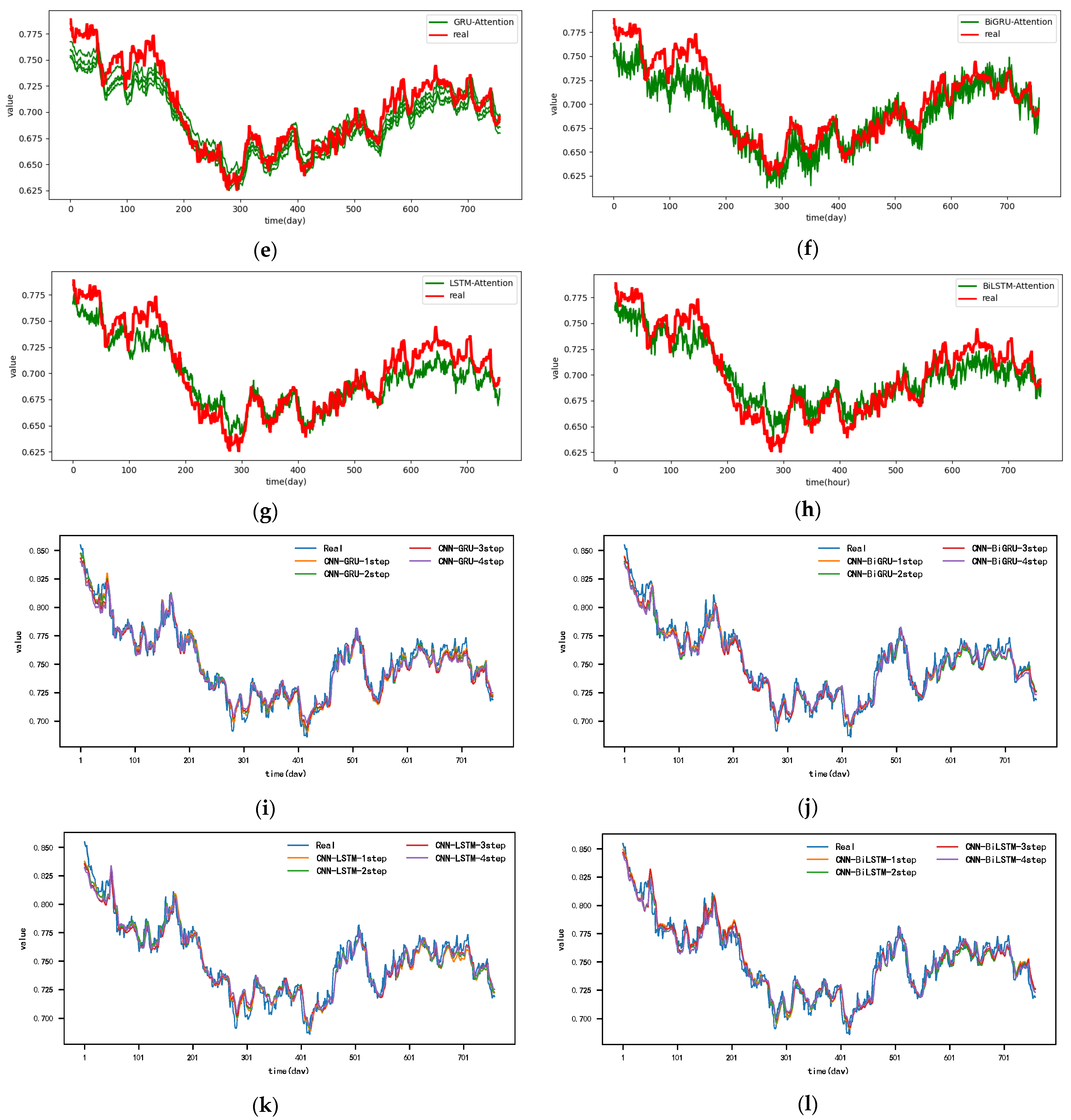
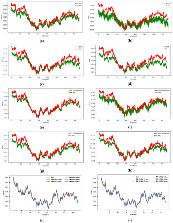
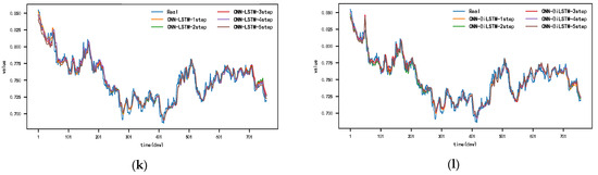
Figure A11.
The 5-step real values and forecast results of baselines and proposed CNN-DA-RGRU on the exchange rate dataset, listed as (a) GRU; (b) BIGRU; (c) LSTM; (d) BILSTM; (e) GRU-Attention; (f) BIGRU-Attention; (g) LSTM-Attention; (h) BILSTM-Attention; (i) CNN-GRU; (j) CNN-BIGRU; (k) CNN-LSTM; (l) CNN-BILSTM.
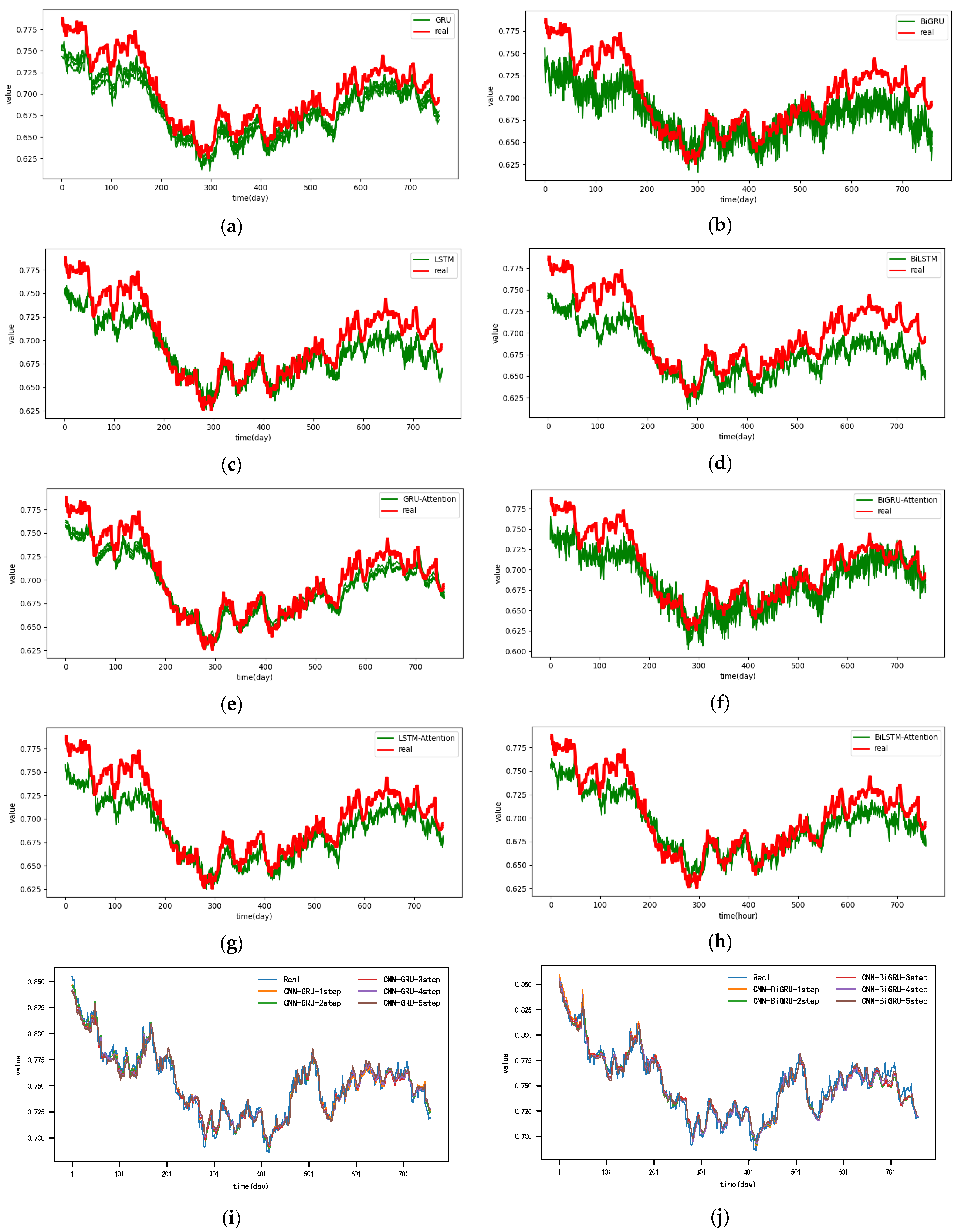
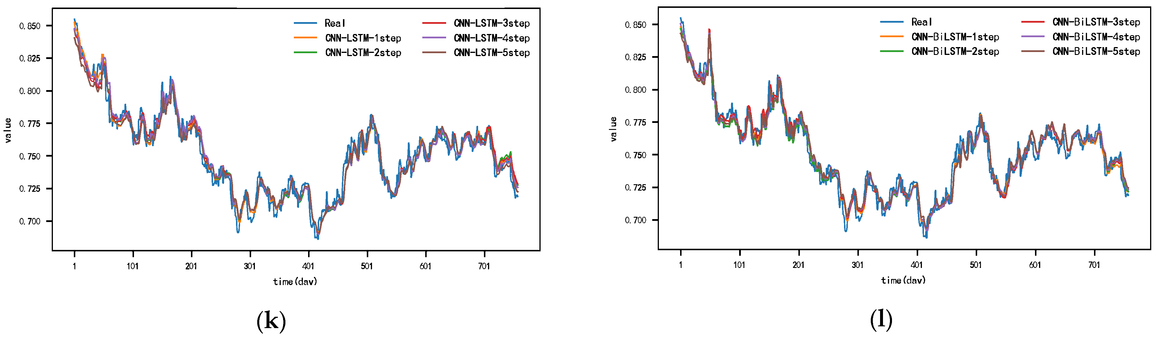
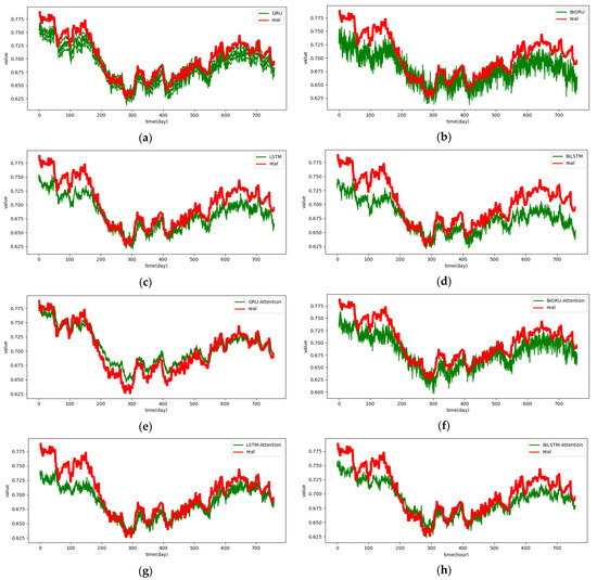
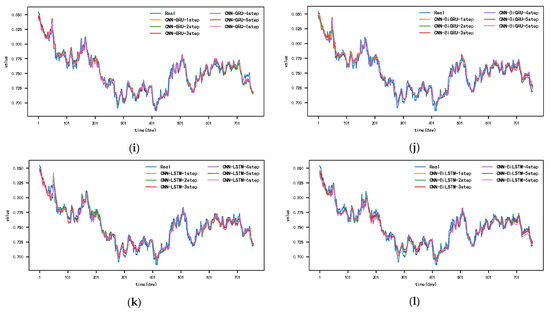
Figure A12.
The 6-step real values and forecast results of baselines and proposed CNN-DA-RGRU on the exchange rate dataset, listed as (a) GRU; (b) BIGRU; (c) LSTM; (d) BILSTM; (e) GRU-Attention; (f) BIGRU-Attention; (g) LSTM-Attention; (h) BILSTM-Attention; (i) CNN-GRU; (j) CNN-BIGRU; (k) CNN-LSTM; (l) CNN-BILSTM.
References
- Yin, H.; Qi, H.; Xu, J.; Huang, W.; Song, X. Generalized Framework for Similarity Measure of Time Series. Math. Probl. Eng. 2014, 16, 572124. [Google Scholar] [CrossRef]
- Kim, T.; Cho, S. Predicting Residential Energy Consumption Using CNN-LSTM Neural Networks. Energy 2019, 182, 72–81. [Google Scholar] [CrossRef]
- Sun, K.; Zhu, Z.; Lin, Z. ADAGCN: Adaboosting Graph Convolutional Networks into Deep Models. In Proceedings of the 9th International Conference of Learning Representations (ICLR 2021), Virtual Event, Austria, 3–7 May 2021. [Google Scholar]
- Kim, D.; Kim, K. A Convolutional Transformer Model for Multivariate Time Series Prediction. IEEE Access 2022, 10, 101319–101329. [Google Scholar] [CrossRef]
- Yuan, H.; Kong, Z.; Zhao, J.; Xiong, J. Applications of Time-Series Hesitation Fuzzy Soft Sets in Group Decision Making. In Proceedings of the 31st Chinese Control and Decision Conference (CCDC 2019), Nanchang, China, 3–5 June 2019. [Google Scholar]
- Lucia, C.; Samia, S.; Saleem, U.; Seyedali, M.; Hafeez, U.; Muhammad, U. Predicting Household Electric Power Consumption Using Multi-step Time Series with Convolutional LSTM. Big Data Res. 2023, 31, 100360. [Google Scholar]
- Peng, L.; Wang, L.; Ai, X.; Zeng, Y. Forecasting Tourist Arrivals via Random Forest and Long Short-term Memory. Cogn. Comput. 2021, 13, 125–138. [Google Scholar] [CrossRef]
- Chen, T.; Yin, H.; Chen, H.; Wu, L.; Wang, H.; Zhou, X.; Li, X. TADA: Trend Alignment with Dual-Attention Multi-task Recurrent Neural Networks for Sales Prediction. In Proceedings of the IEEE International Conference on Data Mining (ICDM 2018), Sentosa, Singapore, 17–20 November 2018. [Google Scholar]
- Wang, B.; Li, T.; Yan, Z.; Zhang, G.; Lu, J. DeepPIPE: A Distribution-free Uncertainty Quantification Approach for Time Series Forecasting. Neurocomputing 2020, 397, 11–19. [Google Scholar] [CrossRef]
- Xiao, Y.; Yin, H.; Xia, K.; Zhang, Y.; Qi, H. Utilization of CNN-LSTM Model in Prediction of Multivariate Time Series for UCG. In Proceedings of the Machine Learning for Cyber Security (ML4CS 2020), Guangzhou, China, 8–10 October 2020. [Google Scholar]
- Li, Y.; Zhu, Z.; Kong, D.; Han, H.; Zhao, Y. EA-LSTM: Evolutionary Attention-based LSTM for Time Series Prediction. Knowl. Based Syst. 2019, 181, 104785. [Google Scholar] [CrossRef]
- Liu, Y.; Gong, C.; Yang, L.; Chen, Y. DSTP-RNN: A Dual-stage Two-phase Attention-based Recurrent Neural Network for Long-term and Multivariate Time Series Prediction. Expert Syst. Appl. 2020, 143, 113082. [Google Scholar] [CrossRef]
- Walker, G. On Periodicity in Series of Related Terms. Proc. R. Soc. London. Ser. A Contain. Pap. A Math. Phys. Character. R. Soc. Lond. 1931, 131, 518–532. [Google Scholar] [CrossRef]
- Box, G.E.P.; Pierce, D.A. Distribution of Residual Auto Correlations in Auto Regressive-Integrated Moving Average Time Series Models. J. Am. Stat. Assoc. 1970, 65, 1509–1526. [Google Scholar] [CrossRef]
- Yang, J.; Zhai, Y.; Xu, D.; Han, P. SMO Algorithm Applied in Time Series Model Building and Forecasting. In Proceedings of the 2007 International Conference on Machine Learning and Cybernetics (ICMLC 2007), Hongkong, China, 19–22 August 2007. [Google Scholar]
- Wang, F.; Wang, J. Statistical Analysis and Forecasting of Return Interval for SSE and Model by Lattice Percolation System and Neural Network. Comput. Ind. Eng. 2012, 62, 198–205. [Google Scholar] [CrossRef]
- Lahbour, A.; Slama, J. Day-ahead Load Forecast Using Random Forest and Expert input Selection. Energy Convers. Manag. 2015, 103, 1040–1051. [Google Scholar]
- Lin, Y.; Guo, H.; Hu, J. An SVM-based Approach for Stock Market Trend Prediction. In Proceedings of the 2013 International Joint Conference on Neural Networks (IJCNN 2013), Dallas, TX, USA, 4–9 August 2013. [Google Scholar]
- Sun, Y.; Leng, B.; Guan, W. A Novel Wavelet-SVM Short-time Passenger Flow Prediction in Beijing Subway System. Neurcomputing 2015, 166, 109–121. [Google Scholar] [CrossRef]
- Sapankevych, N.I.; Sankar, R. Time Series Prediction Using Support Vector Machines: A Survey. IEEE Comput. Intell. Mag. 2009, 4, 24–38. [Google Scholar] [CrossRef]
- Lin, T.; Horne, B.G.; Giles, C.L. How Embedded Memory in Recurrent Neural Network Architectures Helps Learning Long-term Temporal Dependencies. Neural Netw. 1998, 11, 861–868. [Google Scholar] [CrossRef]
- Hochreiter, S. Long Short-Term Memory. Neural Comput. 1997, 9, 1735–1780. [Google Scholar] [CrossRef] [PubMed]
- Che, Z.; Purushotham, S.; Cho, K.; Sontag, D.; Liu, Y. Recurrent Neural Networks for Multivariate Time Series with Missing Values. Sci. Rep. 2018, 8, 6085. [Google Scholar] [CrossRef] [PubMed]
- Ma, X.; Tao, Z.; Wang, Y.; Yu, H.; Wang, Y. Long Short-term Memory Neural Network for Traffic Speed Prediction Using Remote Microwave Sensor Data. Transp. Res. Part C Emerg. Technol. 2015, 54, 187–197. [Google Scholar] [CrossRef]
- Zameer, A.; Jaffar, F.; Hahid, F.; Muhammad, M.; Khan, R.; Nasir, R. Short-term Solar Energy Forecasting: Integrated Computational Intelligence of LSTMs and GRU. PLoS ONE 2023, 18, e0285410. [Google Scholar] [CrossRef]
- Cho, K.; Van, M.B.; Gulcehre, C.; Bahdanau, D.; Bougares, F.; Schwenk, H.; Bengio, Y. Learning Phrase Representations Using RNN Encoder Decoder for Statistical Machine Translation. In Proceedings of the 2014 Conference on Empirical Methods in Natural Language Processing (EMNLP 2014), Doha, Qatar, 25–29 October 2014. [Google Scholar]
- Vaswani, A.; Shazeer, N.; Parmar, N.; Uszkoreit, J.; Jones, L.; Gomez, A.; Kaiser, L.; Polosukhin, I. Attention is All You Need. In Proceedings of the Advances in Neural Information Processing Systems (NIPS 2017), Long Beach, CA, USA, 4–9 December 2017. [Google Scholar]
- Qin, Y.; Song, D.; Cheng, H.; Cheng, W.; Jiang, G.; Cottrel, G. A Dual-stage Attention-based Recurrent Neural Network for Time Series Prediction. In Proceedings of the International Joint Conference on Artificial Intelligence (IJCAI 2017), Melbourne, Australia, 19–25 August 2017. [Google Scholar]
- Cheng, Q.; Chen, Y.; Xiao, Y.; Liu, W. A Dual-stage Attention-based Bi-LSTM Network for Multivariate Time Series Prediction. J. Supercomput. 2022, 78, 16214–16235. [Google Scholar] [CrossRef]
- Xiao, Y.; Yin, H.; Zhang, Y.; Qi, H.; Zhang, Y.; Liu, Z. A Dual-stage Attention-based Conv-LSTM Network for Spatio Temporal Correlation and Multivariate Time Series Prediction. Int. J. Intell. Syst. 2021, 36, 2036–2057. [Google Scholar] [CrossRef]
- Widiputra, H.; Mailangkay, A.; Gautama, E. Multivariate CNN-LSTM Model for Multiple Parallel Financial Time-series Prediction. Complexity 2021, 2021, 9903518. [Google Scholar] [CrossRef]
- Dogani, J.; Khunjush, F.; Mahmoudi, M.; Mehdi, S. Multivariate Workload and Resource Prediction in Cloud Computing Using CNN and GRU by Attention Mechanism. J. Supercomput. 2023, 79, 3437–3470. [Google Scholar] [CrossRef]
- Gao, J.; Ye, X.; Lei, X.; Huang, B.; Wang, X.; Wang, L. A Multichannel-based CNN and GRU Method for Short-term Wind Power Prediction. Electronics 2023, 12, 4479. [Google Scholar] [CrossRef]
- Patel, H. Solar Radiation Prediction Using LSTM and CNN. Master’s Thesis, California State University, Sacramento, CA, USA, 2021. [Google Scholar]
- Hu, B.; Su, G.; Jiang, J.; Sheng, J.; Li, J. Uncertain Prediction for Slope Displacement Time-Series Using Gaussian Process Machine Learning. IEEE Access 2019, 7, 27535–27546. [Google Scholar] [CrossRef]
- Asadi, R.; Regan, A. A Spatio-temporal Decomposition based Deep Neural Network for Time Series Forecasting. Appl. Soft Comput. J. 2020, 87, 105963. [Google Scholar] [CrossRef]
- Berlati, A.; Scheel, O.; Stefano, L.; Tombari, F. Ambiguity in Sequential Data: Predicting Uncertain Futures with Recurrent Models. IEEE Robot. Autom. Lett. 2020, 5, 2935–2942. [Google Scholar] [CrossRef]
- Yu, R.; Gao, J.; Yu, M.; Lu, W.; Xu, T.; Zhao, M.; Zhang, J.; Zhang, R.; Zhang, Z. LSTM-EFG for Wind Power Forecasting based on Sequential Correlation Features. Future Gener. Comput. Syst. 2019, 93, 33–42. [Google Scholar] [CrossRef]
- Smyl, S. A Hybrid Method of Exponential Smoothing and Recurrent Neural Networks for Time Series Forecasting. Int. J. Forecast. 2020, 36, 75–85. [Google Scholar] [CrossRef]
- Ma, X.; Dong, Y. An Estimating Combination Method for Interval Forecasting of Electrical Load Time Series. Expert Syst. Appl. 2020, 158, 113498. [Google Scholar] [CrossRef]
- Han, Z.; Zhao, J.; Leung, H.; Ma, K.; Wang, W. A Review of Deep Learning Models for Time Series Prediction. IEEE Sens. J. 2021, 21, 7833–7848. [Google Scholar] [CrossRef]
- Zamora, M.; Romeu, P.; Botella, R.; Pardo, J. Online Learning of Indoor Temperature Forecasting Models towards Energy Efficiency. Energy Build. 2014, 83, 162–172. [Google Scholar] [CrossRef]
- Lai, G.; Chang, C.; Yang, Y.; Liu, H. Modeling Long and Short-term Temporal Patterns with Deep Neural Networks. In Proceedings of the 41st International ACM SIGIR Conference on Research and Development in Information Retrieval (SIGIR 2018), Ann Arbor, MI, USA, 8–11 July 2018. [Google Scholar]
- Kingma, D.; Ba, J. Adam: A Method for Stochastic Optimization. In Proceedings of the 3rd International Conference of Learning Representations (ICLR 2015), San Diego, CA, USA, 7–9 May 2015. [Google Scholar]
- Jung, S.; Moon, J.; Park, S.; Hwang, E. An Attention-Based Multi Layer GRU Model for Multi-Step-Ahead Short-Term Load Forecasting. Sensors 2021, 21, 1639. [Google Scholar] [CrossRef] [PubMed]
- Song, T.; Li, Y.; Meng, F.; Xie, P.; Xu, D. A Novel Deep Learning Model by BiGRU with Attention Mechanism for Tropical Cyclone Track Prediction in the Northwest Pacific. J. Appl. Meteorol. Climatol. 2022, 61, 3–12. [Google Scholar] [CrossRef]
- Sorkun, M.; Durmaz, I.; Paoli, C. Time Series Forecasting on Multivariate Solar Radiation Data Using Deep Learning (LSTM). Turk. J. Electr. Eng. Comput. Sci. 2020, 28, 211–223. [Google Scholar] [CrossRef]
- Ju, J.; Liu, A. Multivariate Time Series Data Prediction Based on Att-LSTM Network. Appl. Sci. 2021, 11, 9373. [Google Scholar] [CrossRef]
- Hao, X.; Liu, Y.; Pei, L.; Li, W.; Du, Y. Atmospheric Temperature Prediction Based on a BiLSTM-Attention Model. Symmetry 2022, 14, 2470. [Google Scholar] [CrossRef]
- Kim, J.; Oh, S.; Kim, H.; Choi, W. Tutorial on Time Series Prediction Using 1D-CNN and BiLSTM: A Case Example of Peak Electricity Demand and System Marginal Price Prediction. Eng. Appl. Artif. Intell. 2023, 126, 106817. [Google Scholar] [CrossRef]
- Wang, F.; Li, Y.; Lin, Z.; Zhou, J.; Zhou, T. SSA-ELM: A Hybrid Learning Model for Short-Term Traffic Flow Forecasting. Mathematics 2024, 12, 1895. [Google Scholar] [CrossRef]
- Aniruddha, R.R.; Matthew, R. Modern non-linear function-on-function regression. Stat. Comput. 2023, 23, 130. [Google Scholar]
Disclaimer/Publisher’s Note: The statements, opinions and data contained in all publications are solely those of the individual author(s) and contributor(s) and not of MDPI and/or the editor(s). MDPI and/or the editor(s) disclaim responsibility for any injury to people or property resulting from any ideas, methods, instructions or products referred to in the content. |
© 2024 by the authors. Licensee MDPI, Basel, Switzerland. This article is an open access article distributed under the terms and conditions of the Creative Commons Attribution (CC BY) license (https://creativecommons.org/licenses/by/4.0/).