
Correction Method for Perspective Distortions of Pipeline Images

Abstract
:1. Introduction
1.1. Correction Methods of Pipeline Image Distortion
1.2. Correction Methods of Perspective Transformation
1.3. The Perspective Distortion of Pipeline Image
2. Theoretical
2.1. Introduction of Pipeline Robot
2.2. Establishment of the Projection Model
2.3. Extraction of the Region of Interest (ROI)
2.4. Establishment of the Reference Circle and Extraction of Feature Points
2.5. Perspective Transformation of the Image
3. Experiment
3.1. The ROI Extraction
3.2. Correction of Perspective Distortion
3.3. Experimental Result and Analysis
- During the image acquisition process, there may be deviations between the optical axis of the endoscope and the pipeline’s center, resulting in measurement errors.
- Errors in the chessboard paper placement process may introduce inaccuracies.
- The scaling ratio of pipeline information may not be consistent with increasing angles.
4. Conclusions
Author Contributions
Funding
Data Availability Statement
Conflicts of Interest
References
- Behari, N.; Sheriff, M.Z.; Rahman, M.A.; Nounou, M.; Hassan, I.; Nounou, H. Chronic leak detection for single and multiphase flow: A critical review on onshore and offshore subsea and arctic conditions. J. Nat. Gas Sci. Eng. 2020, 12, 103460. [Google Scholar] [CrossRef]
- Gao, S.; Yang, K.; Shi, H.; Wang, K.; Bai, J. Review on Panoramic Imaging and Its Applications in Scene Understanding. IEEE Trans. Instrum. Meas. 2022, 71, 5026034. [Google Scholar] [CrossRef]
- Wu, T.; Lu, S.H.; Tang, Y.P. An In-pipe Internal Defects Inspection System Based on The Active Stereo Omnidirectional Vision Sensor. In Proceedings of the 2015 12th International Conference on Fuzzy Systems and Knowledge Discovery, Zhangjiajie, China, 15–17 August 2015; pp. 2637–2641. [Google Scholar] [CrossRef]
- Zhang, Z.; Hu, L.H.; Li, X.L. Motion analysis of screw drive in-pipe cleaning robot. J. Mech. Eng. Sci. 2022, 236, 5605–5617. [Google Scholar] [CrossRef]
- Bergen, T.; Wittenberg, T. Stitching and Surface Reconstruction from Endoscopic Image Sequences: A Review of Applications and Methods. IEEE J. Biomed. Health Inform. 2016, 20, 304–321. [Google Scholar] [CrossRef] [PubMed]
- Chong, N.S.; Kho, Y.H.; Wong, M.L.D. A closed form unwrapping method for a spherical omnidirectional view sensor. J. Image Video Process. 2013, 2013, 5. [Google Scholar] [CrossRef]
- Karkoub, M.; Bouhali, O.; Sheharyar, A. Gas Pipeline Inspection Using Autonomous Robots with Omni-Directional Cameras. IEEE Sens. J. 2021, 21, 15544–15553. [Google Scholar] [CrossRef]
- Wang, Z.H.; Tang, Z.J.; Huang, J.K. A real-time correction and stitching algorithm for underwater fisheye images. Signal Image Video Process. 2022, 16, 1783–1791. [Google Scholar] [CrossRef]
- Huang, B.; Li, T.J.; Wang, H.X.; Liu, X.Q.; Huang, M. On Unwrapping Pipeline Image Based on Centre Offset Correction Algorithm. Comput. Appl. Softw. 2015, 32, 196–200. [Google Scholar] [CrossRef]
- Qian, Q. Research on Industrial Pipeline Image Based on Endoscope Video. Master’s Thesis, XI’AN University of Science and Technology, Xi’An, China, 2020. [Google Scholar]
- Bu, X.Z.; Li, G.J.; Yang, B.; Wang, X.Z. Fast Unwrapping of Panoramic Annular Image with Center Deviation. Opt. Precis. Eng. 2012, 20, 2103–2109. [Google Scholar] [CrossRef]
- Wu, L.H.; Shang, Q.; Sun, Y.; Bai, X. A self-adaptive correction method for perspective distortions of image. Front. Comput. Sci. 2019, 13, 588–598. [Google Scholar] [CrossRef]
- Kawasue, K.; Komatsu, T. Shape Measurement of a Sewer Pipe Using a Mobile Robot with Computer Vision. Int. J. Adv. Robot. Syst. 2013, 10. [Google Scholar] [CrossRef]
- Jackson, W.; Dobie, G.; MacLeod, C.; West, G.; Mineo, C.; McDonald, L. Error Analysis and Calibration for a Novel Pipe Profiling Tool. IEEE Sens. J. 2020, 20, 3545–3555. [Google Scholar] [CrossRef]
- Hosseinzadeh, S.; Jackson, W.; Zhang, D.; McDonald, L.; Dobie, G.; West, G.; MacLeod, C. A Novel Centralization Method for Pipe Image Stitching. IEEE Sens. J. 2021, 21, 11889–11898. [Google Scholar] [CrossRef]
- Pare, S.; Kumar, A.; Bajaj, V. Image Segmentation Using Multilevel Thresholding: A Research Review. Iran. J. Sci. Technol. Trans. Electr. Eng. 2020, 44, 1–29. [Google Scholar] [CrossRef]
- Ji, D.S.; Zhang, W.B.; Zhao, Q.C. Correction and pointer reading recognition of circular pointer meter. Meas. Sci. Technol. 2023, 34, 025406. [Google Scholar] [CrossRef]
- Wang, Y.; Li, F. Correction of Structured Light Image Based on Improved Perspective Transform. Comput. Digit. Eng. 2019, 47, 1240–1248. [Google Scholar] [CrossRef]
- Hu, D.H.; Yan, K.; Xin, W.K.; Cao, Y.; Gan, H.M. Contour-based automatic perspective correction for circular meters. J. Electron. Meas. Instrum. 2023, 37, 32–39. [Google Scholar] [CrossRef]
- Chen, Z.H.; Tang, X.Y.; Lin, Z.Q.; Wei, H.A. Research and implementation of adaptive distortion image correction and quality enhancement algorithm. J. Comput. Appl. 2020, 40, 180–184. [Google Scholar] [CrossRef]
- Canny, J. A computational approach to edge detection. IEEE Trans. Pattern Anal. 1986, 8, 679–698. [Google Scholar] [CrossRef]
- Luo, Y.; Duraiswami, R. Canny edge detection on NVIDIA CUDA. In Proceedings of the Computer Vision and Pattern Recognition Workshop, Anchorag, AK, USA, 23–28 June 2008; pp. 1–8. [Google Scholar] [CrossRef]
- Kyungkoo, J. Unsupervised Domain Adaptive Corner Detection in Vehicle Plate Images. Sensors 2022, 22, 6565. [Google Scholar] [CrossRef]
- He, D.; Liu, X.; Yin, Y.; Li, A.; Peng, X. Correction of Circular Center Deviation in Perspective Projection. In Proceedings of the Applications of Digital Image Processing, San Diego, CA, USA, 12–16 August 2012. [Google Scholar] [CrossRef]
- Zhang, Z.Y. A Flexible New Technique for Camera Calibration. IEEE Trans. Pattern Anal. Mach. Intell. 2000, 22, 1330–1334. [Google Scholar] [CrossRef]
- Shreyamsha Kumar, B.K. Image denoising based on gaussian/bilateral filter and its method noise thresholding. Signal Image Video Process. 2012, 7, 1159–1172. [Google Scholar] [CrossRef]
- Mafi, M.; Martin, H.; Cabrerizo, M.; Andrian, J.; Barreto, A.; Adjouadi, M. A comprehensive survey on impulse and Gaussian denoising filters for digital images. Signal Process. 2019, 157, 236–260. [Google Scholar] [CrossRef]
- Mafi, M. Survey on mixed impulse and Gaussian denoising filters. IET Image Process. 2020, 14, 4027–4038. [Google Scholar] [CrossRef]
- Qi, Y.; Yang, Z.; Sun, W.; Lou, M.; Lian, J.; Zhao, W.; Deng, X.; Ma, Y. A Comprehensive Overview of Image Enhancement Techniques. Arch. Comput. Methods Eng. 2021, 29, 583–607. [Google Scholar] [CrossRef]
- Chen, S.; Beghdadi, A. Natural enhancement of color image. EURASIP J. Image Video Process. 2010, 2010, 175203. [Google Scholar] [CrossRef]
- Gao, F.; Wen, G. Affine invariant feature extraction using affine geometry. J. Image Graph. 2011, 16, 389–397. [Google Scholar]
- Hindman, N.; Moshesh, I. Image partition regularity of affine transformations. J. Comb. Theory 2007, 114, 51–53. [Google Scholar] [CrossRef]
- Wirtz, S.; Paulus, D.; Falkowski, K. Model-based recognition of 2D objects under perspective distortion. Pattern Recognit. Image Anal. 2012, 22, 72–79. [Google Scholar] [CrossRef]


| Offset Condition | 0 mm | 5 mm | 10 mm | 15 mm |
|---|---|---|---|---|
| Undisposed |  |  |  |  |
| Processing |  |  |  |  |
| Undisposed contour |  |  |  |  |
| Processed contour |  |  |  |  |
| Offset Condition | 0° | 4° | 6° | 8° |
|---|---|---|---|---|
| Undisposed |  |  |  |  |
| Processing |  |  |  |  |
| Undisposed contour |  |  |  |  |
| Processed contour |  |  |  |  |
| Offset Condition | 0 mm and 0° | 5 mm and 8° | 10 mm and 8° | 15 mm and 8° |
|---|---|---|---|---|
| Undisposed |  |  |  |  |
| Processing |  | 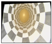 |  |  |
| Undisposed contour |  |  |  |  |
| Processed contour |  |  |  | 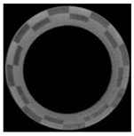 |
| Offset Condition | Undisposed Image | Processed Image |
|---|---|---|
| 0 mm |  |  |
| 5 mm |  |  |
| 10 mm |  |  |
| 15 mm |  |  |
| Offset Condition | Undisposed Image | Processed Image |
|---|---|---|
| 0° |  |  |
| 4° |  |  |
| 6° |  |  |
| 8° |  |  |
| Offset Condition | Undisposed Image | Processed Image |
|---|---|---|
| 0 mm and 0° |  |  |
| 5 mm and 8° |  |  |
| 10 mm and 8° | 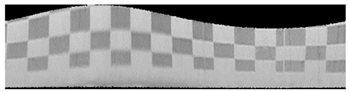 |  |
| 15 mm and 8° | 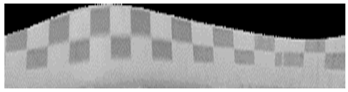 |  |
| Offset | Center Coordinates of the Circle before Correction | Center Coordinates of the Circle after Correction | Correction Rate | ||
|---|---|---|---|---|---|
| Inner Circle | Outer Circle | Inner Circle | Outer Circle | ||
| 5 mm | (351.0,598.0) | (351.0,592.5) | (350.6,598.0) | (350.2,597.9) | 92.5 |
| 10 mm | (363.5,593.5) | (357.8,589.5) | (364.0,594.2) | (363.9,593.6) | 91.4 |
| 15 mm | (340.0,595.0) | (331.0,591.5) | (341.1,595.9) | (340.3,595.1) | 91.8 |
| 4° | (427.5,602.5) | (451.8,601.5) | (424.2,602.6) | (427.2,602.5) | 87.7 |
| 6° | (246.5,627.5) | (224.0,626.5) | (250.7,627.8) | (247.3,627.5) | 84.9 |
| 8° | (298.0,599.0) | (325.9,599.5) | (292.5,598.8) | (297.5,598.8) | 82.1 |
| 5 mm-8° | (370.0,578.0) | (359.4,575.5) | (372.7,579.1) | (371.0,578.6) | 83.5 |
| 10 mm-8° | (376.0,596.0) | (361.8,593.5) | (379.2,596.8) | (376.4,595.5) | 78.5 |
| 15 mm-8° | (355.0,586.0) | (345.0,586.5) | (358.4,585.7) | (355.7,586.2) | 73.0 |
| Average deviation correction rate | 84.5 | ||||
| Radius Number | 1 | 2 | 3 | 4 | 5 | 6 | 7 |
|---|---|---|---|---|---|---|---|
| Average radius | 114.14 | 137.67 | 149.05 | 164.79 | 185.15 | 210.57 | 241.46 |
| Standard deviation | 0.41 | 0.48 | 0.36 | 0.45 | 0.36 | 0.43 | 0.43 |
| Average relative error | 0% | 0% | 0% | 0% | 0% | 0% | 0% |
| Offset Situation | 5 mm | 10 mm | 15 mm | ||||||
|---|---|---|---|---|---|---|---|---|---|
| Radius number | 5 | 6 | 7 | 5 | 6 | 7 | 5 | 6 | 7 |
| Average radius | 185.56 | 210.34 | 241.89 | 185.56 | 209.55 | 242.11 | 184.70 | 208.10 | 242.70 |
| Standard deviation | 0.52 | 0.30 | 0.73 | 0.52 | 1.03 | 0.77 | 0.60 | 2.50 | 1.31 |
| Average relative error | 0.25% | 0.11% | 0.23% | 0.25% | 0.47% | 0.27% | 0.24% | 1.17% | 0.51% |
| Offset Situation | 4 | 6 | 8 | ||||||
|---|---|---|---|---|---|---|---|---|---|
| Radius number | 3 | 4 | 5 | 3 | 4 | 5 | 3 | 4 | 5 |
| Average radius | 144.40 | 171.93 | 175.98 | 141.76 | 154.85 | 172.14 | 160.50 | 178.61 | 201.63 |
| Standard deviation | 4.66 | 7.20 | 9.18 | 7.75 | 10.14 | 13.12 | 9.88 | 13.84 | 16.50 |
| Average relative error | 3.12% | 4.20% | 4.95% | 4.90% | 6.03% | 7.02% | 6.20% | 7.78% | 8.23% |
| Offset Situation | Displacement and Angle | ||||||||
|---|---|---|---|---|---|---|---|---|---|
| 5 mm and 8° | 10 mm and 8° | 15 mm and 8° | |||||||
| Radius number | 1 | 2 | 3 | 1 | 2 | 3 | 1 | 2 | 3 |
| Average radius | 114.14 | 146.12 | 159.38 | 124.77 | 151.12 | 165.041 | 128.61 | 156.66 | 168.87 |
| Standard deviation | 6.53 | 8.46 | 10.34 | 10.73 | 13.46 | 16.04 | 14.48 | 18.01 | 19.84 |
Disclaimer/Publisher’s Note: The statements, opinions and data contained in all publications are solely those of the individual author(s) and contributor(s) and not of MDPI and/or the editor(s). MDPI and/or the editor(s) disclaim responsibility for any injury to people or property resulting from any ideas, methods, instructions or products referred to in the content. |
© 2024 by the authors. Licensee MDPI, Basel, Switzerland. This article is an open access article distributed under the terms and conditions of the Creative Commons Attribution (CC BY) license (https://creativecommons.org/licenses/by/4.0/).
Share and Cite
Zhang, Z.; Zhou, J.; Li, X.; Xu, C.; Hu, X.; Wang, L. Correction Method for Perspective Distortions of Pipeline Images. Electronics 2024, 13, 2898. https://doi.org/10.3390/electronics13152898
Zhang Z, Zhou J, Li X, Xu C, Hu X, Wang L. Correction Method for Perspective Distortions of Pipeline Images. Electronics. 2024; 13(15):2898. https://doi.org/10.3390/electronics13152898
Chicago/Turabian StyleZhang, Zheng, Jiazheng Zhou, Xiuhong Li, Chaobin Xu, Xinyu Hu, and Linhuang Wang. 2024. "Correction Method for Perspective Distortions of Pipeline Images" Electronics 13, no. 15: 2898. https://doi.org/10.3390/electronics13152898